Capacity of a Multiple-Antenna Fading Channel With a Quantized Precoding Matrix

Abstract

Given a multiple-input multiple-output (MIMO) channel, feedback from the receiver can be used to specify a transmit precoding matrix, which selectively activates the strongest channel modes. Here we analyze the performance of Random Vector Quantization (RVQ), in which the precoding matrix is selected from a random codebook containing independent, isotropically distributed entries. We assume that channel elements are i.i.d. and known to the receiver, which relays the optimal (rate-maximizing) precoder codebook index to the transmitter using $B$ bits. We first derive the large system capacity of beamforming (rank-one precoding matrix) as a function of $B$, where large system refers to the limit as $B$ and the number of transmit and receive antennas all go to infinity with fixed ratios. RVQ for beamforming is asymptotically optimal, i.e., no other quantization scheme can achieve a larger asymptotic rate. We subsequently consider a precoding matrix with arbitrary rank, and approximate the asymptotic RVQ performance with optimal and linear receivers (matched filter and Minimum Mean Squared Error (MMSE)). Numerical examples show that these approximations accurately predict the performance of finite-size systems of interest. Given a target spectral efficiency, numerical examples show that the amount of feedback required by the linear MMSE receiver is only slightly more than that required by the optimal receiver, whereas the matched filter can require significantly more feedback.

I Introduction

Given a multi-input multi-output (MIMO) channel, providing channel information at the transmitter can increase the achievable rate and simplify the coder and decoder. Namely, this channel information can specify a precoding matrix, which aligns the transmitted signal along the strongest channel modes (i.e., singular vectors corresponding to the largest singular values). In practice, the precoding matrix must be quantized at the receiver, and relayed to the transmitter via a feedback channel. The corresponding achievable rate is therefore limited by the accuracy of the quantizer.

The design and performance of quantized precoding matrices for multi-input single-output (MISO) and MIMO channels has been considered in numerous references, including [1, 2, 3, 4, 5, 6, 7, 8, 9, 10, 11, 12]. In those references, and in this paper, the channel is assumed to be stationary, known at the receiver, and the performance is evaluated as a function of the number of quantization bits $B$. (This is in contrast with other work, which models estimation error at the receiver, but does not explicitly account for quantization error (e.g., [13, 14]), and which assumes a time-varying channel with feedback of second-order statistics [15, 16, 17, 18].) Optimization of vector quantization codebooks is discussed in [1, 3, 2, 5, 6] for beamforming, and in [4, 12, 7] for MIMO channels with precoding matrices that provide multiplexing gain (i.e., have rank larger than one). It is shown in [3, 2] that this optimization can be interpreted as maximizing the minimum distance between points in a Grassmannian space. (See also [9].) The performance of this class of Grassmannian codebooks is also studied in [10, 8, 9].

In this paper, we evaluate the performance of a Random Vector Quantization (RVQ) scheme for the precoding matrix. Namely, given $B$ feedback bits, the precoding matrix is selected from a random codebook containing $2^{B}$ matrices, which are independent and isotropically distributed. RVQ has been analyzed in other source coding contexts (e.g., see [19] and the related discussion in [20]), and achieves the rate-distortion bound for ergodic Gaussian sources. This work is motivated by prior work [21] in which RVQ is considered for signature quantization in Code-Division Multiple Access (CDMA). In that scenario, limited feedback is used to select a signature for a particular user, which maximizes the received Signal-to-Interference-Plus-Noise-Ratio (SINR). RVQ has the attractive properties of being tractable and asymptotically optimal. Namely, in [21] the received SINR with RVQ is evaluated in the asymptotic (large system) limit as processing gain, number of users, and feedback bits all tend to infinity with fixed ratios. Furthermore, it is shown that no other quantization scheme can achieve a larger asymptotic SINR.

Here we assume an i.i.d. block Rayleigh fading channel model with independent channel gains, and take ergodic capacity as the performance criterion. The receiver relays $B$ bits to the transmitter (per codeword) via a reliable feedback channel (i.e., no feedback errors) with no delay. We start by evaluating the capacity of MISO and MIMO channels with a quantized beamformer, i.e., rank-one precoding matrix. Our results are asymptotic as the number of transmit antennas $N_{t}$ and feedback bits $B$ both tend to infinity with fixed $B/N_{t}$ (feedback bits per degree of freedom). For the MIMO channel the number of receive antennas $N_{r}$ also tends to infinity in proportion with $N_{t}$ and $B$. The asymptotic expressions accurately predict the performance of finite-size systems of interest as a function of normalized feedback and background Signal-to-Noise Ratio (SNR). In analogy with the optimality result shown in [21], RVQ is also asymptotically optimal in this scenario, i.e., no other quantization scheme can achieve a larger asymptotic rate. Furthermore, numerical examples for small $N_{t}$ show that RVQ performance averaged over codebooks is essentially the same as that obtained from codebooks optimized via the Lloyd-Max algorithm [1, 5, 6]. (See also the numerical examples in [22], which compare RVQ performance with the optimized (Grassmannian) codebooks in [3].)

We then consider quantization of a precoding matrix with arbitrary rank. Namely, a rank $K$ precoding matrix multiplexes $K$ independent streams of transmitted information symbols onto the $N_{t}$ transmit antennas. In that case, the capacity with limited feedback is approximated in the limit as $B$, $N_{t}$, $N_{r}$, and $K$ all tend to infinity with fixed ratios $K/N_{t}$, $N_{r}/N_{t}$, and $B/N_{r}^{2}$. That is, the number of feedback bits again scales linearly with the number of degrees of freedom, which is proportional to $N_{r}^{2}$. Although our results for beamforming suggest that RVQ is also asymptotically optimal in this scenario, this remains an open question.

The asymptotic results for a precoder matrix with arbitrary rank $K$ can be used to determine the normalized rank, or multiplexing gain $K/N_{t}$, which maximizes the capacity. This optimized rank in general depends on the normalized feedback, the ratio of antennas $N_{t}/N_{r}$, and the SNR. For example, if $N_{t}/N_{r}\geq 1$ and the SNR is sufficiently large, then as the feedback increases from zero to infinity, the optimized rank decreases from one to $N_{r}/N_{t}$. Numerical results are presented, which illustrate the effect of normalized rank on achievable rate, and also show that the asymptotic results accurately predict simulated results for finite-size systems of interest.

We also evaluate the performance of RVQ with linear receivers (i.e., the matched filter and linear Minimum Mean Squared Error (MMSE) receivers), and compare their performance with the optimal (capacity-achieving) receiver. With the optimal precoding matrix, corresponding to infinite feedback, both linear receivers are optimal. With limited feedback the two linear receivers are simpler than the optimal receiver, but require more feedback to achieve a target rate. Numerical results show that this additional feedback required by the linear MMSE receiver is quite small, whereas the additional feedback required by the matched filter can be significant (e.g., about one bit per precoding matrix element).

In addition to quantizing the optimal precoding matrix, power for each data stream can also be optimized, quantized, and fed back to the transmitter (e.g., see [23, 24]). Asymptotically, the amount of feedback required to specify the power is negligible compared to the feedback required for the precoding matrix. Furthermore, uniform power over the set of activated channel typically performs close to the optimal (water-filling) performance [8]. We therefore only consider quantization of the precoding matrix.

Other related work on RVQ for MIMO channels has been presented in [25, 26, 27]. Namely, exact expressions for the ergodic capacity with beamforming and RVQ for a finite-size MISO channel are derived in [25]. The performance of RVQ for precoding over a broadcast MIMO channel is analyzed in [26, 27]. A closely related random beamforming scheme for the multiuser MIMO broadcast channel was previously presented in [28]. In that work, the growth in sum capacity is characterized asymptotically as the number of users becomes large with a fixed number of antennas. (Random beamforming was previously proposed in [29], although there the main focus is to improve fairness among users.)

The paper is organized as follows. Section II describes the channel model, Section III considers the capacity of beamforming with limited feedback, and sections IV and V examine the capacity of a quantized precoding matrix with optimal and linear receivers, respectively. Derivations of the main results are given in the appendices.

II Channel Model

We consider a point-to-point, flat Rayleigh fading channel with $N_{t}$ transmit antennas and $N_{r}$ receive antennas. Let $\bm{x}=[x_{k}]$ be a $K\times 1$ vector of transmitted symbols with covariance matrix $\bm{I}_{K}$, where $\bm{I}_{K}$ is the $K\times K$ identity matrix, and $K$ is the number of independent data streams. The received $N_{r}\times 1$ vector is given by

$$\bm{y}=\frac{1}{\sqrt{K}}\bm{H}\bm{V}\bm{x}+\bm{n}$$ (1)

where $\bm{H}=[h_{n_{r},n_{t}}]$ is an $N_{r}\times N_{t}$ channel matrix, $\bm{V}=[\bm{v}_{1}\ \bm{v}_{2}\ \ldots\ \bm{v}_{K}]$ is an $N_{t}\times K$ precoding matrix, and $\bm{n}$ is a complex Gaussian noise $N_{r}\times 1$ vector with covariance matrix $\sigma_{n}^{2}\bm{I}_{N_{r}}$. Assuming rich scattering and Rayleigh fading, the elements of $\bm{H}$ are independent, and the channel coefficient between the $n_{t}$th transmit antenna and the $n_{r}$th receive antenna, $h_{n_{r},n_{t}}$, is a circularly symmetric complex Gaussian random variable with zero mean and unit variance ($E[|h_{n_{r},n_{t}}|^{2}]=1$).

We assume i.i.d. block fading, i.e., the channel is static within a fading block, and the channels across blocks are independent. The ergodic capacity is achieved by coding the transmitted symbols across an infinitely large number of fading blocks. With perfect channel knowledge at the receiver and a given precoding matrix $\bm{V}$, the ergodic capacity is the mutual information between $\bm{x}$ and $\bm{y}$ with a complex Gaussian distributed input, averaged over the channel, given by

$$I(\bm{x};\bm{y})=E_{\bm{H}}\left[\log\det\left(\bm{I}+\frac{\rho}{K}\bm{H}\bm{V}\bm{V}^{{\dagger}}\bm{H}^{{\dagger}}\right)\right]$$ (2)

where $\rho=1/\sigma_{n}^{2}$ is the background SNR. We wish to specify the precoding matrix $\bm{V}$ that maximizes the mutual information, subject to a power constraint $\|\bm{v}_{k}\|\leq 1$, for $1\leq k\leq K$.

With unlimited feedback, the columns of the optimal precoding matrix, which maximizes (2), are eigenvectors of the channel covariance matrix $\bm{H}^{{\dagger}}\bm{H}$. With $B$ feedback bits per fading block, we can specify the precoding matrix from a quantization set or codebook $\mathcal{V}=\{\bm{V}_{1},\cdots,\bm{V}_{2^{B}}\}$ known a priori to both the transmitter and receiver. The receiver chooses the $\bm{V}_{j}$ that maximizes the sum mutual information, and relays the corresponding index back to the transmitter. Of course, the performance (ergodic capacity) depends on the codebook $\mathcal{V}$.

III Beamforming with Limited Feedback

We start with a rank-one precoding matrix, corresponding to a single data stream ($K=1$). In that case, the precoding matrix is specified by an $N_{t}\times 1$ beamforming vector $\bm{v}$, which ideally corresponds to the strongest channel mode. That is, the optimal $\bm{v}$, which maximizes the ergodic capacity in (2), is the eigenvector of $\bm{H}^{\dagger}\bm{H}$ corresponding to the largest eigenvalue. This vector is computed at the receiver and a quantized version is relayed back to the transmitter.

Let $\mathcal{V}=\{\bm{v}_{1},\ldots,\bm{v}_{2^{B}}\}$ denote the quantization codebook for $\bm{v}$, given $B$ feedback bits. Optimization of this codebook has been considered in [3, 2, 6] with outage capacity and ergodic capacity as performance metrics. The performance of an optimized codebook is difficult to evaluate exactly, and is approximated in [3, 2, 6, 10, 9, 11]. Here we consider RVQ in which $\bm{v}_{1},\cdots,\bm{v}_{2^{B}}$ are independent, isotropically distributed random vectors, each with unit norm. This is motivated by the observation that given a channel matrix $\bm{H}$ with i.i.d. elements, the eigenvectors of $\bm{H}^{\dagger}\bm{H}$ are isotropically distributed [30], hence the codebook entries should be uniformly distributed over the space of beamforming vectors.

III-A MISO Channel

We first consider a MISO channel, corresponding to a single receive antenna ($N_{r}=1$). In that case, $\bm{H}$ is an $N_{t}\times 1$ channel vector, which we denote as $\bm{h}$. The optimal beamformer, which maximizes the mutual information in (2), is the normalized channel vector $\bm{h}/\|\bm{h}\|$ and the corresponding mutual information is $E_{\bm{h}}[\log(1+\rho\bm{h}^{{\dagger}}\bm{h})]$. The receiver selects the quantized precoding vector to maximize the mutual information, i.e.,

$$\hat{\bm{v}}=\arg\max_{1\leq j\leq 2^{B}}\left\{I_{j}=\log(1+\rho|\bm{h}^{{\dagger}}\bm{v}_{j}|^{2})\right\}$$ (3)

and the corresponding achievable rate is

$$I_{\textsf{rvq}}^{N_{t}}\triangleq\max_{1\leq j\leq 2^{B}}I_{j}.$$ (4)

where the superscript $N_{t}$ denotes the system size. The achievable rate depends on the codebook $\mathcal{V}$ and the channel vector $\bm{h}$, and is therefore random. Rather than averaging $I_{\textsf{rvq}}^{N_{t}}$ over $\mathcal{V}$ and $\bm{h}$ to find the ergodic capacity, we instead evaluate the limiting performance as $N_{t}$ and $B$ tend to infinity with fixed $\bar{B}=B/N_{t}$ (feedback bits per transmit antenna). In this limit, $I_{\textsf{rvq}}^{N_{t}}$ converges to a deterministic constant. This is illustrated in Fig. 1, which shows the pdf of $|\bm{h}^{\dagger}\hat{\bm{v}}|^{2}/\|\bm{h}\|^{2}$ for different $N_{t}$ with no feedback ($\bar{B}=0$), and for RVQ with $\bar{B}=2$. The figure shows that convergence of the pdf to a point mass is faster with feedback than without.

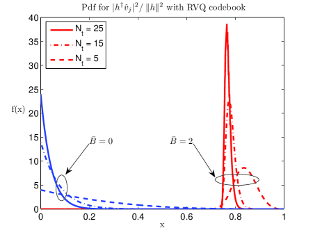
Figure 1: pdf of $|\bm{h}^{\dagger}\hat{\bm{v}}|^{2}/\|\bm{h}\|^{2}$ with RVQ for different values of $N_{t}$.

As $N_{t}\to\infty$, $(\bm{h}^{\dagger}\bm{h})/N_{t}\to 1$ almost surely, so that $\log(1+\rho\bm{h}^{\dagger}\bm{h})-\log(\rho N_{t})\to 0$. That is, with perfect channel knowledge at the transmitter, the ergodic capacity increases as $\log(\rho N_{t})$. With finite feedback there is a rate loss, which is defined as

$$I_{\textsf{rvq}}^{\triangle}=I_{\textsf{rvq}}^{N_{t}}-\log(\rho N_{t}).$$ (5)

For finite $N_{t}$, $I_{\textsf{rvq}}^{\triangle}$ is random; however, in the large system limit $I_{\textsf{rvq}}^{\triangle}$ converges to a deterministic constant.

Theorem 1.

As $(N_{t},B)\to\infty$ with fixed $\bar{B}=B/N_{t}$, the rate difference $I_{\textsf{rvq}}^{\triangle}$ converges in the mean square sense to

$$\mathcal{I}_{\textsf{rvq}}^{\triangle}=\log(1-2^{-\bar{B}}).$$ (6)

The proof is given in Appendix -A. For $\bar{B}>0$, the rate loss due to finite feedback is a constant. As $\bar{B}\to 0$, this rate loss tends to infinity, since with $\bar{B}=0$, the capacity tends to a constant as $N_{t}\to\infty$, whereas the capacity grows as $\log N_{t}$ for $\bar{B}>0$. Of course, as $\bar{B}\to\infty$ (unlimited feedback), the rate loss vanishes.

RVQ is asymptotically optimal in the following sense. Suppose that $\{\mathcal{V}_{N_{t}}\}$ is an arbitrary sequence of codebooks for the beamforming vector where

$$\mathcal{V}_{N_{t}}=\left\{\bm{v}_{1}^{N_{t}},\bm{v}_{2}^{N_{t}},\ldots,\bm{v}_{2^{B}}^{N_{t}}\right\}$$ (7)

is the codebook for a particular $N_{t}$ and $\|\bm{v}_{j}^{N_{t}}\|^{2}=1$ for each $j$. The associated rate is given by

$$I_{\mathcal{V}_{N_{t}}}=\max_{1\leq j\leq 2^{B}}\log(1+\rho|\bm{h}^{{\dagger}}\bm{v}_{j}^{N_{t}}|^{2})$$ (8)

and the rate difference $I^{\triangle}_{\mathcal{V}_{N_{t}}}=I_{\mathcal{V}_{N_{t}}}-\log(\rho N_{t})$.

Theorem 2.

For any sequence of codebooks $\{\mathcal{V}_{N_{t}}\}$,

$$\limsup_{(N_{t},B)\to\infty}E_{\bm{h}}[I^{\triangle}_{\mathcal{V}_{N_{t}}}]\leq\mathcal{I}_{\textsf{rvq}}^{\triangle}.$$ (9)

The proof is given in Appendix -B.

Although the optimality of RVQ holds only in the large system limit, numerical results in Section III-C show that for finite-size systems of interest RVQ performs essentially the same as optimized quantization codebooks.

III-B Multi-Input Multi-Output (MIMO) Channel

We now consider quantized beamforming for a MIMO channel, i.e., with multiple transmit and receive antennas. Taking the rank $K=1$ maximizes the diversity gain [31], but the corresponding capacity grows only as $\log N_{t}$ instead of linearly with $N_{t}$, which is the case when $K$ grows proportionally with $N_{t}$. (This is true with both unlimited and limited feedback, assuming a fixed number of feedback bits per precoder element.) Also, a beamformer is significantly less complex than a matrix precoder with $K>1$, and requires less feedback to specify.

We again consider an RVQ codebook $\mathcal{V}$ with $2^{B}$ independent unit-norm vectors, where each vector is uniformly distributed over the $N_{t}$-dimensional unit sphere. The achievable rate is $E_{\bm{H}}[I_{\textsf{rvq}}^{N_{t}}]$, where

$$I_{\textsf{rvq}}^{N_{t}} = E_{\mathcal{V}}\left[\left.\max_{1\leq j\leq 2^{B}}\log\left(1+\rho\|\bm{H}\bm{v}_{j}\|^{2}\right)\right|\bm{H}\right]$$ (10)

$$= E_{\mathcal{V}}\left[\log(1+\rho\left.\max_{1\leq j\leq 2^{B}}\|\bm{H}\bm{v}_{j}\|^{2})\right|\bm{H}\right].$$ (11)

As for the MISO channel, with unlimited feedback the achievable rate increases as $\log(\rho N_{t})$. We again define the rate difference due to quantization as

$$I^{\triangle}_{\textsf{rvq}}\triangleq I_{\textsf{rvq}}^{N_{t}}-\log(\rho N_{t})=E_{\mathcal{V}}\left[\left.\log\left(\frac{1}{\rho N_{t}}+\max_{j}\gamma_{j}\right)\right|\bm{H}\right]$$ (12)

where

$$\gamma_{j}=\frac{1}{N_{t}}\bm{v}_{j}^{\dagger}\bm{H}^{\dagger}\bm{H}\bm{v}_{j}.$$ (13)

Evaluating the expectation in (12) is difficult for finite $N_{t}$, $N_{r}$, and $B$, so that we again resort to a large system analysis. Namely, we let $N_{t}$, $N_{r}$, and $B$ each tend to infinity with fixed $\bar{B}=B/N_{t}$ and $\bar{N}_{r}=N_{r}/N_{t}$. For each $N_{t}$ and $N_{r}$ the channel matrix $\bm{H}$ is chosen as the $N_{r}\times N_{t}$ upper-left corner of a matrix $\bar{\bm{H}}$ with an infinite number of rows and columns, and with i.i.d. complex Gaussian entries.

The received power in this large system limit is given by

$$\gamma^{\infty}_{\textsf{rvq}}=\lim_{(N_{t},N_{r},B)\to\infty}\left[\left.\max_{1\leq j\leq 2^{B}}\gamma_{j}\right|\bar{\bm{H}}\right]$$ (14)

where convergence to the deterministic limit can be shown in the mean square sense. Conditioned on $\bar{\bm{H}}$, the $\gamma_{j}$’s are i.i.d. since the beamforming vectors $\bm{v}_{j}$ are i.i.d., and applying [32, Theorem 2.1.2], it can be shown that

$$\gamma^{\infty}_{\textsf{rvq}}=\lim_{(N_{t},N_{r},B)\to\infty}F^{-1}_{\gamma|\bar{\bm{H}}}\left(1-2^{-B}\right)$$ (15)

where $F_{\gamma|\bar{\bm{H}}}(\cdot)$ is the cdf of $\gamma_{j}$ given $\bar{\bm{H}}$. Analogous results for the interference power in CDMA with quantized signatures have been presented in [21], so that we omit the proofs of (14) and (15). Note that $\bar{N}_{r}\leq\gamma^{\infty}_{\textsf{rvq}}\leq(1+\sqrt{\bar{N}_{r}})^{2}$, where the lower and upper bounds correspond to $\bar{B}=0$ and $\bar{B}=\infty$, respectively. That is, $(1+\sqrt{\bar{N}_{r}})^{2}$ is the asymptotic maximum eigenvalue of the channel covariance matrix $\frac{1}{N_{t}}\bm{H}^{{\dagger}}\bm{H}$ [33]. The asymptotic rate difference is given by

$$\mathcal{I}_{\textsf{rvq}}^{\Delta}=\lim_{(N_{t},N_{r},B)\to\infty}I^{\Delta}_{\textsf{rvq}}=\log(\gamma^{\infty}_{\textsf{rvq}})$$ (16)

The limit in (15) can be explicitly evaluated, and is independent of the channel realization $\bar{\bm{H}}$.

Theorem 3.

For $0\leq\bar{B}\leq\bar{B}^{*}$, $\gamma_{\textsf{rvq}}^{\infty}$ satisfies

$$\left(\gamma_{\textsf{rvq}}^{\infty}\right)^{\bar{N}_{r}}\mathrm{e}^{-\gamma_{\textsf{rvq}}^{\infty}}=2^{-\bar{B}}\left(\frac{\bar{N}_{r}}{\mathrm{e}}\right)^{\bar{N}_{r}}$$ (17)

and for $\bar{B}\geq\bar{B}^{*}$,

$$\begin{split}\gamma_{\textsf{rvq}}^{\infty}&=(1+\sqrt{\bar{N}_{r}})^{2}-\exp\big{\{}\frac{1}{2}\bar{N}_{r}\log(\bar{N}_{r})\\ &\quad-(\bar{N}_{r}-1)\log(1+\sqrt{\bar{N}_{r}})+\sqrt{\bar{N}_{r}}-\bar{B}\log(2)\big{\}}\end{split}$$ (18)

where

$$\bar{B}^{*}=\frac{1}{\log(2)}\left(\bar{N}_{r}\log\left(\frac{\sqrt{\bar{N}_{r}}}{1+\sqrt{\bar{N}_{r}}}\right)+\sqrt{\bar{N}_{r}}\right).$$ (19)

The proof is given in Appendix -C and is motivated by an analogous result for CDMA, presented in [34]. As stated in Theorem 3, $\gamma_{\textsf{rvq}}^{\infty}$ depends only on $\bar{B}$ and $\bar{N}_{r}$. Letting $\bar{N}_{r}\to 0$ gives the the asymptotic capacity of the MISO channel with RVQ. As for the MISO channel, RVQ is asymptotically optimal.

Theorem 4.

As $(N_{t},N_{r},B)\to\infty$ with fixed $\bar{N}_{r}=N_{r}/N_{t}$ and $\bar{B}=B/N_{t}$,

$$\limsup_{(N_{t},N_{r},B)\to\infty}I_{\mathcal{V}_{N_{t}}}^{N_{t}}-\log(\rho N_{t})\leq\mathcal{I}_{\textsf{rvq}}^{\Delta}$$ (20)

for any sequence of codebooks $\{\mathcal{V}_{N_{t}}\}$.

The proof is similar to the proof of Theorem 2 in [21] and is therefore omitted.

III-C Numerical Results

Figs. 2 and 3 show $\mathcal{I}_{\textsf{rvq}}^{\triangle}$ for MISO and MIMO channels, respectively, with beamforming and RVQ versus normalized feedback bits ($\bar{B}$) with $\rho=5$ and 10 dB. Also shown for comparison are achievable rates with a quantization codebook optimized via the Lloyd-Max algorithm [1, 5, 6], and the capacity with perfect beamforming, corresponding to unlimited feedback. The results for RVQ are averaged over codebook realizations, and are essentially the same as those shown for the optimized Lloyd-Max codebooks. For the MISO channel, the asymptotic capacity (6) accurately predicts the simulated results shown even with a relatively small number of transmit antennas ($N_{t}=3\text{ and }6$). For the MIMO results $\bar{N}_{r}=1.5$, and simulation results are shown for $4\times 6$ and $16\times 24$ channels. The asymptotic results accurately predict the performance for the larger channel, and are somewhat less accurate for the smaller channel.

Comparing finite feedback with perfect beamforming, the results show that one feedback bit per complex entry ($\bar{B}=1$) provides more than 50% of the potential gain due to feedback. For both the MISO and MIMO examples shown, the perfect beamforming capacity is nearly achieved with two feedback bits per complex coefficient.

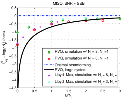
Figure 2: Asymptotic and simulated rate differences versus feedback bits for a MISO channel with beamforming.

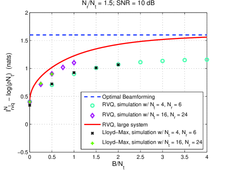
Figure 3: Asymptotic and simulated rate differences versus feedback bits for a MIMO channel with beamforming ($\bar{N}_{r}=1.5$).

IV Precoding Matrix with Arbitrary Rank

In this section we consider the performance of a single-user MIMO channel with precoding matrix $\bm{V}$ having rank $K>1$. We wish to determine the asymptotic capacity with RVQ as in the previous section. Here we consider the large system limit as $(N_{t},N_{r},B,K)\to\infty$ with fixed ratios $\bar{N}_{r}=N_{r}/N_{t}$, $\hat{B}=B/N_{r}^{2}$, and $\bar{K}=K/N_{t}$. That is, we scale the rank of the precoding matrix with $N_{t}$. The number of feedback bits is normalized by $N_{r}^{2}$, instead of $N_{r}$, since the feedback must scale linearly with degrees of freedom (in this case the number of channel elements $N_{r}N_{t}$).) Given a fixed number of feedback bits per channel coefficient, the capacity grows linearly with the number of antennas ($N_{t}$ or $N_{r}$).

Given a rank $K\leq N_{t}$, the precoding matrix is chosen from the RVQ set

$$\mathcal{V}=\{\bm{V}_{j},1\leq j\leq 2^{B}\},$$ (21)

where the entries are independent $N_{t}\times K$ random unitary matrices, i.e., $\bm{V}_{j}^{{\dagger}}\bm{V}_{j}=\bm{I}_{K}$. This codebook is an extension of the RVQ codebook for beamforming. Letting

$$J^{N_{r}}_{j}=\frac{1}{N_{r}}\log\det\left(\bm{I}_{N_{r}}+\frac{\rho}{K}\bm{H}\bm{V}_{j}\bm{V}_{j}^{{\dagger}}\bm{H}^{{\dagger}}\right),$$ (22)

the receiver again selects the quantized precoding matrix, which maximizes the mutual information

$$\hat{\bm{V}}=\arg\max_{\quad 1\leq j\leq 2^{B}}J^{N_{r}}_{j}.$$ (23)

For finite $N_{r}$, we define

$$I_{\textsf{rvq}}^{N_{r}} =E_{\mathcal{V}}[\max_{\quad 1\leq j\leq 2^{B}}J^{N_{r}}_{j}|\bar{\bm{H}}]$$ (24)

$$=E_{\mathcal{V}}\left[\left.\frac{1}{N_{r}}\log\det\left(\bm{I}_{N_{r}}+\frac{\rho}{K}\bm{H}\hat{\bm{V}}\hat{\bm{V}}^{{\dagger}}\bm{H}^{{\dagger}}\right)\right|\bar{\bm{H}}\right]$$ (25)

and the average sum mutual information per receive antenna with $B$ feedback bits is then $E_{\bm{H}}[I_{\textsf{rvq}}^{N_{r}}]$.

Here the power allocation over channel modes is “on-off”. Namely, active modes are assigned equal powers. This simplifies the analysis, and it has been observed that the additional gain due to an optimal power allocation (water pouring) is quite small [8].

Since the entries of the RVQ codebook are i.i.d., the mutual informations $J^{N_{r}}_{j},j=1,\ldots,2^{B}$, are also i.i.d. for a given $\bm{H}$. In principle, the large system limit of $I_{\textsf{rvq}}^{N_{r}}$ can be evaluated, in analogy with (15), given the cdf of $J^{N_{r}}_{j}$ given $\bm{H}$, denoted as $F_{J;N_{r}|\bm{H}}$. This cdf appears to be difficult to determine in closed-form for general $(N_{r},N_{t},K)$, so that we are unable to derive the exact asymptotic capacity with RVQ. Still, we can provide an accurate approximation for this large system limit. Before presenting this approximation, we first compare the capacity with no channel information at the transmitter ($\hat{B}=0$) to the capacity with perfect channel information ($\hat{B}=\infty$).

If $\hat{B}=0$, then the optimal transmit covariance matrix $\bm{V}\bm{V}^{{\dagger}}=\bm{I}_{N_{t}}$ and $K=N_{t}$ [35]. That is, all channel modes are allocated equal power. As $(N_{t},N_{r})\to\infty$ with fixed $\bar{N}_{r}=N_{r}/N_{t}$, the capacity per receive antenna is given by

$$\frac{1}{N_{r}}\log\det\left(\bm{I}_{N_{r}}+\frac{\rho}{N_{t}}\bm{H}\bm{H}^{{\dagger}}\right) \to\int_{0}^{\infty}\log\left(1+\rho\lambda\right)g(\lambda)\,\mathrm{d}\lambda$$ (26)

$$=\mathcal{I}_{\textsf{rvq}}(\hat{B}=0)$$ (27)

where convergence is in the almost sure sense, and $g(\lambda)$ is the asymptotic probability density function for a randomly chosen eigenvalue of $\frac{1}{N_{t}}\bm{H}\bm{H}^{{\dagger}}$, and is given by [33]

$$g(\lambda)=\frac{\sqrt{(\lambda-a)(b-\lambda)}}{2\pi\lambda\bar{N}_{r}}\quad{\mathrm{for}}\quad a\leq\lambda\leq b,$$ (28)

$$a=\left(1-\sqrt{\bar{N}_{r}}\right)^{2}\quad{\mathrm{and}}\quad b=\left(1+\sqrt{\bar{N}_{r}}\right)^{2}$$ (29)

for $\bar{N}_{r}\leq 1$. The integral in (26) has been evaluated in [36], which gives the closed-form expression

$$\mathcal{I}_{\textsf{rvq}}(\hat{B}=0)=\log\rho y+\frac{1-\bar{N}_{r}}{\bar{N}_{r}}\log\left(\frac{1}{1-z}\right)-\frac{z}{\bar{N}_{r}}$$ (30)

where

$$y =\frac{1}{2}\left(1+\bar{N}_{r}+\frac{1}{\rho}+\sqrt{\left(1+\bar{N}_{r}+\frac{1}{\rho}\right)^{2}-4\bar{N}_{r}}\right)$$ (31)

$$z =\frac{1}{2}\left(1+\bar{N}_{r}+\frac{1}{\rho}-\sqrt{\left(1+\bar{N}_{r}+\frac{1}{\rho}\right)^{2}-4\bar{N}_{r}}\right).$$ (32)

If $\hat{B}=\infty$, then the $K$ columns of the optimal $\bm{V}$ are the eigenvectors of the channel covariance matrix corresponding to the $K$ largest eigenvalues. As $(N_{t},N_{r},B)\to\infty$, we have

$$\mathcal{I}_{\textsf{rvq}}(\hat{B}=\infty)=\int_{\eta}^{\infty}\log\left(1+\frac{\rho}{\bar{K}}\lambda\right)g(\lambda)\,\mathrm{d}\lambda$$ (33)

where $\eta$ satisfies

$$\int_{\eta}^{\infty}g(\lambda)\,\mathrm{d}\lambda=\min\{1,\frac{\bar{K}}{\bar{N}_{r}}\}$$ (34)

for $\bar{N}_{r}\leq 1$. We emphasize that this corresponds to a uniform allocation of power over the set of $K$ active eigenvectors. (This result has also been presented in [8].) The rank of the optimal $\bm{V}$, or optimal multiplexing gain, is at most $\min\{N_{t},N_{r}\}$ and can be obtained by differentiating (33) with respect to $\bar{K}$. It can be verified that $\mathcal{I}_{\textsf{rvq}}(\hat{B}=0)\leq\mathcal{I}_{\textsf{rvq}}(\hat{B}=\infty)$.

To illustrate the increase in capacity with feedback, in Fig. 4 we plot the rate ratio $\mathcal{I}_{\textsf{rvq}}(\hat{B}=\infty)/\mathcal{I}_{\textsf{rvq}}(\hat{B}=0)$ versus SNR for different values of $\bar{N}_{r}$, where $\mathcal{I}_{\textsf{rvq}}(\hat{B}=\infty)$ is optimized over rank $K$. For large SNR $\rho$, we can expand

$$\mathcal{I}_{\textsf{rvq}}(\hat{B}=0) =\log(\rho)+o(\log(\rho))$$ (35)

$$\mathcal{I}_{\textsf{rvq}}(\hat{B}=\infty) =\log(\rho)\int_{\eta}^{\infty}g(\lambda)\,\mathrm{d}\lambda+o(\log(\rho)).$$ (36)

Therefore

$$\lim_{\rho\to\infty}\frac{\mathcal{I}_{\textsf{rvq}}(\hat{B}=\infty)}{\mathcal{I}_{\textsf{rvq}}(\hat{B}=0)}=\int_{\eta}^{\infty}g(\lambda)\,\mathrm{d}\lambda\\ =\min\{1,\frac{\bar{K}}{\bar{N}_{r}}\}$$ (37)

which implies that the optimal rank $K^{*}=\min\{N_{t},N_{r}\}$, and the corresponding asymptotic rate ratio is one. The increase in achievable rate from feedback is small in this case, since for large SNRs, the transmitter excites all channel modes, and the uniform power allocation asymptotically gives the same capacity as water pouring. Of course, although the increase in rate is small, feedback can simplify coding and decoding.

For small $\rho$, we can expand $\log(1+\rho\lambda)$ and $\log(1+\rho\lambda/\bar{K})$ in Taylor series. Taking $\rho\to 0$ gives

$$\lim_{\rho\to 0} \frac{\mathcal{I}_{\textsf{rvq}}(\hat{B}=\infty)}{\mathcal{I}_{\textsf{rvq}}(\hat{B}=0)}$$

$$=\frac{1}{\bar{K}}\int_{\eta}^{\infty}\lambda g(\lambda)\,\mathrm{d}\lambda\leq\frac{1}{\bar{N}_{r}}\frac{\int_{\eta}^{\infty}\lambda g(\lambda)\,\mathrm{d}\lambda}{\int_{\eta}^{\infty}g(\lambda)\,\mathrm{d}\lambda}$$ (38)

$$\leq\frac{1}{\bar{N}_{r}}\frac{b\int_{\eta}^{b}g(\lambda)\,\mathrm{d}\lambda}{\int_{\eta}^{b}g(\lambda)\,\mathrm{d}\lambda}=\left(1+\frac{1}{\sqrt{\bar{N}_{r}}}\right)^{2}$$ (39)

where $b$ is the asymptotic maximum eigenvalue given by (29). The inequality in (38) follows from (34), which implies $\bar{K}\geq\bar{N}_{r}\int_{\eta}^{\infty}g(\lambda)\,\mathrm{d}\lambda$. Note that (39) corresponds to allocating all transmission power to the strongest channel mode, which is known to maximize capacity at low SNRs. The maximal rate ratio (39) can also be obtained from Theorem 3.

The rate increase due to feedback is substantial when $\bar{N}_{r}$ is small, and the rate ratio tends to infinity as $\bar{N}_{r}\to 0$. This is because the channel becomes a MISO channel, in which case the capacity is a constant with $\bar{B}=0$ and increases as $\log(\rho N_{t})$ with $\bar{B}=\infty$.

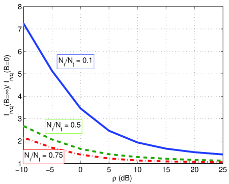
Figure 4: The rate ratio $\mathcal{I}_{\textsf{rvq}}(\hat{B}=\infty)/\mathcal{I}_{\textsf{rvq}}(\hat{B}=0)$ versus SNR (dB) for various values of $\bar{N}_{r}$.

To evaluate the asymptotic capacity with arbitrary $\hat{B}$, we approximate $J_{j}^{N_{r}}$ given $\bar{\bm{H}}$ as a Gaussian random variable. This is motivated by the fact that $J_{j}^{N_{r}}$ is Gaussian in the large system limit [37], since $\bm{H}\bm{V}$ is i.i.d. Conditioning on $\bm{H}$ introduces dependence among the elements of $\bm{H}\bm{V}$; however, numerical examples indicate that the Gaussian assumption is still valid for large $N_{t}$ and $N_{r}$. Alternatively, if we do not condition on $\bm{H}$, then the rates $\{J_{j}^{N_{r}}\}$ are dependent. Application of the results from extreme statistics, assuming the rates $\{J_{j}^{N_{r}}\}$ are independent, gives an upper bound on the asymptotic achievable rate (e.g., see the proof of Theorem 2 in [21]). This is illustrated by subsequent numerical results.

Evaluating the large system limit of $I_{\textsf{rvq}}^{N_{r}}$, assuming that the cdf of $J_{j}^{N_{r}}$ is Gaussian, gives the approximate rate

$$\tilde{\mathcal{I}}_{\textsf{rvq}}=\mu_{J}+\sigma_{J}\sqrt{2\hat{B}\log 2}$$ (40)

independent of the channel realization, where $\mu_{J}$ and $\sigma_{J}^{2}$ are the asymptotic mean of $J_{j}^{N_{r}}$, and variance of $N_{r}^{2}J_{j}^{N_{r}}$, respectively. The derivation of (40) is a straightforward extension of [32, Sec. 2.3.2] and is not shown here. As $\hat{B}\to 0$, this approximation becomes exact. However, as $\hat{B}\to\infty$, the approximate rate $\tilde{\mathcal{I}}_{\textsf{rvq}}\to\infty$, whereas the actual rate $\mathcal{I}_{\textsf{rvq}}(\hat{B}=\infty)$ is finite, and can be computed from (33) and (34). This is because $J_{j}^{N_{r}}$ is bounded for all $N_{r}$, whereas a Gaussian random variable can assume arbitrarily large values. Therefore the Gaussian approximation gives an inaccurate estimate of $\mathcal{I}_{\textsf{rvq}}$ for large $\hat{B}$. (This implies that we should approximate $\mathcal{I}_{\textsf{rvq}}$ as $\min\{\tilde{\mathcal{I}}_{\textsf{rvq}},\mathcal{I}_{\textsf{rvq}}(\hat{B}=\infty)\}$.)

The asymptotic mean and variance of $J_{j}^{N_{r}}$ are computed in Appendix -D. The asymptotic mean is given by

$$\begin{split}\mu_{J}=\frac{\bar{K}}{\bar{N}_{r}}\log\left(1+\frac{\bar{N}_{r}}{\bar{K}}\rho-\frac{\bar{N}_{r}}{\bar{K}}\rho v\right)\\ +\log\left(1+\rho-\frac{\bar{N}_{r}}{\bar{K}}\rho v\right)-v\end{split}$$ (41)

where

$$v=\frac{1}{2}+\frac{\bar{K}}{2\bar{N}_{r}}+\frac{\bar{K}}{2\bar{N}_{r}\rho}-\frac{1}{2}\sqrt{\left(1+\frac{\bar{K}}{\bar{N}_{r}}+\frac{\bar{K}}{\bar{N}_{r}\rho}\right)^{2}-\frac{4\bar{K}}{\bar{N}_{r}}}.$$ (42)

The asymptotic variance is approximated for $0\leq\bar{K}=\bar{N}_{r}\leq 1$ and small SNR ($\rho\leq-5\,\text{dB}$) as

$$\sigma_{J}^{2}\approx\rho^{2}(1-\bar{N}_{r}).$$ (43)

The asymptotic variance for moderate SNRs and normalized rank $\bar{K}\neq\bar{N}_{r}$ can be computed easily via numerical simulation.

In contrast with the beamforming results in the preceding section, we are unable to show that RVQ is asymptotically optimal when the precoding matrix has arbitrary rank. The corresponding argument for beamforming relies on the evaluation of the asymptotic rate difference $\mathcal{I}_{\textsf{rvq}}^{\Delta}$. Since here we are unable to evaluate $\mathcal{I}_{\textsf{rvq}}$ exactly, we cannot apply that argument. Nevertheless, numerical results have indicated that the performance of RVQ matches that of optimized codebooks (e.g., see [22]).

Fig. 5 shows $\tilde{\mathcal{I}}_{\textsf{rvq}}$ with normalized rank $\bar{K}=\bar{N}_{r}$ versus $\hat{B}$ for $\rho=-5,0,5\ \text{dB}$ and $\bar{N}_{r}=0.5$. The dashed lines show the unlimited feedback capacity $\mathcal{I}_{\textsf{rvq}}(\hat{B}=\infty)$, which is computed from (33) with optimized $\bar{K}$. The asymptotic rate with RVQ is computed from (40), where $\sigma_{J}$ for $\rho=-5\,\text{dB}$ is approximated by (43), and $\sigma_{J}$ is determined from simulation with $N_{t}=20$ for $\rho=0\text{ and }5\text{ dB}$. Also shown in Fig. 5 are simulation results for $\mathcal{I}_{\textsf{rvq}}$ with $N_{t}=8$ and $N_{r}=4$. Because the size of the RVQ codebook increases exponentially with $\hat{B}$, it is difficult to generate simulation results for moderate to large values of $\hat{B}$. Hence simulation results are shown only for $\hat{B}\leq 0.8$. The asymptotic results accurately approximate the simulated results shown. The accuracy increases as the feedback $\hat{B}$ decreases.

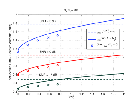
Figure 5: Sum mutual information per receive antenna with RVQ and an optimal receiver versus normalized feedback. The asymptotic approximation is shown along with Monte Carlo simulation results for an $8\times 4$ channel.

Since $\tilde{\mathcal{I}}_{\textsf{rvq}}$ is a function of both rank $\bar{K}$ and feedback $\hat{B}$, for a given $\hat{B}$, we can select $\bar{K}$ to maximize $\tilde{\mathcal{I}}_{\textsf{rvq}}$. Fig. 6 shows mutual information per receive antenna versus normalized rank from (40) with $\bar{N}_{r}=0.2$, $\rho=5$ dB, and different values of $\hat{B}$. ($\sigma_{J}$ is obtained from numerical simulations.) The maximal rates are attained at $\bar{K}=1$, $0.3$, and $0.2$ for $\hat{B}=0$, $0.5$, and $2$, respectively. In general, the optimal rank is approximately $\bar{N}_{r}$ for large enough $\hat{B}$ and SNR. The results in Fig. 6 indicate that taking $\bar{K}=\bar{N}_{r}$ achieves near-optimal performance, independent of $\hat{B}$ when $\hat{B}>0$. As $\hat{B}$ increases, the rate increases and the difference between the rate with optimized rank and full-rank ($\bar{K}=1$) also increases. For the example shown, the rate increase from selecting the optimal rank is as high as $50\%$ when $\hat{B}=2$.

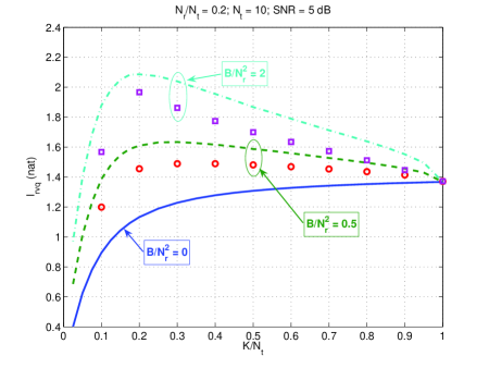
Figure 6: Mutual information per receive antenna versus normalized rank with different normalized feedback. Discrete points correspond to simulation with $N_{t}=10$.

V Quantized Precoding with Linear Receivers

In this section we evaluate the performance of a quantized precoding matrix with linear receivers (matched filter and MMSE), and compare with the performance of the optimal receiver. As $\hat{B}\to\infty$, the optimal precoding matrix eliminates the cross-coupling among channel modes, and the optimal receiver becomes the linear matched filter. Hence the corresponding achievable rates should be the same in this limit. However, for finite $\hat{B}$ the optimal receiver is expected to perform better than the linear receiver. Given a target rate, increasing the feedback therefore enables a reduction in receiver complexity.

We again assume that there are $K$ independent data streams, which are multiplexed by the linear precoder onto $N_{t}$ transmit antennas. To detect the transmitted symbols in data stream $k$, the received signal $\bm{y}$ is passed through the $N_{r}\times 1$ receive filter $\bm{c}_{k}$. The matched filter is given by

$$\bm{c}_{k}=\frac{1}{\sqrt{K}}\bm{H}\bm{v}_{k}$$ (44)

where $\bm{v}_{k}$ is the $k$th column of the precoding matrix $\bm{V}$, and the linear MMSE filter is given by

$$\bm{c}_{k}=\frac{1}{\sqrt{K}}\left(\frac{1}{K}\bm{H}\bm{V}\bm{V}^{{\dagger}}\bm{H}^{{\dagger}}+\sigma_{n}^{2}\bm{I}_{N_{r}}\right)^{-1}\bm{H}\bm{v}_{k}.$$ (45)

The SINR at the output of the linear filter $\bm{c}_{k}$ is

$$\mathrm{{\sf SINR}}_{k}=\frac{|\bm{c}_{k}^{{\dagger}}\bm{H}\bm{v}_{k}|^{2}}{\bm{c}_{k}^{{\dagger}}\left(\sum_{i\neq k}\bm{H}\bm{v}_{i}\bm{v}_{i}^{{\dagger}}\bm{H}^{{\dagger}}+K\sigma_{n}^{2}\bm{I}_{N_{r}}\right)\bm{c}_{k}}.$$ (46)

Of course, the interference among data streams can significantly decrease the channel capacity.

The performance measure is again mutual information between the transmitted symbol $x_{k}$ and the output of the filter $\bm{c}_{k}$, denoted by $\hat{x}_{k}$. In what follows, we assume independent coders and decoders for each data stream. Assuming that the interference plus noise at the output of the linear filter has a Gaussian distribution, which is true in the large system limit to be considered, the sum mutual information of all data streams per receive antenna is given by

$$R^{N_{r}} = \frac{1}{N_{r}}\sum_{k=1}^{K}I(x_{k},\hat{x}_{k})$$ (47)

$$= \frac{1}{N_{r}}\sum_{k=1}^{K}\log(1+\gamma_{k}).$$ (48)

where $\gamma_{k}$ is the SINR for the $k$th data stream. Given a channel matrix $\bm{H}$, the sum rate $R^{N_{r}}$ depends on the precoding matrix $\bm{V}$. We are interested in maximizing $R^{N_{r}}$ subject to the power constraint $\|\bm{v}_{k}\|\leq 1\mathrm{,}\ \forall k$, assuming that the power is allocated equally across streams.

Given the codebook of precoding matrices $\mathcal{V}=\{\bm{V}_{j},\ 1\leq j\leq 2^{B}\}$, the receiver selects the precoding matrix

$$\hat{\bm{V}}=\arg\max_{1\leq j\leq 2^{B}}R^{N_{r}}(\bm{V}_{j}).$$ (49)

We again consider RVQ, in which the $\bm{V}_{j}$’s are i.i.d. unitary matrices.

V-A Matched filter

Substituting (44) into (46), the SINR at the output of the matched filter is given by

$$\gamma_{k;\textsf{mf}}=\frac{(\bm{v}_{k}^{{\dagger}}\bm{H}^{{\dagger}}\bm{H}\bm{v}_{k})^{2}}{K\sigma_{n}^{2}(\bm{v}_{k}^{{\dagger}}\bm{H}^{{\dagger}}\bm{H}\bm{v}_{k})+\sum_{i=1,i\neq k}^{K}|\bm{v}_{k}^{{\dagger}}\bm{H}^{{\dagger}}\bm{H}\bm{v}_{i}|^{2}}$$ (50)

where subscript $k$ denotes the $k$th data stream. The average sum rate per receive antenna is given by

$$E_{\bm{H},\mathcal{V}}\left[\max_{1\leq j\leq 2^{B}}\{R_{\textsf{mf}}^{N_{r}}(\bm{V}_{j})=\frac{1}{N_{r}}\sum_{k=1}^{K}\log(1+\gamma_{k;\textsf{mf}})\}\right]$$ (51)

where the expectation is over the channel matrix and codebook. Since the pdf of $R_{\textsf{mf}}^{N_{r}}$ is unknown for finite $(N_{t},N_{r},K)$, we are unable to evaluate (51). Motivated by the central limit theorem, in what follows we approximate the cdf of $R_{\textsf{mf}}^{N_{r}}$ as Gaussian. The mean is taken to be the asymptotic limit

$$\mu_{\textsf{mf}}=\lim_{(N_{t},N_{r},K)\to\infty}R_{\textsf{mf}}^{N_{r}}=\frac{\bar{K}}{\bar{N}_{r}}\log\left(1+\frac{\bar{N}_{r}}{\bar{K}(1+\sigma_{n}^{2})}\right).$$ (52)

This limit follows from the fact that $\gamma_{k;\textsf{mf}}$ converges almost surely to $[\bar{K}(1+\sigma_{n}^{2})/\bar{N}_{r}]^{-1}$ as $(N_{t},N_{r},K)\to\infty$ with fixed $\bar{N}_{r}$ and $\bar{K}$. As for the optimal receiver,

$$N_{r}^{2}\mathrm{var}[R_{\textsf{mf}}^{N_{r}}|\bm{V}_{j}]\to\sigma^{2}_{\textsf{mf}}$$ (53)

where $\sigma^{2}_{mf}$ can be easily obtained by numerical simulations.

The accuracy of the Gaussian approximation for $R_{\textsf{mf}}^{N_{r}}$ is illustrated in Fig. 7, which compares the empirical pdf with the Gaussian approximation for $N_{r}=10$, $\bar{N}_{r}=1$, $K/N_{r}=0.3$ and $\mathrm{SNR}=5\,\mathrm{dB}$. The difference between the empirical and asymptotic means vanishes as $(N_{t},N_{r},K)\to\infty$.

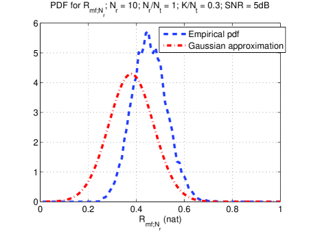
Figure 7: Comparison of the empirical pdf for $R_{\textsf{mf};N_{r}}$ with the Gaussian approximation.

We wish to apply the theory of extreme order statistics [32] to evaluate the large system limit

$$\mathcal{R}_{\textsf{rvq};\textsf{mf}}=\lim_{(N_{t},N_{r},K,B)\to\infty}[\max_{1\leq j\leq 2^{B}}R_{\textsf{mf}}^{N_{r}}(\bm{V}_{j})|\mathcal{V}].$$ (54)

Given $\mathcal{V}$, the sum rates $\{R_{\textsf{mf}}^{N_{r}}(\bm{V}_{1}),\ldots,R_{\textsf{mf}}^{N_{r}}(\bm{V}_{2^{B}})\}$ are identically distributed. However, the $R_{\textsf{mf}}^{N_{r}}(\bm{V}_{j})$’s are not independent since each depends on $\bm{H}$. This makes an exact calculation of the asymptotic rate difficult. Nevertheless, for a small number of entries in the codebook (small $B$), assuming that the rates for a given codebook are independent leads to an accurate approximation. We therefore replace the rates $R_{\textsf{mf}}^{N_{r}}(\bm{V}_{j})$, $j=1,\cdots,2^{B}$, with i.i.d. Gaussian variables with mean $\mu_{\textsf{mf}}$ and variance $\sigma^{2}_{\textsf{mf}}/N_{r}^{2}$. In analogy with the analysis of the optimal receiver in the preceding section, this gives the approximate asymptotic rate

$$\tilde{\mathcal{R}}_{\textsf{rvq};\textsf{mf}}=\mu_{\textsf{mf}}+\sigma_{\textsf{mf}}\sqrt{2\hat{B}\log 2}.$$ (55)

Numerical results, to be presented, show that this asymptotic approximation is very accurate for small to moderate values of normalized feedback $\hat{B}$. As $\hat{B}\to 0$, this approximation becomes exact. However, as $\hat{B}\to\infty$, $\tilde{\mathcal{R}}_{\textsf{rvq};\textsf{mf}}\to\infty$, whereas $\mathcal{R}_{\textsf{rvq};\textsf{mf}}$ with $\hat{B}=\infty$ is the same as the asymptotic rate with RVQ and an optimal receiver, given by (33) and (34). Hence $\mathcal{R}_{\textsf{rvq};\textsf{mf}}$ with $\hat{B}=\infty$ is finite. As for the analysis of the optimal receiver, this discrepancy is again due to the fact that the cdf of $R_{\textsf{mf}}^{N_{r}}$, which has compact support, is being approximated by a Gaussian cdf with infinite support, and also because the dependence among the sum rates $R^{N_{r}}_{\textsf{mf}}(\bm{V}_{j})$ is being ignored.

V-B MMSE receiver

Substituting (45) into (46) gives the SINR at the output of MMSE receiver for the $k$th symbol stream

$$\gamma_{k;\textsf{mmse}}=\bm{v}_{k}^{{\dagger}}\bm{H}^{{\dagger}}\left(\sum_{i\neq k}\bm{H}\bm{v}_{i}\bm{v}_{i}^{{\dagger}}\bm{H}^{{\dagger}}+K\sigma_{n}^{2}\bm{I}_{N_{r}}\right)^{-1}\bm{H}\bm{v}_{k}.$$ (56)

As for the matched filter receiver, given a codebook $\mathcal{V}$, we approximate the pdf of the instantaneous sum rate

$$R_{\textsf{mmse}}^{N_{r}}=\frac{1}{N_{r}}\sum_{k=1}^{K}\log(1+\gamma_{k;\textsf{mmse}})$$ (57)

as a Gaussian pdf with mean

$$\mu_{\textsf{mmse}}=\lim_{(N_{t},N_{r})\to\infty}R_{\textsf{mmse}}^{N_{r}}=\frac{\bar{K}}{\bar{N}_{r}}\log(1+\gamma_{\textsf{mmse}})$$ (58)

where the large system SINR is given by [30]

$$\begin{split}\gamma_{\textsf{mmse}}&=\frac{1-\bar{K}/\bar{N}_{r}}{2\sigma_{n}^{2}}-\frac{1}{2}\\ &\quad+\sqrt{\frac{(1-\bar{K}/\bar{N}_{r})^{2}}{4\sigma_{n}^{4}}+\frac{1+\bar{K}/\bar{N}_{r}}{2\sigma_{n}^{2}}+\frac{1}{4}}.\end{split}$$ (59)

As for the matched filter, the asymptotic variance $\sigma^{2}_{\textsf{mmse}}$ can be obtained via numerical simulation.

In analogy with (55), the asymptotic rate with RVQ and the MMSE receiver is given by

$$\mathcal{R}_{\textsf{rvq};\textsf{mmse}}\approx\tilde{\mathcal{R}}_{\textsf{rvq};\textsf{mmse}}=\mu_{\textsf{mmse}}+\sigma_{\textsf{mmse}}\sqrt{2\hat{B}\log 2}.$$ (60)

As for the matched filter receiver, when $\hat{B}$ is large, $\tilde{\mathcal{R}}_{\textsf{mmse}}$ over-estimates $\mathcal{R}_{\textsf{mmse}}$. For $\hat{B}=\infty$, $\mathcal{R}_{\textsf{mmse}}=\mathcal{R}_{\textsf{mf}}=\mathcal{I}_{\textsf{rvq}}$ with the optimal receiver, given by (33).

V-C Numerical Results

Fig. 8 compares the approximation for asymptotic RVQ performance with a matched filter receiver from (55) with simulated results for $N_{t}=12$, $\bar{N}_{r}=0.75$, $K/N_{t}=1/2$, and $\text{SNR}=5\,\text{dB}$. Also shown for comparison are the asymptotic rate for RVQ with an optimal receiver, derived in Section IV, the water-filling capacity ($\hat{B}=\infty$), and the rate achieved with a scalar quantizer for each coefficient. For the case shown, the analytical approximation gives an accurate estimate of the performance of the finite size system with limited feedback. The capacity with the water-filling power allocation is only slightly greater than that achieved with the on-off power allocation. The optimal receiver requires $\hat{B}\approx 0.6$ bit/dimension to achieve the capacity corresponding to unlimited feedback (33), whereas the matched filter requires $1.2$ feedback bits per dimension to reach that capacity. For other target rates, these curves illustrate the trade-off between feedback and receiver complexity.

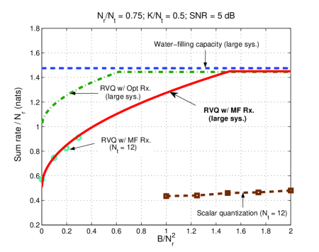
Figure 8: Sum rate per receive antenna versus normalized feedback bits with a matched filter receiver. Results are shown for RVQ (asymptotic and $N_{t}=12$) and scalar quantization. Also shown are results for the optimal receiver, and the water-filling capacity with infinite feedback.

Fig. 9 shows the same set of results as those shown in Fig. 8, but with an MMSE receiver. These results show that for the parameters selected, the MMSE receiver performs nearly as well as the optimal receiver, and requires substantially less feedback than the matched filter to achieve a target rate. Again the asymptotic approximation accurately predicts the performance of a system with a relatively small number of antennas.

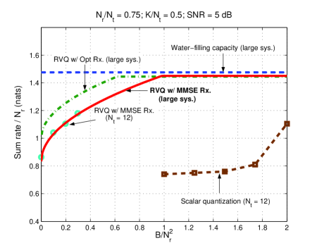
Figure 9: Sum rate per receive antenna versus normalized feedback bits with a linear MMSE receiver. Results are shown for RVQ (asymptotic and $N_{t}=12$) and scalar quantization. Also shown are results for the optimal receiver, and the water-filling capacity with infinite feedback.

VI Conclusions

We have studied the capacity of single-user MISO and MIMO fading channels with limited feedback. The feedback specifies a transmit precoding matrix, which can be optimized for a given channel realization. We first considered the performance with a rank-one precoding matrix (beamformer), and showed that the RVQ codebook is asymptotically optimal. Exact expressions for the asymptotic mutual information for MISO and MIMO channels were presented, and reveal how much feedback is required to achieve a desired performance. For the cases considered, one feedback bit for each precoder coefficient can achieve close to the water-filling capacity. Perhaps more important than the increase in capacity provided by this feedback is the associated simplification in the coding and decoding schemes that can achieve a rate close to capacity.

The performance of a precoding matrix with rank $K>1$ was also evaluated with RVQ. Although numerical examples and our beamforming results ($K=1$) suggest that RVQ is also asymptotically optimal in this case, proving this is an open problem. To compute the asymptotic achievable rate for RVQ with both optimal and linear receivers, the achievable rate with a random channel and fixed precoding matrix is approximated as a Gaussian random variable. The asymptotic rate then depends on the asymptotic mean and variance of this random variable. Although the asymptotic variance appears to be difficult to compute analytically, it can be easily obtained by simulation. Numerical results have shown that the resulting approximation accurately estimates the achievable rate with limited feedback for finite-size systems of interest.

Numerical examples comparing the performance of optimal and linear receivers have shown that the linear MMSE receiver requires little additional feedback, relative to the optimal receiver, to achieve a target rate close to the water-filling capacity. The matched filter requires significantly more feedback than the MMSE receiver (more than 0.5 bit per degree of freedom for the cases shown). At low feedback rates the achievable rate with RVQ is generally much greater than that associated with scalar quantization. Of course, this comes at a price of high complexity, since the receiver is assumed to compute the performance metric for every entry in the codebook. Other reduced complexity schemes for quantizing a beamforming vector are presented in [38, 21, 39].

Key assumptions for our results are that the channel is stationary and known at the receiver, and that the channel elements are i.i.d. Depending on user mobility and associated Doppler shifts, the channel may change too fast to allow reliable channel estimation and feedback. In that case, feedback of channel statistics, as proposed in [15, 16, 17, 18, 40], can exploit correlation among channel elements. The design of quantization codebooks for precoders, which takes correlation into account, is addressed in [40]. The effect of channel estimation error on the performance of limited feedback beamforming with finite coherence time (i.e., block fading) is presented in [41, 42].

We have also assumed that the channel gains are not frequency-selective. Limited feedback schemes for frequency-selective scalar channels are discussed in [43], and could be combined with the quantization schemes considered here. Finally, the approach presented here for a single-user MIMO channel can also be applied to multi-user models. Quantization of beamformers for the MIMO downlink have been considered in [28, 26, 27]. In that scenario the potential capacity gain due to feedback is generally much more than for the single-user channel considered here. The benefits of limited feedback for related models (e.g., frequency-selective MIMO downlink) are currently being studied.

-A Proof of Theorem 1

Given $\bm{h}$, the receiver selects the quantized beamforming vector $\hat{\bm{v}}$ to maximize the instantaneous rate in (3). Since $\log$ is monotonically increasing, the quantized beamforming vector is given by

$$\hat{\bm{v}}=\arg\max_{1\leq j\leq 2^{B}}\left\{Y_{j}=|\bm{v}_{j}^{{\dagger}}\bm{h}|^{2}/\|\bm{h}\|^{2}\right\}.$$ (61)

Since the codebook entries $\bm{v}_{j}$, $j=1,\cdots,2^{B}$, are i.i.d., the $Y_{j}$’s, given $\bm{h}$, are also i.i.d. with the cdf [25]

$$F_{Y|\bm{h}}(y)=1-(1-y)^{N_{t}-1},\quad 0\leq y\leq 1.$$ (62)

We wish to determine the distribution of $\max_{j}Y_{j}$ given $\bm{h}$. From [32, Theorem 2.1.2] it follows that

$$\frac{\max_{j}Y_{j}-a_{n}}{b_{n}}\stackrel{{\scriptstyle\mathcal{D}}}{{\longrightarrow}}\mathcal{Y}$$ (63)

where $\mathcal{Y}$ is a Weibull random variable having distribution

$$H_{\gamma}(x)=\left\{\begin{array}[]{l@{\quad}l}1,&x\geq 0\\ \exp(-(-x)^{\gamma}),&x<0\end{array}\right.,$$ (64)

$\mathcal{D}$ denotes convergence in distribution, and $a_{n}$ and $b_{n}$ are normalizing sequences, where $n=2^{B}$. Specifically, the theorem requires that $\omega(F_{Y|\bm{h}})=\sup\{y:F_{Y|\bm{h}}(y)<1\}$ be finite, and that the distribution function $F^{\ast}_{Y|\bm{h}}(y)=F_{Y|\bm{h}}(\omega(F_{Y|\bm{h}})-1/y),y>0$ satisfies, for all $y>0$,

$$\lim_{t\to\infty}\frac{1-F^{\ast}_{Y|\bm{h}}(ty)}{1-F^{\ast}_{Y|\bm{h}}(t)}=y^{-\gamma}$$ (65)

where the constant $\gamma>0$.

Substituting the expression for $F_{Y|\bm{h}}$ in (62) into (65), where $\omega(F_{Y|\bm{h}})=1$, gives

$$\lim_{t\to\infty}\frac{1-F^{\ast}_{Y|\bm{h}}(ty)}{1-F^{\ast}_{Y|\bm{h}}(t)} = \lim_{t\to\infty}\frac{\left(1/(ty)\right)^{N_{t}-1}}{\left(1/t\right)^{N_{t}-1}}$$ (66)

$$= y^{-(N_{t}-1)}$$ (67)

so that [32, Theorem 2.1.2] applies when $N_{t}>1$. Furthermore, the normalizing constants are given by

$$a_{n}=\omega(F_{Y|\bm{h}})=1$$ (68)

and

$$b_{n} = \omega(F_{Y|\bm{h}})-\inf\left\{y:1-F_{Y|\bm{h}}(y)\leq\frac{1}{n}\right\}$$ (69)

$$= 1-F^{-1}_{Y|\bm{h}}\left(1-\frac{1}{n}\right)=\left(\frac{1}{n}\right)^{\frac{1}{N_{t}-1}}.$$ (70)

To take the limit as $N_{t}\to\infty$, we will assume that the channel vector $\bm{h}$ contains the first $N_{t}$ elements of an infinite-length i.i.d. complex Gaussian vector $\bar{\bm{h}}$. Rearranging terms in (63) and taking the large system limit gives

$$\lim_{(N_{t},n)\to\infty} E_{\mathcal{V}}[\max_{j}Y_{j}|\bar{\bm{h}}]$$ (71)

$$=\lim_{(N_{t},n)\to\infty}a_{n}+b_{n}E[\mathcal{Y}]$$ (72)

$$=1-\lim_{(N_{t},n)\to\infty}\left(\frac{1}{n}\right)^{\frac{1}{N_{t}-1}}\Gamma\left(1-\frac{1}{N_{t}-1}\right)$$ (73)

$$=1-\lim_{(N_{t},B)\to\infty}2^{-\frac{B}{N_{t}-1}}$$ (74)

$$=1-2^{-\bar{B}}$$ (75)

where the gamma function $\Gamma(z)=\int_{0}^{\infty}t^{z-1}\mathrm{e}^{-t}\,\mathrm{d}t$ and we have used the fact that $E[\mathcal{Y}]=-\Gamma(1-1/(N_{t}-1))$ [44].

From (63), as $(n,N_{t})\to\infty$,

$$\mathrm{var}[\max_{j}Y_{j}|\bar{\bm{h}}]-b_{n}^{2}\mathrm{var}[\mathcal{Y}]\to 0.$$ (76)

Since $\mathrm{var}[\mathcal{Y}]=\Gamma(1-2/(N_{t}-1))-\Gamma^{2}(1-1/(N_{t}-1))\to 0$, it follows that $\mathrm{var}[\max_{j}Y_{j}|\bm{h}]\to 0$. This establishes that given $\bar{\bm{h}}$,

$$\max_{j}Y_{j}\to 1-2^{-\bar{B}}$$ (77)

in the mean square sense. The asymptotic rate difference is given by

$$\mathcal{I}_{\textsf{rvq}}^{\triangle} =\lim_{(N_{t},B)\to\infty}\left(\log(1+\rho\|\bm{h}\|^{2}\max_{1\leq j\leq 2^{B}}Y_{j})\right)-\log(\rho N_{t})$$ (78)

$$=\lim_{(N_{t},B)\to\infty}\left(\log\left(\frac{1}{\rho N_{t}}+\frac{1}{N_{t}}\|\bm{h}\|^{2}\max_{1\leq j\leq 2^{B}}Y_{j}\right)\right)$$ (79)

$$=\log(1-2^{-\bar{B}})$$ (80)

in the mean square sense, since $\|\bm{h}\|^{2}/N_{t}\to 1$ almost surely.

-B Proof of Theorem 2

The rate difference associated with codebook $\mathcal{V}_{N_{t}}$ is

$$I^{\triangle}_{\mathcal{V}_{N_{t}}} =\max_{1\leq j\leq 2^{B}}\log\left(\frac{1}{\rho N_{t}}+\frac{1}{N_{t}}|\bm{h}^{{\dagger}}\bm{v}_{j}^{N_{t}}|^{2}\right)$$ (81)

$$=\log\left(\frac{1}{\rho N_{t}}+\max_{1\leq j\leq 2^{B}}\frac{1}{N_{t}}|\bm{h}^{{\dagger}}\bm{v}_{j}^{N_{t}}|^{2}\right).$$ (82)

Taking expectation of the rate difference with respect to $\bm{h}$ and applying Jensen’s inequality, we obtain

$$E[I^{\triangle}_{\mathcal{V}_{N_{t}}}] \leq\log\left(\frac{1}{\rho N_{t}}+E[\frac{1}{N_{t}}|\bm{h}^{{\dagger}}\hat{\bm{v}}^{N_{t}}|^{2}]\right)$$ (83)

$$=\log\left(\frac{1}{\rho N_{t}}+E[\frac{1}{N_{t}}\|\bm{h}\|^{2}]E[\mu]\right)$$ (84)

where the optimal beamforming vector

$$\hat{\bm{v}}^{N_{t}}=\arg\max_{1\leq j\leq 2^{B}}|\bm{h}^{{\dagger}}\bm{v}_{j}^{N_{t}}|^{2},$$ (85)

$\mu=|\bm{h}^{{\dagger}}\hat{\bm{v}}^{N_{t}}|^{2}/\|\bm{h}\|^{2}$, and (84) follows from the fact that $\|\bm{h}\|^{2}$ and $\mu$ are independent [25].

We now derive an upper bound for $E[|\bm{h}^{{\dagger}}\hat{\bm{v}}^{N_{t}}|^{2}/\|\bm{h}\|^{2}]$ . From (30) in [2] we have

$$\begin{split}\mathrm{Pr}\{|\bm{h}^{{\dagger}}\hat{\bm{v}}^{N_{t}}|^{2}>\gamma s~{}|~{}&\|\bm{h}\|^{2}=\gamma\}\\ &\leq\left\{\begin{array}[]{l@{\quad}l}1,&0\leq s<s^{*}\\ 2^{B}(1-s)^{N_{t}-1},&s^{*}\leq s\leq 1\end{array}\right.\end{split}$$ (86)

where

$$s^{*}=1-2^{-\frac{B}{N_{t}-1}}.$$ (87)

Since the right-hand side of (86) is independent of $\gamma$, averaging over $\gamma$ gives

$$\mathrm{Pr}\{\mu>s\}\leq\left\{\begin{array}[]{l@{\quad}l}1,&0\leq s<s^{*}\\ 2^{B}(1-s)^{N_{t}-1},&s^{*}\leq s\leq 1\end{array}\right..$$ (88)

Integrating by parts, we have that

$$E[\mu] =\int_{0}^{1}\mathrm{Pr}\{\mu>x\}\,\mathrm{d}x$$ (89)

$$=\int_{0}^{s^{*}}\mathrm{Pr}\{\mu>x\}\,\mathrm{d}x+\int_{s^{*}}^{1}\mathrm{Pr}\{\mu>x\}\,\mathrm{d}x.$$ (90)

Substituting (88) into (90) and evaluating both integrals gives

$$E[\mu]\leq 1-2^{-\frac{B}{N_{t}-1}}+\frac{1}{N_{t}}2^{-\frac{B}{N_{t}-1}}.$$ (91)

Substituting $E[\|\bm{h}\|^{2}]=N_{t}$ and (91) into (84) gives

$$E[I^{\triangle}_{\mathcal{V}_{N_{t}}}]\leq\log\left(1-2^{-\frac{B}{N_{t}-1}}+\frac{1}{N_{t}}2^{-\frac{B}{N_{t}-1}}+\frac{1}{\rho N_{t}}\right)$$ (92)

and taking the large system limit gives

$$\lim_{(N_{t},B)\to\infty}E[I^{\triangle}_{\mathcal{V}_{N_{t}}}]\leq\log(1-2^{-\bar{B}}).$$ (93)

Theorem 1 states that RVQ achieves this upper bound, and therefore upper bounds the asymptotic rate difference corresponding to any quantization scheme.

-C Proof of Theorem 3

We first prove the theorem for $\bar{N}_{r}\geq 1$. Let $z=F_{\gamma|\bar{\bm{H}}}^{-1}(1-2^{-B})$. Rearranging (15) gives

$$\lim_{\begin{subarray}{c}(N_{t},N_{r})\to\infty\\ z\to\gamma_{\textsf{rvq}}^{\infty}\end{subarray}}\left[1-F_{\gamma|\bar{\bm{H}}}(z)\right]^{\frac{1}{N_{t}}}=2^{-\bar{B}}.$$ (94)

Next, we derive upper and lower bounds for the left-hand side of (94) and show that they are the same. The derivation of the upper bound is motivated by the evaluation of a similar bound for CDMA signature optimization in [34]. That is,

$$1-F_{\gamma|\bar{\bm{H}}}(z) =\Pr\left\{\left.\gamma_{j}>z\right|\bar{\bm{H}}\right\}$$ (95)

$$=\Pr\left\{\bm{v}_{j}^{{\dagger}}\bm{U}\bm{\Lambda}\bm{U}^{{\dagger}}\bm{v}_{j}>z|\bm{\Lambda},\bm{U}\right\}$$ (96)

$$=\Pr\left\{\left.\frac{\bm{w}_{j}^{{\dagger}}\bm{U}\bm{\Lambda}\bm{U}^{{\dagger}}\bm{w}_{j}}{\bm{w}_{j}^{{\dagger}}\bm{w}_{j}}>z\right|\bm{\Lambda},\bm{U}\right\}$$ (97)

where $\gamma_{j}=\frac{1}{N_{t}}\bm{v}_{j}^{{\dagger}}\bm{H}^{{\dagger}}\bm{H}\bm{v}_{j}$ and we have applied the singular value decomposition $\frac{1}{N_{t}}\bm{H}^{{\dagger}}\bm{H}=\bm{U}\bm{\Lambda}\bm{U}^{{\dagger}}$, where $\bm{U}$ is an $N_{t}\times N_{t}$ unitary matrix, $\bm{\Lambda}=\mathrm{diag}\{\lambda_{1},\cdots,\lambda_{N_{t}}\}$, and the eigenvalues are ordered as $\lambda_{1}\geq\lambda_{2}\geq\cdots\geq\lambda_{N_{t}}$. Also, $\bm{w}_{j}$ is an $N_{t}\times 1$ vector with independent, circularly symmetric, zero-mean and unit-variance Gaussian elements. Both $\bm{v}_{j}$ and $\bm{w}_{j}/\|\bm{w}_{j}\|$ are isotropically distributed, i.e., $\bm{U}\bm{w}_{j}/\|\bm{w}_{j}\|$ and $\bm{w}_{j}/\|\bm{w}_{j}\|$ have the same distribution, so that

$$1-F_{\gamma|\bar{\bm{H}}}(z) =1-F_{\gamma|\bm{\Lambda}}(z)$$ (98)

$$=\Pr\left\{\left.\frac{\sum_{i=1}^{N_{t}}\lambda_{i}w_{i}^{2}}{\sum_{i=1}^{N_{t}}w_{i}^{2}}>z\right|\bm{\Lambda}\right\}$$ (99)

$$=\Pr\left\{\left.-\sum_{i=1}^{N_{t}}(z-\lambda_{i})w_{i}^{2}>0\right|\bm{\Lambda}\right\}$$ (100)

$$=\Pr\left\{\left.-\rho\sum_{i=1}^{N_{t}}(z-\lambda_{i})w_{i}^{2}>0\right|\bm{\Lambda}\right\},\quad\forall\rho>0$$ (101)

$$=\Pr\left\{\left.\exp\left(-\rho\sum_{i=1}^{N_{t}}(z-\lambda_{i})w_{i}^{2}\right)>1\right|\bm{\Lambda}\right\}$$ (102)

where $\{w_{i}\}$ are elements of $\bm{w}_{j}$. (We omit the index $j$ to simplify the notation.) Applying Markov’s inequality and the independence of the $w_{i}$’s gives

$$1-F_{\gamma|\bm{\Lambda}}(z) \leq E_{\{w_{i}\}}\left[\exp\left\{\left.-\rho\sum_{i=1}^{N_{t}}(z-\lambda_{i})w_{i}^{2}\right\}\right|\bm{\Lambda}\right]$$ (103)

$$=\prod_{i=1}^{N_{t}}E_{w_{i}}\left[\exp\left\{-\rho(z-\lambda_{i})w_{i}^{2}\right\}|\lambda_{i}\right]$$ (104)

$$=\prod_{i=1}^{N_{t}}\int^{\infty}_{0}\exp\left\{-\rho(z-\lambda_{i})x\right\}\mathrm{e}^{-x}\mathrm{d}x$$ (105)

$$=\prod_{i=1}^{N_{t}}\int^{\infty}_{0}\exp\left\{-(1+\rho(z-\lambda_{i}))x\right\}\mathrm{d}x$$ (106)

$$=\prod_{i=1}^{N_{t}}\frac{1}{1+\rho(z-\lambda_{i})}$$ (107)

$$=\exp\left\{-\sum_{i=1}^{N_{t}}\log(1+\rho(z-\lambda_{i}))\right\}$$ (108)

when $1+\rho(z-\lambda_{i})>0$ for all $i$, or $\rho<1/(\lambda_{1}-z)$. Taking the large system limit, we obtain

$$\lim_{\begin{subarray}{c}(N_{t},N_{r})\to\infty\\ z\to\gamma_{\textsf{rvq}}^{\infty}\end{subarray}}\left[1-F_{\gamma|\bm{\Lambda}}(z)\right]^{\frac{1}{N_{t}}}\leq\exp\{-\Phi(\gamma_{\textsf{rvq}}^{\infty},\rho)\}$$ (109)

for $0<\rho<\frac{1}{\lambda_{\max}^{\infty}-\gamma_{\textsf{rvq}}^{\infty}}$, where

$$\Phi(\gamma_{\textsf{rvq}}^{\infty},\rho)\triangleq\int^{b}_{a}\log(1+\rho(\gamma_{\textsf{rvq}}^{\infty}-\lambda))g(\lambda)\mathrm{d}\lambda,$$ (110)

$g(\lambda)$ is given by (28)-(29), and $\lambda_{\max}^{\infty}=\lim_{(N_{t},N_{r})\to\infty}\lambda_{1}=(1+\sqrt{\bar{N}_{r}})^{2}$. To tighten the upper bound, we minimize (109) with respect to $\rho$, i.e.,

$$\lim_{\begin{subarray}{c}(N_{t},N_{r})\to\infty\\ z\to\gamma_{\textsf{rvq}}^{\infty}\end{subarray}}\left[1-F_{\gamma|\bm{\Lambda}}(z)\right]^{\frac{1}{N_{t}}}\leq\exp\{-\Phi(\gamma_{\textsf{rvq}}^{\infty},\rho^{*})\}$$ (111)

where

$$\rho^{*}=\arg\max_{0<\rho<\frac{1}{\lambda_{\max}^{\infty}-\gamma_{\textsf{rvq}}^{\infty}}}\Phi(\gamma_{\textsf{rvq}}^{\infty},\rho).$$ (112)

A similar expression for RVQ performance when used to quantize signatures for CDMA is derived in [34].

To derive the lower bound, we use a change of measure. (A similar approach was used in [45, Section 1.2].) Let $y_{i}\triangleq(\lambda_{i}-z)w_{i}^{2}$, which is a scaled exponential random variable with cdf $F_{i}(\cdot)$. We define the new distribution

$$G_{i}(x)\triangleq\frac{1}{M_{i}(\rho^{*})}\int_{-\infty}^{x}\mathrm{e}^{\rho^{*}y}\,\mathrm{d}F_{i}(y),$$ (113)

so that

$$M_{i}(\rho^{*})\mathrm{d}G_{i}(x)=\mathrm{e}^{\rho^{*}x}\mathrm{d}F_{i}(x),$$ (114)

where $\rho^{*}$ is given in (112), and the moment generating function for $y_{i}$ is

$$M_{i}(\theta) \triangleq E[\mathrm{e}^{\theta y_{i}}]$$ (115)

$$=\int_{0}^{\infty}\mathrm{e}^{\theta(\lambda_{i}-z)x}\mathrm{e}^{-x}\,\mathrm{d}x$$ (116)

$$=\frac{1}{1+\theta(z-\lambda_{i})}.$$ (117)

Applying the change of measure (114), we have

$$1-F_{\gamma|\bm{\Lambda}}(z)$$

$$=\Pr\{\sum_{i=1}^{N_{t}}y_{i}>0\}$$ (118)

$$=\idotsint{\bf 1}[\sum_{i=1}^{N_{t}}y_{i}>0]\,\mathrm{d}F_{1}(y_{1})\cdots\mathrm{d}F_{N_{t}}(y_{N_{t}})$$ (119)

$$=\idotsint{\bf 1}[\sum_{i=1}^{N_{t}}y_{i}>0]\mathrm{e}^{-\rho^{*}\sum_{i=1}^{N_{t}}y_{i}}\mathrm{e}^{\rho^{*}y_{1}}\mathrm{d}F_{1}(y_{1})$$ (120)

$$\qquad\cdots\mathrm{e}^{\rho^{*}y_{N_{t}}}\mathrm{d}F_{N_{t}}(y_{N_{t}})$$

$$=\prod_{i=1}^{N_{t}}M_{i}(\rho^{*})\idotsint{\bf 1}[\sum_{i=1}^{N_{t}}y_{i}>0]\mathrm{e}^{-\rho^{*}\sum_{i=1}^{N_{t}}y_{i}}\,\mathrm{d}G_{1}(y_{1})$$ (121)

$$\qquad\cdots\mathrm{d}G_{N_{t}}(y_{N_{t}})$$

where

$${\bf 1}[x>0]=\left\{\begin{array}[]{r@{\quad:\quad}l}1&x>0\\ 0&x\leq 0\end{array}\right..$$ (122)

For any $\epsilon>0$,

$$1-F_{\gamma|\bm{\Lambda}}(z)$$

$$\geq\prod_{i=1}^{N_{t}}M_{i}(\rho^{*})\idotsint{\bf 1}[\epsilon N_{t}\geq\sum_{i=1}^{N_{t}}y_{i}>0]\mathrm{e}^{-\rho^{*}\sum_{i=1}^{N_{t}}y_{i}}\,$$ (123)

$$\qquad\mathrm{d}G_{1}(y_{1})\cdots\mathrm{d}G_{N_{t}}(y_{N_{t}})$$

$$\geq\prod_{i=1}^{N_{t}}M_{i}(\rho^{*})\mathrm{e}^{-\rho^{*}\epsilon N_{t}}\idotsint{\bf 1}[\epsilon N_{t}\geq\sum_{i=1}^{N_{t}}y_{i}>0]\,$$ (124)

$$\qquad\mathrm{d}G_{1}(y_{1})\cdots\mathrm{d}G_{N_{t}}(y_{N_{t}})$$

$$=\prod_{i=1}^{N_{t}}M_{i}(\rho^{*})\mathrm{e}^{-\rho^{*}\epsilon N_{t}}\Pr\{\epsilon N_{t}\geq\sum_{i=1}^{N_{t}}\tilde{y}_{i}>0\}$$ (125)

where the $\tilde{y}_{i}$’s are independent random variables with cdf $G_{i}(\cdot)$, and the second inequality follows since $\rho^{*}>0$. To determine the probability on the right-hand side of (125), we first compute the mean of $\tilde{y}_{i}$,

$$m_{i} =\int y\,\mathrm{d}G_{i}(y)$$ (126)

$$=\frac{1}{M_{i}(\rho^{*})}\int y\mathrm{e}^{\rho^{*}y}\mathrm{d}F_{i}(y)$$ (127)

$$=(1+\rho^{*}(z-\lambda_{i}))\int_{0}^{\infty}(\lambda_{i}-z)x\mathrm{e}^{\rho^{*}(\lambda_{i}-z)x}\mathrm{e}^{-x}\,\mathrm{d}x$$ (128)

$$=\frac{\lambda_{i}-z}{1+\rho^{*}(z-\lambda_{i})}.$$ (129)

Therefore

$$\frac{1}{N_{t}}\sum_{i=1}^{N_{t}}m_{i}=\frac{1}{N_{t}}\sum_{i=1}^{N_{t}}\frac{\lambda_{i}-z}{1+\rho^{*}(z-\lambda_{i})}$$ (130)

and the asymptotic mean

$$m_{\infty} =\lim_{\begin{subarray}{c}(N_{t},N_{r})\to\infty\\ z\to\gamma_{\textsf{rvq}}^{\infty}\end{subarray}}\frac{1}{N_{t}}\sum_{i=1}^{N_{t}}m_{i}$$ (131)

$$=\int_{a}^{b}\frac{\lambda-\gamma_{\textsf{rvq}}^{\infty}}{1+\rho^{*}(\gamma_{\textsf{rvq}}^{\infty}-\lambda)}g(\lambda)\,\mathrm{d}\lambda<\infty.$$ (132)

Similarly, since $\tilde{y}_{i}$ is exponentially distributed, the variance of $\tilde{y}_{i}$ is

$$\sigma_{i}^{2}=\left(\frac{\lambda_{i}-z}{1+\rho^{*}(z-\lambda_{i})}\right)^{2}<\infty$$ (133)

and the asymptotic variance

$$\sigma_{\infty}^{2} =\lim_{\begin{subarray}{c}(N_{t},N_{r})\to\infty\\ z\to\gamma_{\textsf{rvq}}^{\infty}\end{subarray}}\frac{1}{N_{t}}\sum_{i=1}^{N_{t}}\sigma_{i}^{2}$$ (134)

$$=\int_{a}^{b}\left(\frac{\lambda-\gamma_{\textsf{rvq}}^{\infty}}{1+\rho^{*}(\gamma_{\textsf{rvq}}^{\infty}-\lambda)}\right)^{2}g(\lambda)\,\mathrm{d}\lambda<\infty.$$ (135)

Both the asymptotic mean and variance are finite.

Since the $\tilde{y}_{i}$’s are independent with finite mean and variance, the central limit theorem implies that the cdf for

$$T\triangleq\frac{\sum_{i=1}^{N_{t}}\tilde{y}_{i}-\sum_{i=1}^{N_{t}}m_{i}}{\sqrt{\sum_{i=1}^{N_{t}}\sigma^{2}_{i}}}$$ (136)

converges to a Gaussian cdf with zero mean and unit variance. Therefore we have

$$\Pr\{0<\sum_{i=1}^{N_{t}}\tilde{y}_{i}\leq\epsilon N_{t}\}$$

$$=\Pr\{-\sqrt{N_{t}}a_{N_{t}}<T\leq-\sqrt{N_{t}}a_{N_{t}}+\sqrt{N_{t}}\epsilon\frac{1}{b_{N_{t}}}\}$$ (137)

$$=F_{T}(-\sqrt{N_{t}}a_{N_{t}}+\sqrt{N_{t}}\epsilon\frac{1}{b_{N_{t}}})-F_{T}(-\sqrt{N_{t}}a_{N_{t}})$$ (138)

where $F_{T}(\cdot)$ is the cdf for $T$ and

$$a_{N_{t}}\triangleq\frac{\sum_{i=1}^{N_{t}}m_{i}/N_{t}}{\sqrt{\sum_{i=1}^{N_{t}}\sigma_{i}^{2}/N_{t}}}\to\frac{m_{\infty}}{\sigma_{\infty}},$$ (139)

$$b_{N_{t}}\triangleq\sqrt{\sum_{i=1}^{N_{t}}\sigma_{i}^{2}/N_{t}}\to\sigma_{\infty}.$$ (140)

Let $\phi(\cdot)$ denote a Gaussian cdf with zero mean and unit variance. We can rewrite (138) as

$$\begin{split}\Pr\{0<\sum_{i=1}^{N_{t}}\tilde{y}_{i}\leq\epsilon N_{t}\}=\phi(-\sqrt{N_{t}}a_{N_{t}}+\sqrt{N_{t}}\epsilon\frac{1}{b_{N_{t}}})\\ -\phi(-\sqrt{N_{t}}a_{N_{t}})+\zeta_{N_{t}}-\xi_{N_{t}}\end{split}$$ (141)

where

$$\zeta_{N_{t}} \triangleq F_{T}(-\sqrt{N_{t}}a_{N_{t}}+\sqrt{N_{t}}\epsilon\frac{1}{b_{N_{t}}})$$

$$\quad-\phi(-\sqrt{N_{t}}a_{N_{t}}+\sqrt{N_{t}}\epsilon\frac{1}{b_{N_{t}}}),$$ (142)

$$\xi_{N_{t}} \triangleq F_{T}(-\sqrt{N_{t}}a_{N_{t}})-\phi(-\sqrt{N_{t}}a_{N_{t}}).$$ (143)

Applying the Berry-Esséen theorem [46], we can bound both $\zeta_{N_{t}}$ and $\xi_{N_{t}}$ for large $N_{t}$ as

$$|\zeta_{N_{t}}|,\quad|\xi_{N_{t}}|\leq\frac{C}{\sqrt{N_{t}}}$$ (144)

where $C$ is a positive constant that depends on the variance and third moment of $\tilde{y}$. Similar to the mean and variance, we can show that the third moment is also finite.

We can now evaluate

$$\phi(-\sqrt{N_{t}}a_{N_{t}}+\sqrt{N_{t}}\epsilon\frac{1}{b_{N_{t}}})-\phi(-\sqrt{N_{t}}a_{N_{t}})$$

$$=\frac{1}{\sqrt{2\pi}}\int_{-\sqrt{N_{t}}a_{N_{t}}}^{-\sqrt{N_{t}}a_{N_{t}}+\sqrt{N_{t}}\epsilon\frac{1}{b_{N_{t}}}}\mathrm{e}^{-t^{2}/2}\,\mathrm{d}t$$ (145)

$$\leq\frac{1}{\sqrt{2\pi}}\mathrm{e}^{-N_{t}(a_{n_{t}}-\epsilon/b_{N_{t}})^{2}}\sqrt{N_{t}}\epsilon\frac{1}{b_{N_{t}}}.$$ (146)

Substituting (144) and (146) into (141), we have

$$\Pr\{0<\sum_{i=1}^{N_{t}}\tilde{y}_{i}\leq\epsilon N_{t}\}=O(1/\sqrt{N_{t}})$$ (147)

Taking the large system limit and applying L’Hopital’s rule, it follows that

$$\lim_{\begin{subarray}{c}(N_{t},N_{r})\to\infty\\ z\to\gamma_{\textsf{rvq}}^{\infty}\end{subarray}}[\Pr\{0<\sum_{i=1}^{N_{t}}\tilde{y}_{i}\leq\epsilon N_{t}\}]^{\frac{1}{N_{t}}}=1.$$ (148)

Taking the $N_{t}$th root and large system limit on both sides of (125) gives

$$\lim_{\begin{subarray}{c}(N_{t},N_{r})\to\infty\\ z\to\gamma_{\textsf{rvq}}^{\infty}\end{subarray}}\left[1-F_{\gamma|\bm{\Lambda}}(z)\right]^{\frac{1}{N_{t}}}\geq\exp\{-\Phi(\gamma_{\textsf{rvq}}^{\infty},\rho^{*})\}$$ (149)

where we use (148) and let $\epsilon\to 0$.

The lower bound in (149) is exactly the upper bound (111). Therefore,

$$\lim_{\begin{subarray}{c}(N_{t},N_{r})\to\infty\\ z\to\gamma_{\textsf{rvq}}^{\infty}\end{subarray}}\left[1-F_{\gamma|\bm{\Lambda}}(z)\right]^{\frac{1}{N_{t}}} =\exp\{-\Phi(\gamma_{\textsf{rvq}}^{\infty},\rho^{*})\}$$ (150)

$$=2^{-\bar{B}}$$ (151)

and the asymptotic RVQ received power satisfies the fixed-point equation

$$\Phi(\gamma_{\textsf{rvq}}^{\infty},\rho^{*})=\bar{B}\log(2)$$ (152)

where $\rho^{*}$ is given by (112). The goal of the rest of the proof is to simplify (152).

To determine $\rho^{*}$, we first compute

$$\frac{\partial\Phi(\gamma_{\textsf{rvq}}^{\infty},\rho)}{\partial\rho} =\int_{a}^{b}\left[\frac{\gamma_{\textsf{rvq}}^{\infty}-\lambda}{1+(\gamma_{\textsf{rvq}}^{\infty}-\lambda)\rho}\right]g(\lambda)\,\mathrm{d}\lambda$$ (153)

$$=\frac{1}{\rho}+\frac{1}{\rho^{2}}\int_{a}^{b}\frac{1}{\lambda-\underbrace{\left(\frac{1}{\rho}+\gamma_{\textsf{rvq}}^{\infty}\right)}_{y}}g(\lambda)\,\mathrm{d}\lambda$$ (154)

$$=\frac{1}{\rho}+\frac{1}{\rho^{2}}\mathcal{S}_{\bm{\Lambda}}(y)$$ (155)

where $\mathcal{S}_{\bm{\Lambda}}(\cdot)$ is the Stieltjés Transform of the asymptotic eigenvalue distribution of $\bm{\Lambda}$. Setting the derivative to zero and solving for $\rho$ gives

$$\mathcal{S}_{\bm{\Lambda}}(y)=-\rho=\frac{1}{\gamma_{\textsf{rvq}}^{\infty}-y}$$ (156)

as the only valid solution. Substituting the expression for $\mathcal{S}_{\bm{\Lambda}}$ given in [33] into (156) gives

$$\begin{split}\frac{(-1+\bar{N}_{r}-y)\pm\sqrt{y^{2}-2(\bar{N}_{r}+1)y+(\bar{N}_{r}-1)^{2}}}{2y}\\ =\frac{1}{\gamma_{\textsf{rvq}}^{\infty}-y},\end{split}$$ (157)

which simplifies to the quadratic equation

$$(\bar{N}_{r}-\gamma_{\textsf{rvq}}^{\infty})y^{2}+[\gamma_{\textsf{rvq}}^{\infty}+\bar{N}_{r}\gamma_{\textsf{rvq}}^{\infty}+(\gamma_{\textsf{rvq}}^{\infty})^{2}]y=0.$$ (158)

Solving for $y$ gives $y=0$ or $y=\gamma_{\textsf{rvq}}^{\infty}[1+1/(\gamma_{\textsf{rvq}}^{\infty}-\bar{N}_{r})]$, or equivalently, $\rho=-1/\gamma_{\textsf{rvq}}^{\infty}$ or $\rho=(\gamma_{\textsf{rvq}}^{\infty}-\bar{N}_{r})/\gamma_{\textsf{rvq}}^{\infty}$. Since $\rho>0$, we must have

$$\rho^{*}=\frac{\gamma_{\textsf{rvq}}^{\infty}-\bar{N}_{r}}{\gamma_{\textsf{rvq}}^{\infty}}.$$ (159)

Since

$$\frac{\partial^{2}\Phi(\gamma_{\textsf{rvq}}^{\infty},\rho)}{\partial\rho^{2}} =-\int_{a}^{b}\left(\frac{\lambda-\gamma_{\textsf{rvq}}^{\infty}}{1+\rho^{*}(\gamma_{\textsf{rvq}}^{\infty}-\lambda)}\right)^{2}g(\lambda)\,\mathrm{d}\lambda$$ (160)

$$<0,$$ (161)

therefore $\rho^{*}$ achieves a maximum.

By also evaluating $\Phi(\gamma_{\textsf{rvq}}^{\infty},\rho)$ at the boundary points $\rho=0$ and $\rho=1/(\lambda_{\max}^{\infty}-\gamma_{\textsf{rvq}}^{\infty})$, we have

$$\begin{split}&\rho^{*}\\ &=\left\{\begin{array}[]{l@{,\quad}l}\frac{\gamma_{\textsf{rvq}}^{\infty}-\bar{N}_{r}}{\gamma_{\textsf{rvq}}^{\infty}}&\bar{N}_{r}\leq\gamma_{\textsf{rvq}}^{\infty}\leq\bar{N}_{r}+\sqrt{\bar{N}_{r}}\\ \frac{1}{(1+\sqrt{\bar{N}_{r}})^{2}-\gamma_{\textsf{rvq}}^{\infty}}&\bar{N}_{r}+\sqrt{\bar{N}_{r}}\leq\gamma_{\textsf{rvq}}^{\infty}<(1+\sqrt{\bar{N}_{r}})^{2}\end{array}\right..\end{split}$$ (162)

To evaluate $\Phi(\gamma_{\textsf{rvq}}^{\infty},\rho^{*})$, we re-write (110) as

$$\Phi(\gamma_{\textsf{rvq}}^{\infty},\rho^{*})$$

$$=\int_{a}^{b}\left[\log(\rho^{*})+\log\left(\left(\frac{1}{\rho^{*}}+\gamma_{\textsf{rvq}}^{\infty}\right)-\lambda\right)\right]g(\lambda)\,\mathrm{d}\lambda$$ (163)

$$=\log(\rho^{*})+\int_{a}^{b}\log\left(\left(\frac{1}{\rho^{*}}+\gamma_{\textsf{rvq}}^{\infty}\right)-\lambda\right)g(\lambda)\,\mathrm{d}\lambda.$$ (164)

To evaluate the integral in (164), we apply the following Lemma.

Lemma 1.

For $x\geq(1+\sqrt{\bar{N}_{r}})^{2}$,

$$\Theta(x) \triangleq\int^{b}_{a}\log(x-\lambda)g(\lambda)\,\mathrm{d}\lambda$$ (165)

$$=\log(w(x))+\sqrt{\bar{N}_{r}}u(x)-(\bar{N}_{r}-1)\log\left(1+\frac{u(x)}{\sqrt{\bar{N}_{r}}}\right)$$ (166)

where

$$w(x) =\frac{(x-1-\bar{N}_{r})+\sqrt{(x-1-\bar{N}_{r})^{2}-4\bar{N}_{r}}}{2},$$ (167)

$$u(x) =\frac{(x-1-\bar{N}_{r})-\sqrt{(x-1-\bar{N}_{r})^{2}-4\bar{N}_{r}}}{2\sqrt{\bar{N}_{r}}}.$$ (168)

The proof of this Lemma is similar to that given in [36] and is therefore omitted here.

For $\bar{N}_{r}+\sqrt{\bar{N}_{r}}\leq\gamma_{\textsf{rvq}}^{\infty}<(1+\sqrt{\bar{N}_{r}})^{2}$, we substitute $\rho^{*}=[(1+\sqrt{\bar{N}_{r}})^{2}-\gamma_{\textsf{rvq}}^{\infty}]^{-1}$ into (164) to obtain

$$\Phi(\gamma_{\textsf{rvq}}^{\infty},[(1+\sqrt{\bar{N}_{r}})^{2}-\gamma_{\textsf{rvq}}^{\infty}]^{-1})$$ (169)

$$=-\log[(1+\sqrt{\bar{N}_{r}})^{2}-\gamma_{\textsf{rvq}}^{\infty}]+\Theta\left((1+\sqrt{\bar{N}_{r}})^{2}\right)$$ (170)

$$=-\log[(1+\sqrt{\bar{N}_{r}})^{2}-\gamma_{\textsf{rvq}}^{\infty}]+\frac{1}{2}\bar{N}_{r}\log(\bar{N}_{r})$$

$$\quad-(\bar{N}_{r}-1)\log(1+\sqrt{\bar{N}_{r}})+\sqrt{\bar{N}_{r}}$$ (171)

$$=\bar{B}\log(2).$$ (172)

Solving for $\gamma_{\textsf{rvq}}^{\infty}$ gives (18). Taking $\gamma_{\textsf{rvq}}^{\infty}=\bar{N}_{r}+\sqrt{\bar{N}_{r}}$ and solving for $\bar{B}$ gives $\bar{B}^{*}$ in (19).

For $\bar{N}_{r}\leq\gamma_{\textsf{rvq}}^{\infty}<\bar{N}_{r}+\sqrt{\bar{N}_{r}}$, or $0\leq\bar{B}\leq\bar{B}^{*}$, we substitute $\rho^{*}=\frac{\gamma_{\textsf{rvq}}^{\infty}-\bar{N}_{r}}{\gamma_{\textsf{rvq}}^{\infty}}$ into (164) to obtain

$$\begin{split}\Phi\left(\gamma_{\textsf{rvq}}^{\infty},\frac{\gamma_{\textsf{rvq}}^{\infty}-\bar{N}_{r}}{\gamma_{\textsf{rvq}}^{\infty}}\right)=\log(\gamma_{\textsf{rvq}}^{\infty}-\bar{N}_{r})-\log(\gamma_{\textsf{rvq}}^{\infty})\\ +\Theta\left(\gamma_{\textsf{rvq}}^{\infty}+\frac{\gamma_{\textsf{rvq}}^{\infty}}{\gamma_{\textsf{rvq}}^{\infty}-\bar{N}_{r}}\right).\end{split}$$ (173)

To simplify (173), we let $\psi\triangleq\gamma_{\textsf{rvq}}^{\infty}-\bar{N}_{r}$ and re-write (173) as

$$\begin{split}\Phi\left(\psi-\bar{N}_{r},\frac{\psi}{\psi+\bar{N}_{r}}\right)=\log(\psi)-\log(\psi+\bar{N}_{r})\\ +\Theta\left(1+\bar{N}_{r}+\psi+\frac{\bar{N}_{r}}{\psi}\right).\end{split}$$ (174)

After some manipulation we have

$$w\left(1+\bar{N}_{r}+\psi+\frac{\bar{N}_{r}}{\psi}\right) = \frac{\bar{N}_{r}}{\psi},$$ (175)

$$u\left(1+\bar{N}_{r}+\psi+\frac{\bar{N}_{r}}{\psi}\right) = \frac{\psi}{\sqrt{\bar{N}_{r}}},$$ (176)

and

$$\begin{split}\Theta\left(1+\bar{N}_{r}+\psi+\frac{\bar{N}_{r}}{\psi}\right)=\log(\bar{N}_{r})-\log(\psi)\\ -(\bar{N}_{r}-1)\log\left(1+\frac{\psi}{\bar{N}_{r}}\right)+\psi.\end{split}$$ (177)

Substituting (177) into (174), we obtain

$$\Phi\left(\psi-\bar{N}_{r},\frac{\psi}{\psi+\bar{N}_{r}}\right)$$

$$=\psi-\bar{N}_{r}\log\left(1+\frac{\psi}{\bar{N}_{r}}\right)$$ (178)

$$=\gamma_{\textsf{rvq}}^{\infty}-\bar{N}_{r}-\bar{N}_{r}\log(\gamma_{\textsf{rvq}}^{\infty})+\bar{N}_{r}\log(\bar{N}_{r}).$$ (179)

Setting this to $\bar{B}\log(2)$ and simplifying gives (17).

For $\bar{N}_{r}<1$, the asymptotic eigenvalue density of $\frac{1}{N_{t}}\bm{H}^{{\dagger}}\bm{H}$ is given by

$$g(\lambda)=(1-\bar{N}_{r})\delta(\lambda)+\frac{\sqrt{(\lambda-a)(b-\lambda)}}{2\pi\lambda}.$$ (180)

where $a$ and $b$ are given by (28)-(29). Following the same steps again from (110) gives (18) and (17). This completes the proof of Theorem 3.

-D Derivation of (41)-(43)

To compute $\mu_{J}$, we first write

$$J_{j}^{N_{r}}=\frac{1}{N_{r}}\sum_{k=1}^{N_{r}}\log\left(1+\rho\frac{\bar{N}_{r}}{\bar{K}}\upsilon_{k}\right)$$ (181)

where $\upsilon_{k}$ is the $k$th eigenvalue of $\bm{\Upsilon}=\frac{1}{N_{r}}\bm{H}\bm{V}_{j}\bm{V}_{j}^{{\dagger}}\bm{H}^{{\dagger}}$. As $(N_{t},N_{r},K)\to\infty$, the empirical eigenvalue distribution converges to a deterministic function $F_{\bm{\Upsilon}}(t)$. The asymptotic mean is given by

$$\mu_{J}=\lim_{(N_{t},N_{r},K)\to\infty}E[J_{j}^{N_{r}}]=\int_{0}^{\infty}\log\left(1+\rho\frac{\bar{N}_{r}}{\bar{K}}t\right)\,\mathrm{d}F_{\bm{\Upsilon}}(t).$$ (182)

A similar integral has been evaluated in [36, Eq. (6)], and the result can be directly applied to (182), giving (41).

To compute the variance, we express $J_{j}^{N_{r}}$ differently by first performing the singular value decomposition $\bm{H}=\bm{V}_{\bm{H}}\bm{\Sigma}_{\bm{H}}\bm{U}_{\bm{H}}^{{\dagger}}$, where $\bm{V}_{\bm{H}}$ is the $N_{r}\times N_{r}$ left singular matrix, $\bm{U}_{\bm{H}}$ is the $N_{t}\times N_{r}$ right singular matrix, and $\bm{\Sigma}_{\bm{H}}$ is an $N_{r}\times N_{r}$ diagonal matrix. Here we assume that $N_{t}\geq N_{r}$. (The result for $N_{t}<N_{r}$ can be shown by a similar approach.) We therefore have

$$J_{j}^{N_{r}} =\frac{1}{N_{r}}\log\det\left(\bm{I}_{N_{r}}+\rho\bm{\Lambda}\bm{L}_{j}\right)$$ (183)

$$=\frac{1}{N_{r}}\sum_{i=1}^{N_{r}}\log\left(1+\rho\eta_{i}\right)$$ (184)

where $\bm{\Lambda}=\frac{1}{K}\bm{\Sigma}^{2}_{\bm{H}}$, $\bm{L}_{j}=\bm{U}^{{\dagger}}_{\bm{H}}\bm{V}_{j}\bm{V}_{j}^{{\dagger}}\bm{U}_{\bm{H}}$, and $\eta_{i}$ is the $i$th eigenvalue of $\bm{\Lambda}\bm{L}_{j}$. To compute $\mathrm{var}[J_{j}^{N_{r}}]$, correlations between pairs of $\eta_{i}$’s are needed. Although the joint distribution of eigenvalues is known, it is complicated, so that computing the variance appears intractable.

To approximate the variance of $J_{j}^{N_{r}}$, we substitute a Taylor series expansion for $\log(1+\delta x)$ into (184) to write

$$J_{j}^{N_{r}} =\frac{\rho}{N_{r}}\sum_{i=1}^{N_{r}}\eta_{i}-\frac{\rho^{2}}{2N_{r}}\sum_{i=1}^{N_{r}}\eta_{i}^{2}+\frac{\rho^{3}}{3N_{r}}\sum_{i=1}^{N_{r}}\eta_{i}^{3}+\ldots$$ (185)

$$=\frac{\rho}{N_{r}}\mathrm{tr}\{\bm{\Lambda}\bm{L}\}-\frac{\rho^{2}}{2N_{r}}\mathrm{tr}\{(\bm{\Lambda}\bm{L})^{2}\}+\frac{\rho^{3}}{3N_{r}}\mathrm{tr}\{(\bm{\Lambda}\bm{L})^{3}\}$$

$$\quad+\ldots$$ (186)

for $\rho\eta_{\max}<1$, where $\eta_{\max}=\max_{i}\eta_{i}$, and is the maximum eigenvalue of $\bm{H}\bm{V}\bm{V}^{\dagger}\bm{H}^{\dagger}/K$. Since $\bm{H}\bm{V}$ is $N_{r}\times K$ and i.i.d., $\eta_{\max}$ has asymptotic value $(1+\sqrt{\bar{N}_{r}/\bar{K}})^{2}$. If $\bar{K}/\bar{N_{r}}=1$, then the condition asymptotically becomes $\rho<1/4$ (-6 dB). Ignoring the terms of order $\rho^{3}$ and higher, we can approximate the variance of $J_{j}^{N_{r}}$ at low SNR as

$$\mathrm{var}[J_{j}^{N_{r}}]\approx\rho^{2}\mathrm{var}\left[\frac{1}{N_{r}}\mathrm{tr}\{\bm{\Lambda}\bm{L}\}\right].$$ (187)

Letting $\bm{\Lambda}=\mathrm{diag}\{\lambda_{i}\}$ and $l_{ij}$ denote the $(i,j)$th element of $\bm{L}$, the first term in (187) can be expanded as

$$\begin{split}\mathrm{var}[\mathrm{tr}\{\bm{\Lambda}\bm{L}\}|\bm{\Lambda}]=\sum_{i=1}^{N_{r}}\lambda_{i}^{2}\left(E[l_{ii}^{2}]-E^{2}[l_{ii}]\right)\\ +\sum_{i\neq j}\lambda_{i}\lambda_{j}\left(E[l_{ii}l_{jj}]-E[l_{ii}]E[l_{jj}]\right).\end{split}$$ (188)

For a given $\bm{U}_{\bm{H}}$ and random unitary $\bm{V}$ with $K=N_{r}$, Theorem 3 in [7] states that $\bm{L}$ has a multivariate beta distribution with parameters $N_{r}$ and $N_{t}-N_{r}$. (The distribution of $\bm{L}$ is not known for general $K$.) From Theorem 2 in [47], we have

$$E[l_{ii}] =\frac{N_{r}+1}{N_{t}+2}$$ (189)

$$E[l_{ii}^{2}] =\frac{(N_{r}+1)(N_{r}+3)}{(N_{t}+2)(N_{t}+4)}$$ (190)

$$E[l_{ii}l_{jj}] =\frac{N_{r}(N_{r}+1)(N_{t}+4)+(N_{r}+1)(N_{t}-N_{r}+1)}{(N_{t}+1)(N_{t}+2)(N_{t}+4)},$$

$$\quad~{}~{}~{}i\neq j,$$ (191)

for $1\leq i,j\leq N_{r}$. Substituting (189)-(191) into (188) gives

$$\begin{split}\mathrm{var}[\mathrm{tr}\{\bm{\Lambda}\bm{L}\}|\bm{\Lambda}]=\left(\frac{1}{N_{r}}\sum_{i=1}^{N_{r}}\lambda_{i}^{2}\right)\left(\bar{N}_{r}^{2}(1-\bar{N}_{r})+O\left(\frac{1}{N_{r}}\right)\right)\\ +\left(\frac{1}{N_{r}^{2}}\sum_{i\neq j}\lambda_{i}\lambda_{j}\right)\left((\bar{N}_{r}-1)\bar{N}_{r}^{3}+O\left(\frac{1}{N_{r}}\right)\right).\end{split}$$ (192)

Taking expectation with respect to $\bm{\Lambda}$, and the large system limit, we have

$$E_{\bm{\Lambda}}\left(\mathrm{var}[\mathrm{tr}\{\bm{\Lambda}\bm{L}\}|\bm{\Lambda}]\right)\to 1-\bar{N}_{r}.$$ (193)

Also, in the large system limit

$$\frac{1}{N_{r}}\sum_{i=1}^{N_{r}}\lambda_{i}^{2} \to \int t^{2}\mathrm{d}F_{\bm{\Lambda}}(t)=\frac{1}{\bar{N}_{r}}\left(1+\frac{1}{\bar{N}_{r}}\right)$$ (194)

$$\frac{1}{N_{r}^{2}}\sum_{i\neq j}\lambda_{i}\lambda_{j} \to \left[\int t\mathrm{d}F_{\bm{\Lambda}}(t)\right]^{2}=\frac{1}{\bar{N}_{r}^{2}}$$ (195)

where $F_{\bm{\Lambda}}(t)$ is the asymptotic distribution for the diagonal elements of $\bm{\Lambda}$ or, equivalently, the asymptotic eigenvalue distribution of $\bm{H}\bm{H}^{{\dagger}}/N_{r}$.

Substituting (193) into (187), we have

$$\sigma^{2}_{J} = \lim_{(N_{r},N_{t})\to\infty}N_{r}^{2}\mathrm{var}[J_{j}^{N_{r}}]$$ (196)

$$\approx \rho^{2}(1-\bar{N}_{r}).$$ (197)

Wiroonsak Santipach (S’00-M’06) received the B.S. (summa cum laude), M.S., and Ph.D. degrees all in electrical engineering from Northwestern University, Illinois, USA in 2000, 2001, and 2006, respectively. He is currently a lecturer at the Department of Electrical Engineering, Faculty of Engineering, Kasetsart University in Bangkok, Thailand. His research interests are in wireless communications, and include performance evaluation of CDMA and MIMO system.

Michael L. Honig (S’80-M’81-SM’92-F’97) received the B.S. degree in electrical engineering from Stanford University in 1977, and the M.S. and Ph.D. degrees in electrical engineering from the University of California, Berkeley, in 1978 and 1981, respectively. He subsequently joined Bell Laboratories in Holmdel, NJ, where he worked on local area networks and voiceband data transmission. In 1983 he joined the Systems Principles Research Division at Bellcore, where he worked on Digital Subscriber Lines and wireless communications. Since the Fall of 1994, he has been with Northwestern University where he is a Professor in the Electrical Engineering and Computer Science Department. He has held visiting scholar positions at the Technical University of Munich, Princeton University, the University of California, Berkeley, Naval Research Laboratory (San Diego), and the University of Sydney. He has also worked as a free-lance trombonist. Dr. Honig has served as an editor for the IEEE Transactions on Information Theory (1998-2000), the IEEE Transactions on Communications (1990-1995), and was a guest editor for the European Transactions on Telecommunications and Wireless Personal Communications. He has also served as a member of the Digital Signal Processing Technical Committee for the IEEE Signal Processing Society, and as a member of the Board of Governors for the Information Theory Society (1997-2002). He is the recipient of a Humboldt Research Award for Senior U.S. Scientists, and the co-recipient of the 2002 IEEE Communications Society and Information Theory Society Joint Paper Award.

References

- [1] A. Narula, M. J. Lopez, M. D. Trott, and G. W. Wornell, “Efficient use of side information in multiple antenna data transmission over fading channels,” IEEE J. Select. Areas Commun., vol. 16, no. 8, pp. 1423–1436, Oct. 1998.
- [2] K. K. Mukkavilli, A. Sabharwal, E. Erkip, and B. Aazhang, “On beamforming with finite rate feedback in multiple antenna systems,” IEEE Trans. Info. Theory, vol. 49, no. 10, pp. 2562–2579, Oct. 2003.
- [3] D. J. Love and R. W. Heath, Jr., “Grassmannian beamforming for multiple-input multiple-output wireless systems,” IEEE Trans. Info. Theory, vol. 49, no. 10, pp. 2735–2745, Oct. 2003.
- [4] ——, “Limited feedback unitary precoding for spatial multiplexing systems,” IEEE Trans. Info. Theory, vol. 51, no. 8, pp. 2967–2976, Aug. 2005.
- [5] V. K. N. Lau, Y. Liu, and T.-A. Chen, “On the design of MIMO block-fading channels with feedback-link capacity constraint,” IEEE Trans. Commun., vol. 52, no. 1, pp. 62–70, Jan. 2004.
- [6] J. C. Roh and B. D. Rao, “Transmit beamforming in multiple-antenna systems with finite rate feedback: A VQ-based approach,” IEEE Trans. Info. Theory, vol. 52, no. 3, pp. 1101–1112, Mar. 2006.
- [7] ——, “Design and analysis of MIMO spatial multiplexing systems with quantized feedback,” IEEE Trans. Signal Processing, vol. 54, no. 8, pp. 2874–2886, Aug. 2006.
- [8] W. Dai, Y. Liu, V. K. N. Lau, and B. Rider, “On the information rate of MIMO systems with finite rate channel state feedback and power on/off strategy,” in Proc. IEEE Int. Symp. on Info. Theory (ISIT), Adelaide, Australia, Sept. 2005, pp. 1549–1553.
- [9] W. Dai, Y. Liu, and B. Rider, “Quantization bounds on Grassmann manifolds and applications to MIMO communications,” IEEE Trans. Inf. Theory, vol. 54, no. 3, pp. 1108–1123, Mar. 2008.
- [10] S. Zhou, Z. Wang, and G. B. Giannakis, “Quantifying the power-loss when transmit-beamforming relies on finite rate feedback,” IEEE Trans. Wireless Commun., vol. 4, no. 4, pp. 1948–1957, July 2005.
- [11] P. Xia and G. B. Giannakis, “Design and analysis of transmit-beamforming based on limited-rate feedback,” IEEE Trans. Signal Processing, vol. 54, no. 5, pp. 1853–1863, May 2006.
- [12] K. K. Mukkavilli, A. Sabharwal, and B. Aazhang, “Generalized beamforming for MIMO systems with limited transmitter information,” in Proc. Asilomar Conf. on Signals, Systems, and Computers, vol. 1, Pacific Grove, CA, Nov. 2003, pp. 1052–1056.
- [13] G. Jöngren, M. Skoglund, and B. Ottersten, “Combining beamforming and orthogonal space-time block coding,” IEEE Trans. Info. Theory, vol. 48, no. 3, pp. 611–625, Mar. 2002.
- [14] M. Skoglund and G. Jöngren, “On the capacity of a multiple-antenna communication link with channel side information,” IEEE J. Select. Areas Commun., vol. 21, no. 3, pp. 395–405, Apr. 2003.
- [15] E. Visotsky and U. Madhow, “Space-time transmit precoding with imperfect feedback,” IEEE Trans. Info. Theory, vol. 47, no. 6, pp. 2632–2639, Sept. 2001.
- [16] S. Zhou and G. B. Giannakis, “Optimal transmitter eigen-beamforming and space-time block coding based on channel mean feedback,” IEEE Trans. Signal Processing, vol. 50, no. 10, pp. 2599–2613, Oct. 2003.
- [17] S. H. Simon and A. L. Moustakas, “Optimizing MIMO antenna systems with channel covariance feedback,” IEEE J. Select. Areas Commun., vol. 21, no. 3, pp. 406–417, Apr. 2003.
- [18] S. A. Jafar and A. J. Goldsmith, “Transmitter optimization and optimality of beamforming for multiple antenna systems,” IEEE Trans. Wireless Commun., vol. 3, no. 4, pp. 1165–1175, July 2004.
- [19] P. Zador, “Asymptotic quantization error of continuous signals and the quantization dimension,” IEEE Trans. Info. Theory, vol. 28, no. 2, pp. 139–149, Mar. 1982.
- [20] R. M. Gray and D. L. Neuhoff, “Quantization,” IEEE Trans. Info. Theory, vol. 44, no. 6, pp. 2325–2383, Oct. 1998.
- [21] W. Santipach and M. L. Honig, “Signature optimization for CDMA with limited feedback,” IEEE Trans. Info. Theory, vol. 51, no. 10, pp. 3475–3492, Oct. 2005.
- [22] D. J. Love, R. W. Heath, Jr., W. Santipach, and M. L. Honig, “What is the value of limited feedback for MIMO channels?” IEEE Commun. Mag., vol. 42, no. 10, pp. 54–59, Oct. 2004.
- [23] S. Bhashyam, A. Sabharwal, and B. Aazhang, “Feedback gain in multiple antenna systems,” IEEE Trans. Commun., vol. 50, no. 5, pp. 785–798, May 2002.
- [24] V. K. N. Lau, Y. Liu, and T.-A. Chen, “Role of transmit diversity for wireless communications – reverse link analysis with partial feedback,” IEEE Trans. Commun., vol. 50, no. 12, pp. 2082–2090, Dec. 2002.
- [25] C. K. Au-Yeung and D. J. Love, “On the performance of random vector quantization limited feedback beamforming,” IEEE Trans. Wireless Commun., vol. 6, no. 2, pp. 458–462, Feb. 2005.
- [26] N. Jindal, “MIMO broadcast channels with finite-rate feedback,” IEEE Trans. Info. Theory, vol. 52, no. 11, pp. 5045–5060, Nov. 2006.
- [27] T. Yoo, N. Jindal, and A. Goldsmith, “Multi-antenna downlink channels with limited feedback and user selection,” IEEE J. Select. Areas Commun., vol. 25, no. 7, pp. 1478–1491, Sep. 2007.
- [28] M. Sharif and B. Hassibi, “On the capacity of MIMO broadcast channel with partial side information,” IEEE Trans. Info. Theory, vol. 51, no. 2, pp. 506–522, Feb. 2005.
- [29] P. Viswanath, D. N. C. Tse, and R. Laroia, “Opportunistic beamforming using dumb antennas,” IEEE Trans. Info. Theory, vol. 48, no. 6, pp. 1277–1294, June 2002.
- [30] D. N. C. Tse and O. Zeitouni, “Linear multiuser receivers in random environments,” IEEE Trans. Info. Theory, vol. 46, no. 1, pp. 171–188, Jan. 2000.
- [31] L. Zheng and D. N. C. Tse, “Diversity and multiplexing: A fundamental tradeoff in multiple-antenna channels,” IEEE Trans. Info. Theory, vol. 49, no. 5, pp. 1073–1096, May 2003.
- [32] J. Galambos, The Asymptotic Theory of Extreme Order Statistics, 2nd ed. Robert E. Krieger, 1987.
- [33] V. A. Marc̆enko and L. A. Pastur, “Distribution of eigenvalues for some sets of random matrices,” Math. USSR-Sbornik, vol. 1, pp. 457–483, 1967.
- [34] W. Dai, Y. Liu, and B. Rider, “Performance analysis of CDMA signature optimization with finite rate feedback,” in Proc. Conf. on Info. Sciences and Systems (CISS), Princeton, NJ, Mar. 2006.
- [35] İ. E. Telatar, “Capacity of multi-antenna Gaussian channels,” European Trans. on Telecommun., vol. 10, pp. 585–595, Nov. 1999.
- [36] P. B. Rapajic and D. Popescu, “Information capacity of a random signature multiple-input multiple-output channel,” IEEE Trans. Commun., vol. 48, no. 8, pp. 1245–1248, Aug. 2000.
- [37] Z. D. Bai and J. W. Silverstein, “CLT for linear spectral statistics of large dimensional sample covariance matrices,” Annals of Probability, vol. 32, no. 1A, pp. 553–605, 2004.
- [38] W. Santipach and M. L. Honig, “Signature optimization for DS-CDMA with limited feedback,” in Proc. IEEE Int. Symp. on Spread-Spectrum Tech. and Appl. (ISSSTA), Prague, Czech Republic, Sept. 2002, pp. 180–184.
- [39] D. J. Ryan, I. V. L. Clarkson, I. B. Collings, D. Guo, and M. L. Honig, “QAM and PSK codebooks for limited feedback MIMO beamforming,” to appear in IEEE Trans. on Commun., Feb. 2009.
- [40] V. Raghavan, R. W. Heath, Jr., and A. M. Sayeed, “Systematic codebook designs for quantized beamforming in correlated MIMO channels,” IEEE J. Select. Areas Commun., vol. 25, no. 7, pp. 1298–1310, Sept. 2006.
- [41] W. Santipach and M. L. Honig, “Capacity of beamforming with limited training and feedback,” in Proc. IEEE Int. Symp. on Info. Theory (ISIT), Seattle, WA, July 2006.
- [42] ——, “Optimization of training and feedback for beamforming over a MIMO channel,” in Proc. IEEE Wireless Commun. and Networking Conf. (WCNC), Hong Kong, China, Mar. 2007.
- [43] Y. Sun and M. L. Honig, “Asymptotic capacity of multicarrier transmission with frequency-selective fading and limited feedback,” IEEE Trans. Info. Theory, vol. 54, no. 7, pp. 2879–2902, July 2008.
- [44] E. Castillo, Extreme Value Theory in Engineering. Academic Press, 1988.
- [45] A. Shwartz and A. Weiss, Large Deviations for Performance Analysis. Queues, Communications, and Computing. London, UK: Chapman & Hall, 1995.
- [46] J. K. Patel and C. B. Read, Handbook of the Normal Distribution, 2nd ed., ser. Statistics: a Series of Textbooks and Monographs. New York: Marcel Dekker, 1996.
- [47] C. G. Khatri and K. C. S. Pillai, “Some results on the non-central multivariate Beta distribution and moments of traces of two matrices,” Annals of Mathematical Statistics, vol. 36, no. 5, pp. 1511–1520, Oct. 1965.