FRACTIONALLY CHARGED EXCITATIONS ON FRUSTRATED LATTICES

Abstract

Systems of strongly correlated fermions on certain geometrically frustrated lattices at particular filling factors support excitations with fractional charges $\pm e/2$. We calculate quantum mechanical ground states, low–lying excitations and spectral functions of finite lattices by means of numerical diagonalization. The ground state of the most thoroughfully studied case, the criss-crossed checkerboard lattice, is degenerate and shows long–range order. Static fractional charges are confined by a weak linear force, most probably leading to bound states of large spatial extent. Consequently, the quasi-particle weight is reduced, which reflects the internal dynamics of the fractionally charged excitations. By using an additional parameter, we fine–tune the system to a special point at which fractional charges are manifestly deconfined—the so–called Rokhsar–Kivelson point. For a deeper understanding of the low–energy physics of these models and for numerical advantages, several conserved quantum numbers are identified.

I Introduction

Quantization of charge is a very basic feature in the description of the physical world. Therefore, fractionally charged excitations came as a surprise to physicists. Already back in the year 1979, Su, Schrieffer, and Heeger su1979 showed that a model describing the one-dimensional (1D) chain molecule trans–polyacetylene $\mathrm{(CH)_{n}}$ supports excitations with spin–charge separation. This is not yet charge fractionalization, but when the model is considered at different electron densities (corresponding to extremely high doping), it turns out that at certain filling factors elementary excitations with fractional charge exist [in the simplest case $q=\pm e/3\$and $q=\pm 2e/3$]. A few years later, Laughlin laughlin1983 interpreted the much celebrated fractional quantum Hall effect (FQHE) in terms of fractionally charged (quasi-) particles (fcp) and fractionally charged (quasi-) holes (fch). Thereby, he firmly established the idea of fractional charges in our understanding of solid–state physics. Direct electron–electron interactions are crucial in the FQHE: Correlations become strong in an applied magnetic field because the kinetic energy of the electrons is quenched. Of course, no one will ever extract a fraction of an electron from an FQHE sample. But thinking of an extra electron or an extra hole near fill factor $\nu=1/3$ as decaying into three separate entities of charge $q=\pm e/3\$each proved enormously helpful for a qualitative and quantitative understanding of the FQHE—and was rewarded by the Nobel Prize in Physics 1998.

The question was left open whether or not fractionally charged excitations exist in 2D or 3D systems without a magnetic field. In 2002, it was suggested by one of us fulde2002 that excitations with charge $\pm e/2$ do exist in certain 2D and 3D lattices, e.g., the pyrochlore lattice, which is a prototype 3D structure with geometrical frustration. The original work was motivated by the transition metal compound $\mathrm{LiV_{2}O_{4}}$, which surprisingly shows heavy–fermion behavior with, e.g., a large $\gamma$ coefficient in the low-temperature specific heat $C=\gamma T$.kondo1997 However, we will not address the issue whether the models discussed here apply to any particular material or artifical systems such as optical lattices, see e.g. Ref. hofstetter2002 and citations therein. Instead, we try to contribute to the very general question whether or not fractional charges can exist at all in truly 2D or 3D systems in the absence of magnetic fields.

We would like to argue that general prerequisites for fractional charges are—as in the FQHE case—strong short–range correlations and certain band fillings. Furthermore, the short–range correlations should be somehow incompatible with the lattice structure in order to prevent the development of long–range order. Following the general usage, we will simply call the lattice “frustrated” even though calling the interaction “frustrated by the lattice” would be the more accurate terminology.

In this contribution, we study the charge degrees of freedom on such lattices systematically and consider a class of models of strongly correlated spinless fermions. Most of our numerical calculations were done for the 2D checkerboard lattice, which is easier to deal with than the even more interesting 3D cases. For future work, one can hope to learn from comparison with spin systems where numerous studies exist for the pyrochlore lattice and its 2D relatives, the crisscrossed checkerboard lattice and the kagome lattice.misguich2003 ; diep2005 ; hermele2004 ; lauchli2004 ; shannon2004

II Fractional charges on frustrated lattices

(a)

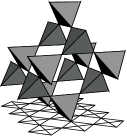
(b)

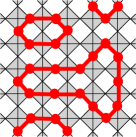
(c)

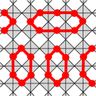
Figure 1: (a) Checkerboard lattice as 2D projection of the 3D pyrochlore lattice. moessner2004 (b,c) Two examples of allowed configurations on a checkerboard lattice at half filling. Occupied sites are connected by thick lines as guides to the eye.

In order to illustrate the concept of fractional charges on frustrated lattices, we focus here on the (crisscrossed) 2D checkerboard lattice. Figure 1(a) illustrates that the checkerboard lattice can be thought of as a projection of the pyrochlore lattice onto a plane. In the following, we adopt the ideas of Ref. fulde2002 and consider a model Hamiltonian of spinless fermions

$$H=-t\sum_{\langle i,j\rangle}\left(c_{i}^{{\dagger}}c_{j}^{\vphantom{{\dagger}}}+\mbox{H.c.}\right)+V\sum_{\langle i,j\rangle}n_{i}n_{j}$$ (1)

on a checkerboard lattice. The operators $c_{i}^{\vphantom{{\dagger}}}(c_{i}^{{\dagger}})$ annihilate (create) fermions on sites $i$. The density operators are $n_{i}=c_{i}^{{\dagger}}c_{i}^{\vphantom{{\dagger}}}$. We assume half filling, $\sum_{i}n_{i}=\frac{N}{2}$ for a system with $N$ sites. Our main interest is the regime where the nearest–neighbor hopping $t$ is much smaller than the nearest–neighbor repulsion $V$, i.e., $|t|/V\ll 1$. Henceforth, we assume $t>0$. In analogy to the tetrahedra in a pyrochlore lattice, all bonds in a crossed square are equivalent.

Classical correlations and ground–state degeneracy.

For a moment, let us set the hopping–matrix element $t$ to zero. The ground–state manifold is then macroscopically degenerate: Every configuration that satisfies the so–called tetrahedron rule of having exactly two particles on each tetrahedron (crisscrossed square) is a (classical) ground state anderson1956 and will henceforth be referred to as an “allowed configuration.” Examples are shown in Fig. 1(b) and (c). Note that our coordinate system is rotated by $45^{\circ}$ relative to that of, e.g., Ref. runge2004 . The resulting difference in boundary conditions can lead to noticeable numerical differences in particular for small cluster sizes.

One can visualize the origin of the macroscopic degeneracy as follows: Take the set of the six allowed crisscrossed squares and construct row by row a larger allowed configuration. Whenever a crisscrossed square is added, we can choose between one, two, or three different possibilities, depending on the neighboring crisscrossed squares. Since there often is a choice to make, an exponential number of different allowed configurations can be constructed. Thus, the system has a finite entropy at $T=0$. The exact value of the ground-state degeneracy can be obtained from a mapping to the so–called six–vertex model. baxter1982 Its solution is highly non–trivial due to the existence of long–range correlations, which seem to be a generic feature seen in many frustrated lattice models.pollmann2006a

All classical ($t=0$) ground states have the important property of being incompressible in the sense that no fermion can hop to another empty site without creating defects and thereby increasing the repulsion energy. In other words, we have to violate the tetrahedron rule in intermediate states if we want to connect via hopping processes one allowed configuration with another.

Fractional charges.

(a)

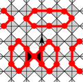
(b)

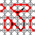
(c)

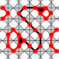
Figure 2: (a) Adding one fermion to the half–filled checkerboard lattice leads to two defects (marked by black triangles) on adjacent crisscrossed squares. (b), (c) Two defects with charge $e/2$ can separate without creating additional defects. They are connected by a string consisting of an odd number of fermions.

Placing one additional particle with charge $e$ onto an empty site of an allowed configuration leads to a violation of the tetrahedron rule on two adjacent crisscrossed squares, see Fig. 2(a). The energy is increased by $4V$ since the added particle has four nearest neighbors (charge gap). There is no way to remove the violations of the tetrahedron rule by moving electrons. However, fermions on a crisscrossed square with three particles can hop to another neighboring crisscrossed square without creating additional violations of the tetrahedron rule, i.e., without increase of the repulsion energy [see Fig. 2(b,c)]. By these hopping processes, two local defects (violations of the tetrahedron rule) can separate and the added fermion with charge $e$ breaks into two pieces. They carry a fractional charge of $e/2$ each. In the quantum mechanical case ($t\not=0$), the separation leads to a lowering of the kinetic energy of order $|t|$.

Energy and momentum must be conserved by the decay processes $1e\rightarrow 2\mathrm{fcp^{\prime}s}$. If we associate momentum $\mathbf{k}$ and energy $E(\mathbf{k})$ with the inserted fermion, they must now be shared between the resulting two fcp’s into which it has decayed

$$E\left(\mathbf{k}\right)=4V+\epsilon\left(\mathbf{k}_{1}\right)+\epsilon\left(\mathbf{k}_{2}\right).$$ (2)

Here $\mathbf{k}=\mathbf{k}_{1}+\mathbf{k}_{2}$ and $\epsilon\left(\mathbf{k}\right)$ is the energy dispersion of a fcp. Even though $\epsilon\left(\mathbf{k}\right)$ is at present completely unknown, Eq. (2) allows to predict that for deconfined fcp’s the electronic spectral function should not contain a Fermi–liquid peak, but should show a broad continuum instead.

Figure 2 demonstrates that the two defects can be thought of as always being connected by a string of occupied sites consisting of an odd number of sites. The fractional charges can thus be alternatively interpreted as the ends of a string–like excitation. In this picture, the connection is not static, as two pairs of fcp’s can exchanges partners when the connecting strings come close.

Quantum Fluctuations.

(a)

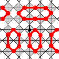
(b)

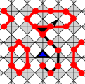
(c)

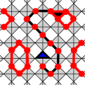
(d)

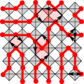
Figure 3: (a)–(c) Hopping of a fermion to a neighboring site in an allowed configuration generates a fluctuation: (a) A fractional charged particle (fcp) and fractional charged hole (fch) are generated. (b)–(c) The two defect (marked by triangles) with charge $\pm e/2$ can separate without creating additional defects and are connected by a string consisting of an even number of fermions. (d) Example of an allowed configuration on a checkerboard lattice at half filling with possible low–order hopping processes.

If we relax the constraint of having two fermions on each crisscrossed square and consider a small but finite ratio $t/V,$ quantum fluctuations come into play. The quantum fluctuations lead also to fractional charges, but do not change the net charge of the systems. Starting from an allowed configuration, the hopping of a fermion to a neighboring site increases the energy by $V$. One crisscrossed square contains three fermions while the other has only one fermion, see Fig. 3(a)–(c). These so-called vacuum fluctuations (virtual fcp–fch pairs) lead to two mobile fractional charges with opposite charges $+e/2$ and $-e/2$, which are connected by a string of an even number of fermions. The energy associated with a free fcp and a free fch is $\Delta E_{\mbox{vac}}=V+\epsilon\left(\mathbf{k}\right)+\bar{\epsilon}\left(-\mathbf{k}\right)$, where $\bar{\epsilon}\left(-\mathbf{k}\right)$ denotes the kinetic energy of a fch. Such virtual processes connect different allowed configurations, lower the total energy, and reduce the macroscopic degeneracy, as we will see more explicitely in the next section.

Fractional charges in 3D.

(a)

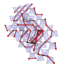
(b)

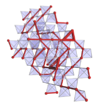
Figure 4: Adding one fermion to the half–filled three-dimensional pyrochlore lattice leads to two defects on adjacent tetrahedra. The two defects with charge $e/2$ can separate without creating additional defects and are connected by a string consisting of an odd number of fermions.

All arguments mentioned above for the existence of fcp’s on a 2D checkerboard lattice can be directly transferred to a 3D pyrochlore lattice at half filling, see Fig. 4. Fcp’s correspond to tetrahedra with three fermions and fch’s to tetrahedra with only one fermion.

III Effective Hamiltonians

Ring exchange processes in the undoped case.

The numerical and analytical work is greatly simplified, if a simpler Hamiltonian $\mathcal{H}$ can be derived that shows in the limit $|t|\ll V$ the same low–energy physics as the model Hamiltonian (1). A down–folding procedure can be used to define $\mathcal{H}$: Per definition, it acts only on the subspace of allowed configurations and includes all virtual processes up to the lowest non–trivial order, which is $t^{3}/V^{2}$. The relevant processes are shown in see Fig. 3(d) and can be classified as self–energy contributions $H_{\Sigma}$ and ring–exchange processes $H_{\mathrm{eff}}$, $\mathcal{H}=H_{\Sigma}+H_{\mathrm{eff}}$. The former comprises the terms which are diagonal in the real space basis. The latter includes those which connect different allowed configurations. $H_{\Sigma}$ contains fermion hops to an empty neighboring site and back again as well as hops around an adjacent triangle. These contribute only a constant, configuration–independent energy shift. It does not lift the macroscopic degeneracy and will hence be ignored furtheron. The total amplitude of ring–exchange processes around empty squares is proportional to $t^{2}/V$. It vanishes for spinless fermions because the amplitudes for clockwise and counter–clockwise ring–exchange cancel each other due to fermionic anti–commutation relations. Thus, the macroscopic ground–state degeneracy is first lifted by ring exchanges $\sim t^{3}/V^{2}$ around hexagons, and the looked–for effective Hamiltonian reads

$$H_{\mathrm{eff}} = -g{\textstyle\sum_{\{\psset{unit=19.91693pt}\pspicture[0.2](7.96677pt,3.98338pt)\psset{linewidth=0.5975pt,linestyle=solid}{\psset{}\pspolygon(0.0pt,1.99168pt)(1.99168pt,0.0pt)(5.97507pt,0.0pt)(7.96677pt,1.99168pt)(5.97507pt,3.98338pt)(1.99168pt,3.98338pt)}\endpspicture\;,\;\psset{unit=19.91693pt}\pspicture[0.15](3.98338pt,6.97092pt)\psset{linewidth=0.5975pt,linestyle=solid}{\psset{}\pspolygon(1.99168pt,-1.99168pt)(0.0pt,0.0pt)(0.0pt,3.98338pt)(1.99168pt,5.97507pt)(3.98338pt,3.98338pt)(3.98338pt,0.0pt)}\endpspicture\;\}}}\big{(}\,\big{|}\;\psset{unit=19.91693pt}\pspicture[0.2](19.91693pt,9.95847pt)\psset{linewidth=0.5975pt,linestyle=solid}{\psset{}\pspolygon(0.0pt,4.97923pt)(4.97923pt,0.0pt)(14.9377pt,0.0pt)(19.91693pt,4.97923pt)(14.9377pt,9.95847pt)(4.97923pt,9.95847pt)}\psset{linewidth=0.5975pt,linestyle=solid}{\psset{fillcolor=lightgray,fillstyle=solid}\pspolygon(4.97923pt,0.0pt)(14.9377pt,0.0pt)(9.95847pt,4.97923pt)}{\psset{fillcolor=lightgray,fillstyle=solid}\pspolygon(4.97923pt,9.95847pt)(14.9377pt,9.95847pt)(9.95847pt,4.97923pt)}{\psset{}\psline(9.95847pt,0.0pt)(9.95847pt,9.95847pt)}\psset{linewidth=1.59335pt,linestyle=solid}{\psset{linecolor=black,dotsize=2.98753pt 0.0}\psdots(4.97923pt,0.0pt)(4.97923pt,9.95847pt)(19.91693pt,4.97923pt)(9.95847pt,4.97923pt)}\endpspicture\;\big{\rangle}\big{\langle}\;\psset{unit=19.91693pt}\pspicture[0.2](19.91693pt,9.95847pt)\psset{linewidth=0.5975pt,linestyle=solid}{\psset{}\pspolygon(0.0pt,4.97923pt)(4.97923pt,0.0pt)(14.9377pt,0.0pt)(19.91693pt,4.97923pt)(14.9377pt,9.95847pt)(4.97923pt,9.95847pt)}\psset{linewidth=0.5975pt,linestyle=solid}{\psset{fillcolor=lightgray,fillstyle=solid}\pspolygon(4.97923pt,0.0pt)(14.9377pt,0.0pt)(9.95847pt,4.97923pt)}{\psset{fillcolor=lightgray,fillstyle=solid}\pspolygon(4.97923pt,9.95847pt)(14.9377pt,9.95847pt)(9.95847pt,4.97923pt)}{\psset{}\psline(9.95847pt,0.0pt)(9.95847pt,9.95847pt)}\psset{linewidth=1.59335pt,linestyle=solid}{\psset{linecolor=black,dotsize=2.98753pt 0.0}\psdots(0.0pt,4.97923pt)(14.9377pt,0.0pt)(14.9377pt,9.95847pt)(9.95847pt,4.97923pt)}\endpspicture\;\big{|}-\big{|}\;\psset{unit=19.91693pt}\pspicture[0.2](19.91693pt,9.95847pt){\psset{linecolor=black,dotsize=2.98753pt 0.0}\psdots(4.97923pt,0.0pt)(4.97923pt,9.95847pt)(19.91693pt,4.97923pt)}\psset{linewidth=0.5975pt,linestyle=solid}{\psset{}\pspolygon(0.0pt,4.97923pt)(4.97923pt,0.0pt)(14.9377pt,0.0pt)(19.91693pt,4.97923pt)(14.9377pt,9.95847pt)(4.97923pt,9.95847pt)}\psset{linewidth=0.5975pt,linestyle=solid}{\psset{fillcolor=lightgray,fillstyle=solid}\pspolygon(4.97923pt,0.0pt)(14.9377pt,0.0pt)(9.95847pt,4.97923pt)}{\psset{fillcolor=lightgray,fillstyle=solid}\pspolygon(4.97923pt,9.95847pt)(14.9377pt,9.95847pt)(9.95847pt,4.97923pt)}{\psset{}\psline(9.95847pt,0.0pt)(9.95847pt,9.95847pt)}\psset{linewidth=1.59335pt,linestyle=solid}\endpspicture\;\big{\rangle}\big{\langle}\;\psset{unit=19.91693pt}\pspicture[0.2](19.91693pt,9.95847pt){\psset{linecolor=black,dotsize=2.98753pt 0.0}\psdots(0.0pt,4.97923pt)(14.9377pt,0.0pt)(14.9377pt,9.95847pt)}\psset{linewidth=0.5975pt,linestyle=solid}{\psset{}\pspolygon(0.0pt,4.97923pt)(4.97923pt,0.0pt)(14.9377pt,0.0pt)(19.91693pt,4.97923pt)(14.9377pt,9.95847pt)(4.97923pt,9.95847pt)}\psset{linewidth=0.5975pt,linestyle=solid}{\psset{fillcolor=lightgray,fillstyle=solid}\pspolygon(4.97923pt,0.0pt)(14.9377pt,0.0pt)(9.95847pt,4.97923pt)}{\psset{fillcolor=lightgray,fillstyle=solid}\pspolygon(4.97923pt,9.95847pt)(14.9377pt,9.95847pt)(9.95847pt,4.97923pt)}{\psset{}\psline(9.95847pt,0.0pt)(9.95847pt,9.95847pt)}\psset{linewidth=1.59335pt,linestyle=solid}\endpspicture\;\big{|}+\mbox{H.c.}\,\big{)},$$ (3)

with the effective hopping–matrix element $g=12\ t^{3}/V^{2}>0$ and the sum taken over all vertical and horizontal oriented hexagons. The pictographic operators represent the hopping around hexagons which have either an empty or an occupied central site. The signs of the matrix elements depend on the representation and the sequence in which the fermions are ordered. When the sites are enumerated along diagonal rows, an exchange process commutes an odd number of fermionic operators if the site in the center of the hexagon is empty and an even number if the center is occupied. In Ref. runge2004 , it has been shown that the effective Hamiltonian (3) gives a good approximation of the low–energy excitations of the full Hamiltonian (1) in the limit considered.

Propagation of defects and extra charges.

We have derived $H_{\mathrm{eff}}$ as effective Hamiltonian for local rearrangement processes as resulting from the (virtual/intermediate) generation of a defect pair which subsequently recombines, leaving behind a different allowed generation. For many questions of physical interest, it is necessary to consider the propagation of defects over large distances. Analogously to conventional semiconductors, this refers to long–lived thermally generated defects (e–h pairs in the semiconductor analogy) as well as to the consequences of slight doping, i.e., addition of two fcp’s by addition of one extra fermion. The natural generalization of the effective Hamiltonian (3) to these cases includes besides the lowest order ring–exchange processes $H_{\mathrm{eff}}$ a projected hopping term that moves the defects

$$H_{\mathrm{tg}} = H_{\mathrm{eff}}-t\sum_{\langle i,j\rangle}P\left(c_{i}^{{\dagger}}c_{j}^{\vphantom{{\dagger}}}+\mbox{H.c.}\right)P.$$ (4)

The projector $P$ ensures that $H_{\mathrm{tg}}$ acts only on the subspace of configurations with the smallest possible number of violations of the tetrahedron rule which is compatible with the number of particles, e.g., two in the case of one added fermion. We refer to $H_{\mathrm{tg}}$ as the $t$–$g$ model and consider the parameters $t$ and $g$ as independent (i.e., not restricted to the regime $g\ll t$ as enforced by $t\ll V$). This allows to study the effect of ring exchange onto the dynamics of fractionally charged excitations. In particular, the question of confinement can be studied even on rather small clusters by increasing the ring exchange strength $g$ relative to $t$.

IV Height representation, conserved quantities, and gauge symmetries

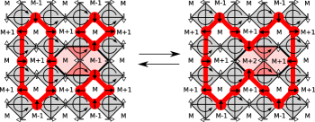
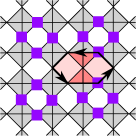
(a)	(b)	(c)

Figure 5: (a) Height representation for examples of allowed configurations of a $\sqrt{32}\times\sqrt{32}$ checkerboard lattice with periodic boundary conditions at half filling. The height field $h$ (numbers in the non–crossed squares) is uniquely defined for a given configuration up to an additive constant $M$. The field $\mathbf{f}=\nabla h$ is indicated by small arrows on the lattice sites. Details of the mapping can be found in the text. The effect on the height fields of a ring–exchange process around a hexagon is shown explicitely. (b) The effective Hamiltonian conserves the number of fermions on each of the four sublattices of the checkerboard lattice which are labeled by “blue squares”, “red circles”, “yellow stars” and “green triangles.” (c) Ring–exchange processes change the number of fermions on sites marked by dark “purple squares” by two.pollmannDissertation

Conserved quantities of a Hamiltonian allow for a reduction of the numerical effort by exploiting the resulting block–diagonal form of the matrix representation. The real space configurations spanning the subspaces corresponding to these blocks will be referred to as “subensembles.” Eigenstates can conveniently be classified by the eigenvalues of the conserved quantities as quantum numbers for our model. We will now identify several such quantum numbers in order to characterize different subensembles. A topological quantity, which is conserved by all local processes, i.e., ring–exchange processes, is the average tilt of a scalar height field which will be introduced in the next paragraph. Another useful set of quantum numbers are the number $(N_{\mathcal{B}},N_{\mathcal{Y}},N_{\mathcal{G}},N_{\mathcal{R}})$ of particles on the four sublattices referred to as blue, yellow, green and red as shown in Fig. 5(b). They are conserved by $H_{\mathrm{eff}}$.

Any allowed configurations of the half–filled checkerboard can uniquely be represented by a vector field $\mathbf{f}$ for which the discretized lattice version of the (discrete) curl vanishes, i.e., a pure (discrete) gradient of a scalar field (height field) $\mathbf{f}=\nabla h$, see Fig. 5. The height field $h,$ is derived from the local constraint expressed by the tetrahedron rule as follows: A clockwise or counter–clockwise orientation is assigned alternatingly to the crisscrossed squares. Arrows of unit length are placed on the lattice sites. The arrows point along (against) the orientation of the adjacent crisscrossed squares if the site is occupied (empty). It is easily checked that allowed configurations are those for which the discretized line integral of $\mathbf{f}$ around every closed loop vanishes. Thus, $\mathbf{f}=\nabla h$ defines a height field $h$ up to an arbitrary constant $M$.

The height at the upper (right) and at the lower (left) boundary of a finite lattice of $N_{x}\times N_{y}$ squares with periodic boundary conditions can differ only by an integer $-N_{y(x)}\leq\kappa_{y(x)}\leq N_{y(x)}$, which is the same for all columns (rows). This defines topological quantum numbers $(\kappa_{x},\kappa_{y})$. They remain unchanged by all local processes that transform one allowed configuration into another, i.e., by ring–exchange processes along contractible loops. In particular, $H_{\mathrm{eff}}$ merely lowers or raises the local height of two adjacent plain squares by $\pm 2$, as illustrated in Fig. 5(a). We refer to $(\kappa_{x}/N_{x},\kappa_{y}/N_{y})$ as global slope.

The lattice symmetry is broken for states with $(\kappa_{x},\kappa_{y})\neq(0,0)$:runge2004 E.g., a finite positive value of $\kappa_{x}/N_{x}$ implies a charge modulation along diagonal stripes. Similarly, a charge density modulation is present if the condition $N_{\mathcal{B}}=N_{\mathcal{Y}}=N_{\mathcal{G}}=N_{\mathcal{R}}$ is violated.

For the identification of exactly solvable points in parameter space and for future quantum Monte Carlo simulations, it would be very advantageous if all matrix elements had the same sign. As first steps in this direction, we describe a gauge transformation that changes the global sign of $g$ in the effective Hamiltonian (3) and then show conditions under which it is possible to remove minus signs for the half-filled checkerboard lattice.pollmann2006d

Consider a “purple” sublattice $\mathcal{P}$ that contains the sites around every second plaquette as shown in Fig. 5(c). Define $\sigma_{{\cal P}}$ as the number of fermions on purple sites for a given configuration: $\sigma_{{\cal P}}=\sum_{i\in\mathcal{P}}n_{i}$. One observes that ring–exchange processes change $\sigma_{{\cal P}}$ by two. Thus, if all configurations are multiplied by a factor of $i{}^{\sigma_{\mathcal{P}}}$, the sign of all ring–exchange matrix–elements are changed. The invariance with respect to this gauge transformation proves a global $g\leftrightarrow(-g)$ symmetry.

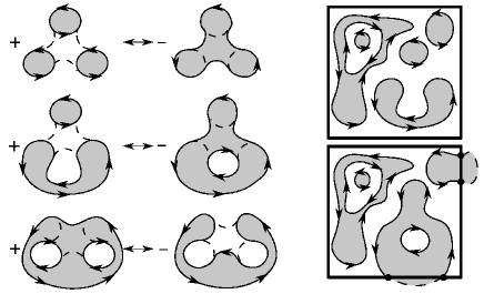
Figure 6: The three different actions of the effective Hamiltonian on the topology of loop configurations are shown in panel (a). Panels (b) and (c) show representations of two configurations by fully–packed directed loops.pollmann2006d

However, a fermionic sign problem remains: Ring–exchange processes around empty and occupied hexagons carry opposite signs in Eq. (3). We argue that it can be avoided in certain (but not all) cases. pollmann2006d In order to do so, we represent the ground–state manifold by ensembles of fully–packed loops as exemplified in Fig. 1. We notice that a ring exchange around a hexagon with an occupied center site does not change the loop topology, whereas a ring exchange around an empty hexagon always does cause changes in one of the three topological different ways shown in Fig. 6(a).

Let us consider allowed configurations with “fixed” boundary conditions with an even number of fermions on the four boundaries. They are represented by closed loops in the interior and loops terminating at a boundary. We orient the closed loops as follows: (i) Color the areas separated by the loops alternatively white and grey, with white being the outmost color; (ii) orient all loops so that the white regions are always to the right, see Fig. 6(b). If open loops are present [Fig. 6(c)], these are closed arbitrarily but intersection-free outside the sample and colored as described above. Let us assume without loss of generality that the color at infinity is white. We now notice by inspection of Fig. (6) that the relative signs resulting from the exchange processes around empty hexagons are consistent with multiplying each loop configuration by $i^{r}(-i)^{l},$ where $r$ and $l$ are the total number of the clockwise and counter–clockwise winding loops, respectively. Hence, by simultaneously changing the sign of the exchange–processes around empty hexagons and transforming the loop states

$$|\mathcal{L}\rangle \rightarrow i^{l(\mathcal{L})}(-i)^{r(\mathcal{L})}|\mathcal{L}\rangle,$$ (5)

we cure the sign problem, thus making the system effectively bosonic.

This construction need not work for periodic boundary conditions: Firstly, only even–winding subensembles (sectors) on a torus allow for such a two–color coloring. Secondly, even then it might be possible to dynamically reverse the coloring while returning to the same loop configuration. However, the exact diagonalization results presented below (see Fig. 8) suggest that for periodic boundary conditions on even tori (preserving the bipartiteness of the lattice), the lowest–energy states belong to a sector where such a transformation works. We remark that the presented non–local loop–orienting construction is restricted to the effective Hamiltonian (3), i.e., to the ring–exchange processes of length six.

V Ground states and lowest excitations in the undoped case

In order to discuss the possible confinement of fcp’s, we have to investigate the nature of the quantum–mechanical ground state of the undoped system. We do so in the approximation of an effective ring-exchange Hamiltonian (3) acting only on the subset of allowed configurations. Following Rokhsar and Kivelson, rokhsar1988 we add to $H_{\mathrm{eff}}$ an extra term that counts the number of flippable hexagons. The extended Hamiltonian reads

$$H_{\mathrm{g}\mu} = H_{\mathrm{eff}}+\mu{\textstyle\sum_{\{\psset{unit=19.91693pt}\pspicture[0.2](7.96677pt,3.98338pt)\psset{linewidth=0.5975pt,linestyle=solid}{\psset{}\pspolygon(0.0pt,1.99168pt)(1.99168pt,0.0pt)(5.97507pt,0.0pt)(7.96677pt,1.99168pt)(5.97507pt,3.98338pt)(1.99168pt,3.98338pt)}\endpspicture\;,\;\psset{unit=19.91693pt}\pspicture[0.15](3.98338pt,6.97092pt)\psset{linewidth=0.5975pt,linestyle=solid}{\psset{}\pspolygon(1.99168pt,-1.99168pt)(0.0pt,0.0pt)(0.0pt,3.98338pt)(1.99168pt,5.97507pt)(3.98338pt,3.98338pt)(3.98338pt,0.0pt)}\endpspicture\;\}}}\big{(}|\;\psset{unit=19.91693pt}\pspicture[0.2](19.91693pt,9.95847pt)\psset{linewidth=0.5975pt,linestyle=solid}{\psset{}\pspolygon(0.0pt,4.97923pt)(4.97923pt,0.0pt)(14.9377pt,0.0pt)(19.91693pt,4.97923pt)(14.9377pt,9.95847pt)(4.97923pt,9.95847pt)}\psset{linewidth=0.5975pt,linestyle=solid}{\psset{fillcolor=lightgray,fillstyle=solid}\pspolygon(4.97923pt,0.0pt)(14.9377pt,0.0pt)(9.95847pt,4.97923pt)}{\psset{fillcolor=lightgray,fillstyle=solid}\pspolygon(4.97923pt,9.95847pt)(14.9377pt,9.95847pt)(9.95847pt,4.97923pt)}{\psset{}\psline(9.95847pt,0.0pt)(9.95847pt,9.95847pt)}\psset{linewidth=1.59335pt,linestyle=solid}{\psset{linecolor=black,dotsize=2.98753pt 0.0}\psdots(4.97923pt,0.0pt)(4.97923pt,9.95847pt)(19.91693pt,4.97923pt)}{\psset{linecolor=gray,dotsize=2.98753pt 0.0}\psdots(9.95847pt,4.97923pt)}\endpspicture\;\rangle\langle\;\psset{unit=19.91693pt}\pspicture[0.2](19.91693pt,9.95847pt)\psset{linewidth=0.5975pt,linestyle=solid}{\psset{}\pspolygon(0.0pt,4.97923pt)(4.97923pt,0.0pt)(14.9377pt,0.0pt)(19.91693pt,4.97923pt)(14.9377pt,9.95847pt)(4.97923pt,9.95847pt)}\psset{linewidth=0.5975pt,linestyle=solid}{\psset{fillcolor=lightgray,fillstyle=solid}\pspolygon(4.97923pt,0.0pt)(14.9377pt,0.0pt)(9.95847pt,4.97923pt)}{\psset{fillcolor=lightgray,fillstyle=solid}\pspolygon(4.97923pt,9.95847pt)(14.9377pt,9.95847pt)(9.95847pt,4.97923pt)}{\psset{}\psline(9.95847pt,0.0pt)(9.95847pt,9.95847pt)}\psset{linewidth=1.59335pt,linestyle=solid}{\psset{linecolor=black,dotsize=2.98753pt 0.0}\psdots(4.97923pt,0.0pt)(4.97923pt,9.95847pt)(19.91693pt,4.97923pt)}{\psset{linecolor=gray,dotsize=2.98753pt 0.0}\psdots(9.95847pt,4.97923pt)}\endpspicture\;|+|\;\psset{unit=19.91693pt}\pspicture[0.2](19.91693pt,9.95847pt)\psset{linewidth=0.5975pt,linestyle=solid}{\psset{}\pspolygon(0.0pt,4.97923pt)(4.97923pt,0.0pt)(14.9377pt,0.0pt)(19.91693pt,4.97923pt)(14.9377pt,9.95847pt)(4.97923pt,9.95847pt)}\psset{linewidth=0.5975pt,linestyle=solid}{\psset{fillcolor=lightgray,fillstyle=solid}\pspolygon(4.97923pt,0.0pt)(14.9377pt,0.0pt)(9.95847pt,4.97923pt)}{\psset{fillcolor=lightgray,fillstyle=solid}\pspolygon(4.97923pt,9.95847pt)(14.9377pt,9.95847pt)(9.95847pt,4.97923pt)}{\psset{}\psline(9.95847pt,0.0pt)(9.95847pt,9.95847pt)}\psset{linewidth=1.59335pt,linestyle=solid}{\psset{linecolor=black,dotsize=2.98753pt 0.0}\psdots(0.0pt,4.97923pt)(14.9377pt,0.0pt)(14.9377pt,9.95847pt)}{\psset{linecolor=gray,dotsize=2.98753pt 0.0}\psdots(9.95847pt,4.97923pt)}\endpspicture\;\rangle\langle\;\psset{unit=19.91693pt}\pspicture[0.2](19.91693pt,9.95847pt)\psset{linewidth=0.5975pt,linestyle=solid}{\psset{}\pspolygon(0.0pt,4.97923pt)(4.97923pt,0.0pt)(14.9377pt,0.0pt)(19.91693pt,4.97923pt)(14.9377pt,9.95847pt)(4.97923pt,9.95847pt)}\psset{linewidth=0.5975pt,linestyle=solid}{\psset{fillcolor=lightgray,fillstyle=solid}\pspolygon(4.97923pt,0.0pt)(14.9377pt,0.0pt)(9.95847pt,4.97923pt)}{\psset{fillcolor=lightgray,fillstyle=solid}\pspolygon(4.97923pt,9.95847pt)(14.9377pt,9.95847pt)(9.95847pt,4.97923pt)}{\psset{}\psline(9.95847pt,0.0pt)(9.95847pt,9.95847pt)}\psset{linewidth=1.59335pt,linestyle=solid}{\psset{linecolor=black,dotsize=2.98753pt 0.0}\psdots(0.0pt,4.97923pt)(14.9377pt,0.0pt)(14.9377pt,9.95847pt)}{\psset{linecolor=gray,dotsize=2.98753pt 0.0}\psdots(9.95847pt,4.97923pt)}\endpspicture\;|\big{)},$$ (6)

where the pictographic operators with grey–colored dots in the center are summed over all flippable hexagons, independent of the occupancy of the site in the center. Next, we discuss some limiting cases of the Hamiltonian (6):

(a)

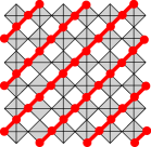
(b)

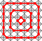
(c)

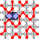
Figure 7: (a)–(b) Fragments of possible “frozen” ground states (no flippable hexagons). (c) One of several configurations of the half–filled checkerboard lattice that maximize the number of flippable hexagons. The unit cell contains $\sqrt{20}\times\sqrt{20}$ sites.

(i) $\mu\rightarrow+\infty$: All configurations which contain no flippable hexagons (frozen configurations) become ground states with $E=0$. Some are shown as Fig. 7 (a,b).
(ii) $\mu\rightarrow-\infty$: Ground states are configurations with maximal number of flippable hexagons $N_{\mathrm{fl}}$. Using a simple Metropolis–like Monte Carlo algorithm for lattices with up to 1000 sites, we always find that configurations of the type shown in Fig. 7(c) or slight variations thereof maximize $N_{\mathrm{fl}}$. Such configurations will be referred to as “squiggle” configurations.penc2006 Our numerical results suggest that in the thermodynamic limit the degenerate ground–state configurations all lie in the $(\kappa_{x},\kappa_{y})=(0,0)$ subspace.
(iii) $\mu=g>0$: This is the exactly solvable Rokhsar–Kivelson (RK) point. rokhsar1988 Following the original RK construction, we rewrite the Hamiltonian (6) for $\mu=g$ in a way which explictly shows that some liquid–like ground states have energy $E=0$ and, thus, become degenerate with the frozen states, i.e., the $\mu$$\rightarrow$$+$$\infty$ solutions. We assume that we can use the gauge transformation (5) to change the sign in the second term and to rewrite the Hamiltonian as

$$H_{\mathrm{g}=\mu} = g\sum_{\{\psset{unit=19.91693pt}\pspicture[0.2](7.96677pt,3.98338pt)\psset{linewidth=0.5975pt,linestyle=solid}{\psset{}\pspolygon(0.0pt,1.99168pt)(1.99168pt,0.0pt)(5.97507pt,0.0pt)(7.96677pt,1.99168pt)(5.97507pt,3.98338pt)(1.99168pt,3.98338pt)}\endpspicture\;,\;\psset{unit=19.91693pt}\pspicture[0.15](3.98338pt,6.97092pt)\psset{linewidth=0.5975pt,linestyle=solid}{\psset{}\pspolygon(1.99168pt,-1.99168pt)(0.0pt,0.0pt)(0.0pt,3.98338pt)(1.99168pt,5.97507pt)(3.98338pt,3.98338pt)(3.98338pt,0.0pt)}\endpspicture\;\}}\big{[}\big{(}|\!\;\psset{unit=19.91693pt}\pspicture[0.2](19.91693pt,9.95847pt)\psset{linewidth=0.5975pt,linestyle=solid}{\psset{}\pspolygon(0.0pt,4.97923pt)(4.97923pt,0.0pt)(14.9377pt,0.0pt)(19.91693pt,4.97923pt)(14.9377pt,9.95847pt)(4.97923pt,9.95847pt)}\psset{linewidth=0.5975pt,linestyle=solid}{\psset{fillcolor=lightgray,fillstyle=solid}\pspolygon(4.97923pt,0.0pt)(14.9377pt,0.0pt)(9.95847pt,4.97923pt)}{\psset{fillcolor=lightgray,fillstyle=solid}\pspolygon(4.97923pt,9.95847pt)(14.9377pt,9.95847pt)(9.95847pt,4.97923pt)}{\psset{}\psline(9.95847pt,0.0pt)(9.95847pt,9.95847pt)}\psset{linewidth=1.59335pt,linestyle=solid}{\psset{linecolor=black,dotsize=2.98753pt 0.0}\psdots(4.97923pt,0.0pt)(4.97923pt,9.95847pt)(19.91693pt,4.97923pt)}{\psset{linecolor=gray,dotsize=2.98753pt 0.0}\psdots(9.95847pt,4.97923pt)}\endpspicture\;\!\rangle-|\;\psset{unit=19.91693pt}\pspicture[0.2](19.91693pt,9.95847pt)\psset{linewidth=0.5975pt,linestyle=solid}{\psset{}\pspolygon(0.0pt,4.97923pt)(4.97923pt,0.0pt)(14.9377pt,0.0pt)(19.91693pt,4.97923pt)(14.9377pt,9.95847pt)(4.97923pt,9.95847pt)}\psset{linewidth=0.5975pt,linestyle=solid}{\psset{fillcolor=lightgray,fillstyle=solid}\pspolygon(4.97923pt,0.0pt)(14.9377pt,0.0pt)(9.95847pt,4.97923pt)}{\psset{fillcolor=lightgray,fillstyle=solid}\pspolygon(4.97923pt,9.95847pt)(14.9377pt,9.95847pt)(9.95847pt,4.97923pt)}{\psset{}\psline(9.95847pt,0.0pt)(9.95847pt,9.95847pt)}\psset{linewidth=1.59335pt,linestyle=solid}{\psset{linecolor=black,dotsize=2.98753pt 0.0}\psdots(0.0pt,4.97923pt)(14.9377pt,0.0pt)(14.9377pt,9.95847pt)}{\psset{linecolor=gray,dotsize=2.98753pt 0.0}\psdots(9.95847pt,4.97923pt)}\endpspicture\;\!\rangle\big{)}\times\big{(}\langle\!\;\psset{unit=19.91693pt}\pspicture[0.2](19.91693pt,9.95847pt)\psset{linewidth=0.5975pt,linestyle=solid}{\psset{}\pspolygon(0.0pt,4.97923pt)(4.97923pt,0.0pt)(14.9377pt,0.0pt)(19.91693pt,4.97923pt)(14.9377pt,9.95847pt)(4.97923pt,9.95847pt)}\psset{linewidth=0.5975pt,linestyle=solid}{\psset{fillcolor=lightgray,fillstyle=solid}\pspolygon(4.97923pt,0.0pt)(14.9377pt,0.0pt)(9.95847pt,4.97923pt)}{\psset{fillcolor=lightgray,fillstyle=solid}\pspolygon(4.97923pt,9.95847pt)(14.9377pt,9.95847pt)(9.95847pt,4.97923pt)}{\psset{}\psline(9.95847pt,0.0pt)(9.95847pt,9.95847pt)}\psset{linewidth=1.59335pt,linestyle=solid}{\psset{linecolor=black,dotsize=2.98753pt 0.0}\psdots(4.97923pt,0.0pt)(4.97923pt,9.95847pt)(19.91693pt,4.97923pt)}{\psset{linecolor=gray,dotsize=2.98753pt 0.0}\psdots(9.95847pt,4.97923pt)}\endpspicture\;|-\langle\;\psset{unit=19.91693pt}\pspicture[0.2](19.91693pt,9.95847pt)\psset{linewidth=0.5975pt,linestyle=solid}{\psset{}\pspolygon(0.0pt,4.97923pt)(4.97923pt,0.0pt)(14.9377pt,0.0pt)(19.91693pt,4.97923pt)(14.9377pt,9.95847pt)(4.97923pt,9.95847pt)}\psset{linewidth=0.5975pt,linestyle=solid}{\psset{fillcolor=lightgray,fillstyle=solid}\pspolygon(4.97923pt,0.0pt)(14.9377pt,0.0pt)(9.95847pt,4.97923pt)}{\psset{fillcolor=lightgray,fillstyle=solid}\pspolygon(4.97923pt,9.95847pt)(14.9377pt,9.95847pt)(9.95847pt,4.97923pt)}{\psset{}\psline(9.95847pt,0.0pt)(9.95847pt,9.95847pt)}\psset{linewidth=1.59335pt,linestyle=solid}{\psset{linecolor=black,dotsize=2.98753pt 0.0}\psdots(0.0pt,4.97923pt)(14.9377pt,0.0pt)(14.9377pt,9.95847pt)}{\psset{linecolor=gray,dotsize=2.98753pt 0.0}\psdots(9.95847pt,4.97923pt)}\endpspicture\;\!|\big{)}\big{]}.$$ (7)

Since this is a sum over projectors, all eigenvalues are non–negative. Furthermore, after re–gauging, all off–diagonal elements are non–positive and for each subensemble $\ell$ an exact ground–state wavefunction is given by the equally weighted superposition of its configurations $|C_{i}^{(l)}\rangle$, i.e., $|\psi_{0,RK}^{(l)}\rangle\sim\sum_{i}|C_{i}^{(l)}\rangle$. These coherent superpositions are the analogs of the Resonating Valence Bond (RVB) state, originally discussed by L. Paulingpauling1953 and P. W. Anderson.anderson1973 Their energy is easily computed: Each flippable hexagon contributes $-g$ and $+\mu$, thus for $g=\mu$: $\langle\psi_{0,RK}^{(l)}|H_{\mathrm{g}\mu}|\psi_{0,RK}^{(l)}\rangle=0.$ Note that for fermionic systems, we find a well defined RK point only if a gauge transformation exists such that all off–diagonal matrix elements are non–positive. Otherwise the energy is most likely larger than zero and the subensembles consequently do not form a ground state.

Next, we explore by means of numerically exact diagonalization the eigenstates of small clusters general $\mu$ values. For the actual calculations, we first generate all configurations that fulfill the tetrahedron rule, then group them according to quantum numbers and generate a sparse block–diagonal matrix representation of the Hamiltonian (6). For a 72–site checkerboard cluster with periodic boundary conditions, the $16\ 448\ 400$ dimensional low–energy Hilbert space of allowed configurations can be decomposed into a few hundred subspaces, where the largest one has $1\ 211\ 016$ dimensions. The low–energy states of the sparse block–diagonal Hamiltonian matrix and physical properties such as charge density distribution and density–density correlations can easily be obtained on a 64–bit workstation. Figure 8(a) shows energies of the ground-state and the lowest excited states of all subensembles.

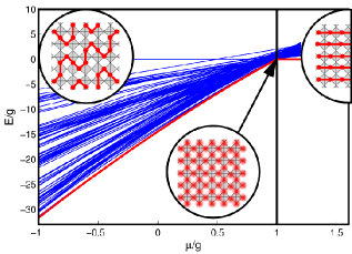
(a)  (b)

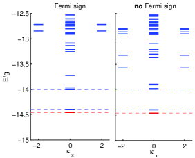
Figure 8: (a) Energies of the ground state and lowest excited states in each subensemble of a 72–site half–filled checkerboard cluster for different values of $\mu$ of the $g$–$\mu$ Hamiltonian. Level crossing of ground states occurs only at $\mu=g$. The insets indicate different phases: Maximal flippable plus fluctuations for $\mu<g$, a critical point $\mu=g$ where the ground state is an equally weighted superposition of all configurations, and frozen configurations as ground states for $\mu>g$. (b) Left side: Ground–state energy and energies of the lowest excited states of the effective Hamiltonian $H_{\mathrm{eff}}$ in subspaces with different global slopes $\left(\kappa_{x},\kappa_{y}\right)$ $=\left(\kappa_{x},0\right)$ for 72–site cluster. Right side: Same system, but assuming same signs for all matrix elements (“bosonic calculation”).pollmann2006d

(iv) For $\mu<g$, two ground states are found in subensembles with $(\kappa_{x},\kappa_{y})=(0,0)$ and $(N_{\mathcal{B}},N_{\mathcal{Y}},N_{\mathcal{G}},N_{\mathcal{R}})=(6,6,12,12)$ and $(12,12,6,6)$, respectively. These are superpositions of configurations with the maximal number of flippable hexagons. At the physical point $\mu=0$, the 72–site system is in a crystalline and confining phase. In the thermodynamic limit, we expect to recover the 10–fold degeneracy of the squiggle phase instead of the two–fold degeneracy. For small values $\mu>0$, the average weight of configurations in the ground state with the maximum number $N_{\mathrm{fl}}$ is large (not shown), but decreases with increasing $\mu$ until at the RK point, i.e., $\mu$=$g$, the ground state is formed by an equally weighted superposition of all configurations of a certain subensemble.

(v) For $\mu>g$, we find essentially the same properties as described above in the limit $\mu\rightarrow\infty.$

In summary, we find a confining phase and a phase in which the ground states are given by static isolated configurations. The two phases are separated by a point with deconfined excitations, i.e., the Rokhsar–Kivelson (RK) point. rokhsar1988 The main finding is that the original effective Hamiltonian is in a confining phase with a long–range ordered ground state (squiggle phase). This phase maximizes the gain in kinetic energy and is stabilized by quantum fluctuations (order from disorder). The results of the exact diagonalization on small samples indicate that the symmetry remains broken all the way along the $\mu$–axis up to the RK point. This observation is also strongly disfavoring a deconfining phase to the left of the RK point. Hence, the fermionic RK point is likely to be an isolated quantum critical point just as it is for the bosonic model.shannon2004

We come back to the fermionic sign problem. Figure 8(b) compares energies of a system in which the Fermi sign is taken into account to those from calculations which exclude the Fermi sign. The ground–state energy, the first excited states in the $(\kappa_{x},\kappa_{y})=(0,0)$ sector, and the weights of the different configurations in the corresponding eigenstates are the same in both case. In some subensembles with $(\kappa_{x},\kappa_{y})\neq(0,0)$ the energies of the ground states including the Fermi sign are higher than the ones for bosons (no Fermi sign).

(a)

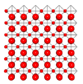
(b)

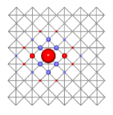
(c)

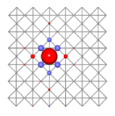
Figure 9: Half filling: (a) Charge density distribution for one of the two ground sates. (b) Corresponding density–density correlation function $C_{i_{0}i}^{(l)}$. The site $i_{0}$ with average density 2/3 shows up as the largest dot in the panels (b)–(c). The radius of the dots is proportional to the absolute value. A red or blue color represents a positive or negative value, respectively. (c) Classical density–density correlation function.

At the physical point $\mu=0,$ the 72–site ground state is two-fold degenerate with quantum numbers $(N_{\mathcal{B}},N_{\mathcal{Y}},N_{\mathcal{G}},N_{\mathcal{R}})=(6,6,12,12)$ or $(12,12,6,6)$. The resulting charge order with alternating stripes of average occupation $1/3$ and $2/3$ is shown in Fig. 9(a). The density–density correlation function in the quantum–mechanical ground states $|\psi_{0}^{(l)}\rangle$ [Fig. 9(b)]

$$C_{i_{0}i}^{(l)}=\langle\psi_{0}^{(l)}|n_{i}n_{i_{0}}|\psi_{0}^{(l)}\rangle-\langle\psi_{0}^{(l)}|n_{i}|\psi_{0}^{(l)}\rangle\langle\psi_{0}^{(l)}|n_{i0}|\psi_{0}^{(l)}\rangle.$$ (8)

is best understood as reflecting the algebraic correlations present in the average over all classically degenerate configurations, see Fig. 9(c) and Ref. pollmann2006a . Specific quantum–mechanical features resulting from ring hopping become visible in the difference of the actual correlations and have been discussed in Ref. runge2004 .

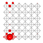
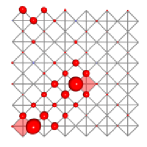
(a)	(b)	(e)
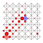
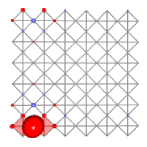
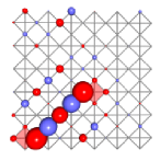
(c)	(d)	(f)

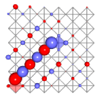
Figure 10: (a), (b), and (e): Local loss of kinetic energy due to the separation of two fractionally (static) charged defects (fcp’s marked by light red squares or fch’s marked by dark blue squares). The radii of the circles are proportional to the local energy loss. (c), (d), and (f): Red (blue) circles show an increase (decrease) of the local density (vacuum polarization due to the two fcp’s or the fcp–fch pair).

VI Static and dynamical properties of the doped system

Next, we turn to the important issue of confinement/deconfinement of defects generated either particle–hole excitations or by weak doping. Two different kinds of calculations can be done: In the first case—referred to as static charges—the defects are fixed to some lattice positions and ground–state calculations involving $H_{\mathrm{eff}}$ are performed in the restricted subspace spanned by the configurations with exactly those defects at given positions. The total (free) energy is recorded as function of the defect positions. Its spatial derivative is interpreted as attractive or repulsive force. In the second case—referred to as dynamic charges—the defects propagate according to the Hamiltonian (4). The existence or non–existence of bound states is interpreted as confinement or deconfinement.

Static charges.

If an additional particle is added/doped to a half-filled checkerboard lattice, at least two crisscrossed squares are occupied by three particles. It is easy to see that, e.g., for the $t$–$\mu$ Hamiltonian in the limit of large positive $\mu$ (frozen configurations) the ground–state energy of two static fractional charges is independent of the distance between. Thus static charges are not attracted by a force, which suggests that dynamic fcp’s are deconfined at zero temperature in that limit.

Also, it is obvious that at the RK point the total energy of a system with two static charges is independent of the distance between them. Thus dynamic fcp’s are expected to be deconfined.

We will not discuss systems with a general values of $\mu$ further, but focus on the physical case $\mu=0$ and discuss the changes of the kinetic energy density in the presence of two static charges $e/2$.pollmann2006c The energy change can be decomposed into local contributions $\epsilon_{i}$ from all ring–exchange processes involving a given site $i$. An increase in kinetic energy in the region between the two fractional charges, i.e., along the connecting string, is found and illustrated in Fig. 10(a,b). The total energy increase is approximately proportional to the length of the generated string and implies at large distances a constant confining force. The changes of the local energy density goes along with density changes, as illustrated in Fig. 10(c,d). Similar results are found when a particle is removed from the ground state or when a particle–hole excitation is generated out of the ground state, see Fig. 10(c,d,f).

The calculations have been performed in a reduced Hilbert space in which only two static defects are present. In a calculation within the full Hilbert space, or a subspace allowing at least an additional fcp–fch pair, the energy would not increase linearly to infinity, but the connecting string is expected to break by creating additional pairs of defects when this energetically favorable. For the relevant parameters, e.g., $g=0.01t$ and $V=10t$, this occurs when two fcp’s have separated over 1000 lattice sites. This effect is well known for the case of confined quarks where pair production (quark anti–quark pairs) occurs before the quarks have been separated to an observable distance.

The attractive constant force acting between two fractional charges in the confining phase results from a reduction of vacuum fluctuations and a polarization of the vacuum in the vicinity of the connecting strings. These findings suggest that a number of features known from QCD are also expected to occur in a modified form in solid–state physics. Conversely, one would hope that by studying frustrated lattices or dimer models one might be able to obtain better insight into certain aspects of QCD.

Dynamic charges.

We turn now to the dynamical properties of fcp’s, in particular spectral functions and optical conductivity for the half–filled checkerboard lattice. Numerical studies of finite clusters are again the method of choice,pollmann2006d because conventional approximation schemes such as mean–field theories or Green’s function decoupling schemes are unable to describe the strong local correlations expressed by the tetrahedron rule. Diagonalizations with up to 50 sites were performed within the minimal Hilbert space spanned by the configurations with the smallest possible number of violations of the tetrahedron rule [half–filled system: all allowed configurations plus those with one fcp–fch pair; doped case: 2 fcp’s or 2 fch’s].

The spectral function $A(\mathbf{k},\omega)=A^{-}(\mathbf{k},\omega)+A^{+}(\mathbf{k},\omega)$ of an interacting many–particle system is the sum of the probability amplitudes for adding (+) to the $N$–particle ground–state system $|\psi_{0}^{N}\rangle$ or removing (–) from it a particle with momentum $\mathbf{k}$ and energy $\omega$ ($\hbar=1$)

$$A^{+}(\mathbf{k},\omega) = \lim_{\eta\rightarrow 0^{+}}-\frac{1}{\pi}\mbox{Im}\langle\psi_{0}^{N}|c_{\mathbf{k}}\ \frac{1}{\omega+i\eta+E_{0}-H}\ c_{\mathbf{k}}^{{\dagger}}|\psi_{0}^{N}\rangle$$ (9)

$$A^{-}(\mathbf{k},\omega) = \lim_{\eta\rightarrow 0^{+}}-\frac{1}{\pi}\mbox{Im}\langle\psi_{0}^{N}|\ c_{\mathbf{k}}^{{\dagger}}\ \frac{1}{\omega+i\eta-E_{0}+H}\ c_{\mathbf{k}}|\psi_{0}^{N}\rangle.$$ (10)

We use operators $c_{\mathbf{k}}^{{\dagger}}=\frac{1}{\sqrt{N}}\sum_{j}e^{i\mathbf{r}_{j}\mathbf{k}}c_{j}^{{\dagger}}$ in the extended Brillouin zone.

The spectral functions yield direct insight into the dynamics of a many–body system, as seen, e.g., in angular–resolved photoemission spectroscopy (ARPES). Expectation values of the form $G(z)=\langle\psi_{0}|A\ \,(z-H)^{-1}\ A^{{\dagger}}|\psi_{0}\rangle$ can conveniently be calculated numerically by the Lanczos continued fraction method gagliano1987 or kernel polynomial expansion silver1996 . We found essentially identical results for both algorithms.pollmannDissertation However, the implementation of the Lanczos method turned out to be slightly faster. Well converged results were obtained already after several hundred iterations.

(a)

(b)

(a) Spectral function $A(\mathbf{k}=\pi/2,\omega)$ for $V=25t$ calculated for a $\sqrt{32}\times\sqrt{32}$ cluster for the effective $t$–$g$ Hamiltonian with (a) $g=0.01$ and (b) $g=1$. A Lorentzian broadening $\eta=0.1t$ is used.

We checked numerically that in the limit of large $V$, it is sufficient to calculate the spectral functions within the minimal Hilbert space. This enables us to study rather large systems and to address the question whether or not the two defects created by injecting one particle are closely bound to one another or not.

The concept of a spatial separation of fcp’s can be confirmed by comparing results within the minimal Hilbert space with those from an artificially restricted calculation in which a particle is prevented from decaying into two defects with charge $e/2$ each. In our finite–cluster calculations, a broad low–energy continuum is seen in the spectral functions for the unrestricted case, which is missing when the restriction is imposed.pollmann2006c The respective bandwidths are about $13t$ and $8t$. This suggests a simple interpretation: The dynamics of two separated fcp’s having a bandwidth of $\approx 6t$ each due to six nearest neighbors would explain the calculated $13t$, while a confined added particle has a much smaller bandwidth $8t$, which is close to $6t$.

Further insight can be obtained if the amplitude of the ring exchange $g$=$12t^{3}/V^{2}$ in the effective Hamiltonian is considered an independent parameter which is no longer restricted to the regime $g$$\ll$$t$ as enforced by $t$$\ll$$V$. Figure VI compares results for the “physical” regime corresponding to the previously considered parameters $g\sim t^{3}/V^{2}=0.01t$ with those for $g=t$. In the latter case, the broad continuum at the bottom of the spectral density vanishes and a sharp $\delta$–peak evolves instead. The latter should be viewed as a Landau quasi-particle peak. This suggests the following interpretation: The ring exchange term leads for the undoped case to charge order, which in finite–cluster calculations is destroyed when a particle is added by the separation of the two fcp’s. These are weakly bound to each other. If $g$$\ll$$t$, the distance of the two fcp’s is larger than the system size considered and thus the excitations seem to be deconfined. An artificially increased $g$ leads to much stronger confinement and the diameter of the bounded pair becomes smaller or comparable to the system size. The pair acts at low energies as one entity. The electron as a (however strongly modified) “particle” is recovered and a finite weight of the quasi-particle peak results. These findings suggest that for the physical regime $V/t\approx 10$ quasi-particles with a spatial extent over more than hundred lattice sites are formed. The huge spatial extent is expected to lead to interesting effect. E.g., one may find with increasing doping concentration a transition from a “confined” phase to an “fcp plasma” phase with yet unknown properties when the average distance of bound fcp–fcp pairs falls below the diameter of a single bound fcp pair. Other open questions for future research include a thorough investigation of the 3D pyrochlore lattice. Even though the checkerboard lattice and pyrochlore lattice show many similarities, there exist certain differences between them, e.g., due to the higher spatial dimensionality.hermele2004 ; pollmann2006e Here, differences of the two lattices arise in the U(1) gauge theory which describes the low energy excitations of the considered systems. The related compact electrodynamic is always confining in 2+1 dimensions while it allows for the existence of a deconfined phase in 3+1 dimension.polyakov1977 Systematic exact diagonalization studies as well as the application of Monte Carlo techniques will provide a deeper insight and we hope to confirm the expected existence of a deconfined phase in a 3D pyrochlore lattice. In addition, a natural extension of the model considered in this paper is the inclusion of spin. This leads to a more realistic model and could provide a better link to experiments.

References

- (1) W. P. Su, J. R. Schrieffer and A. J. Heeger, Phys. Rev. Lett. 42, p. 1698 (1979).
- (2) R. B. Laughlin, Phys. Rev. Lett. 50, p. 1395 (1983).
- (3) P. Fulde, K. Penc and N. Shannon, Ann. Phys. (Leipzig) 11, p. 893 (2002).
- (4) S. Kondo, D. C. Johnston, C. A. Swenson, F. Borsa, A. V. Mahajan, L. L. Miller, T. Gu, A. I. Goldman, M. B. Maple, D. A. Gajewski, E. J. Freeman, N. R. Dilley, R. P. Dickey, J. Merrin, K. Kojima, G. M. Luke, Y. J. Uemura, O. Chmaissem and J. D. Jorgensen, Phys. Rev. Lett. 78, p. 3729 (1997).
- (5) W. Hofstetter, J. I. Chirac, P. Zoller, E. Demler and M. D. Lukin, Phys. Rev. Lett. 89, p. 220407 (2002).
- (6) G. Misguich and C. Lhuillier, cond-mat/0310405 (October 2003), in Ref. diep2005 , p. 229ff.
- (7) H. T. Diep (ed.), Frustrated Spin Systems (World Scientific, Singapore, 2005).
- (8) M. Hermele, M. P. A. Fisher and L. Balents, Phys. Rev. B 69, p. 064404 (2004).
- (9) A. Läuchli and D. Poilblanc, Phys. Rev. Lett. 92, p. 236404 (2004).
- (10) N. Shannon, G. Misguich and K. Penc, Phys. Rev. B 69, p. 220403(R) (2004).
- (11) R. Moessner, O. Tchernyshyov and S. L. Sondhi, J. Stat. Phys. 116, p. 755 (2004).
- (12) P. W. Anderson, Phys. Rev. 102, p. 1008 (1956).
- (13) E. Runge and P. Fulde, Phys. Rev. B 70, p. 245113 (2004).
- (14) R. Baxter, Exactly Solved Models in Statistical Mechanics (Academic Press, San Diego, 1982).
- (15) F. Pollmann, J. J. Betouras and E. Runge, Phys. Rev. B 73, p. 174417 (2006).
- (16) F. Pollmann, Charge Degrees of Freedom on Frustrated Lattices, Doctoral Dissertation, Technische Universität Ilmenau, (Ilmenau, Germany, 2006), http: //nbn-resolving.de/urn/resolver.pl?urn=nbn:de:gbv:ilm1-2006000140.
- (17) F. Pollmann, J. Betouras, K. Shtengel and P. Fulde, Phys. Rev. Lett. 97, p. 170407 (2006).
- (18) D. S. Rokhsar and A. A. Kivelson, Phys. Rev. Lett. 61, p. 2376 (1988).
- (19) K. Penc and N. Shannon, private communication and to be published (2006).
- (20) L. Pauling, Proc. Natl. Acad. Sci. 39, p. 551 (1953).
- (21) P. W. Anderson, Mater. Res. Bull. 8, p. 173 (1973).
- (22) F. Pollmann, E. Runge and P. Fulde, Phys. Rev. B 73, p. 125121 (2006).
- (23) E. R. Gagliano and C. A. Balseiro, Phys. Rev. Lett. 59, p. 2999 (1987).
- (24) R. N. Silver, H. Roeder, A. F. Voter and J. D. Kress, J. Comp. Phys. 124, p. 115 (1996).
- (25) F. Pollmann, J. J. Betouras, E. Runge and P. Fulde, Charge degrees in the quarter-filled checkerboard lattice, in Proceedings of ICM2006 (Kyoto, Aug. 20-25, 2006), (in print).
- (26) A. M. Polyakov, Nucl. Phys. B 120, p. 429 (1977).