Etched Glass Surfaces, Atomic Force Microscopy and Stochastic Analysis

Abstract

The effect of etching time scale of glass surface on its statistical properties has been studied using atomic force microscopy technique. We have characterized the complexity of the height fluctuation of a etched surface by the stochastic parameters such as intermittency exponents, roughness, roughness exponents, drift and diffusion coefficients and find their variations in terms of the etching time.

I Introduction

The complexity of rough surfaces is subject of a large variety of investigations in different fields of science Barabasi ; Davies . Surface roughness has an enormous influence on many important physical phenomena such as contact mechanics, sealing, adhesion, friction and self-cleaning paints and glass windows, Bo ; Zhao . A surface roughness of just a few nanometers is enough to remove the adhesion between clean and (elastically) hard solid surfaces Bo . The physical and chemical properties of surfaces and interfaces are to a significant degree determined by their topographic structure. The technology of micro fabrication of glass is getting more and more important because glass substrates are currently being used to fabricate micro electro mechanical system (MEMS) devices Won . Glass has many advantages as a material for MEMS applications, such as good mechanical and optical properties. It is a high electrical insulator, and it can be easily bonded to silicon substrates at temperatures lower than the temperature needed for fusion bonding Melvin . Also micro and nano-structuring of glass surfaces is important for the production of many components and systems such as gratings, diffractive optical elements, planar wave guide devices, micro-fluidic channels and substrates for (bio) chemical applications Cheng . Wet etching is also well developed for some of these applications Knotter ; Spierings ; Schuitema ; Glebov ; Jafari1 ; Silikas ; Irajizad .

One of the main problems in the rough surface is the scaling behavior of the moments of height $h$ and evolution of the probability density function (PDF) of $h$, i.e. $P(h,x)$ in terms of the length scale $x$. Recently some authors have been able to obtain a Fokker-Planck equation describing the evolution of the probability distribution function in terms of the length scale, by analyzing some stochastic phenomena, such as rough surfaces Jafari2 ; Waechter ; Sangpour , turbulent system Renner , financial data Renner2 , cosmic background radiation Ghasemi and heart interbeats pei04 etc. They noticed that the conditional probability density of field increment satisfies the Chapman-Kolmogorov equation. Mathematically, this is a necessary condition for the fluctuating data to be a Markovian process in the length (time) scales Risken .

In this work, we investigate the etching process as a stochastic process. We measure the intermittency exponents of height structure function, roughness, roughness exponents and Kramers-Moyal‘s (KM) coefficients. Indeed we consider the etching time $t$, as an external parameter, to control the statistical properties of a rough surface and find their variations with $t$. It is shown that the first and second KM‘s coefficients have well-defined values, while the third and fourth order coefficients tend to zero. The first and second KM‘s coefficients for the fluctuations of $h(x)$, enables us to explain the height fluctuation of the etched glass surface.

II Experimental

We started with glass microscope slides as a sample. Only one side of samples was etched by HF solution for different etching time (less than 20 minutes). HF concentration was $\%40$ for all the experiments. The surface topography of the etched glass samples in the scale ($<5\mu m$) was obtained using an AFM (Park Scientific Instruments). The images in this scale were collected in a constant force mode and digitized into $256$$\times$$256$ pixels. A commercial standard pyramidal $Si_{3}N_{4}$ tip was used. A variety of scans, each with size $L$, were recorded at random locations on the surface. Figure 1 shows typical AFM image with resolutions of about $20nm$.

III Statistical quantities

III.1 Multifractal Analysis and the Intermittency Exponent

Assuming statistical translational invariance, the structure functions $S^{q}(l)=<|h(x+l)-h(x)|^{q}>$, (moments of the increment of the rough surface height fluctuation $h(x)$) will depend only on the space deference of heights $l$, and has a power law behavior if the process has the scaling property:

$$S^{q}(l)=<|h(x+l)-h(x)|^{q}>\propto S^{q}(L_{0})(\frac{l}{L_{0}})^{\xi(q)}$$ (1)

where $L_{0}$ is the fixed largest length scale of the system, $<\cdot\cdot\cdot>$ denotes statistical average (for non-overlapping increments of length $l$), $q$ is the order of the moment (we take here $q>0$), and $\xi(q)$ is the exponents of structure function. The second moment is linked to the slope $\beta$ of the Fourier power spectrum: $\beta=1+\xi_{2}$. The main property of a multifractal processes is that it is characterized by a non-linear $\xi_{q}$ function verses $q$. Monofractals are the generic result of this linear behavior. For instance, for Brownian motion (Bm) $\xi_{q}=q/2$, and for fractional Brownian motion (fBm) $\xi_{q}\propto q$.

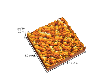
Figure 1: AFM surface image of etched glass film with size $5\times 5\mu m^{2}$ after 12 minutes.

III.2 Roughness and Roughness Exponents

It is also known that to derive the quantitative information of the surface morphology one may consider a sample of size $L$ and define the mean height of growing film $\overline{h}$ and its variance, $\sigma$ by:

$$\sigma(L,t)=(\langle(h-\overline{h})^{2}\rangle)^{1/2}$$ (2)

where $t$ is etching time and $\langle\cdots\rangle$ denotes an averaging over different samples, respectively. Moreover, etching time is a factor which can apply to control the surface roughness of thin films.

Let us now calculate also the roughness exponent of the etched glass. Starting from a flat interface (one of the possible initial conditions), it is conjectured that a scaling of space by factor $b$ and of time by factor $b^{z}$ ($z$ is the dynamical scaling exponent), rescales the variance, $\sigma$ by factor $b^{\chi}$ as follows Barabasi :

$$\sigma(bL,b^{z}t)=b^{\alpha}\sigma(L,t)$$ (3)

which implies that

$$\sigma(L,t)=L^{\alpha}f(t/L^{z}).$$ (4)

If for large $t$ and fixed $L$ $(x=t/L^{z}\rightarrow\infty)$ $\sigma$ saturate. However, for fixed large $L$ and $t\ll L^{z}$, one expects that correlations of the height fluctuations are set up only within a distance $t^{1/z}$ and thus must be independent of $L$. This implies that for $x\ll 1$, $f(x)\sim x^{\beta}$ with $\beta=\alpha/z$. Thus dynamic scaling postulates that

$$\sigma(L,t)\propto\left\{\begin{array}[]{ll}t^{\beta},&\hbox{t$\ll L^{z}$;}\\ L^{\alpha},&\hbox{t$\gg L^{z}$}.\\ \end{array}\right.$$ (7)

The roughness exponent $\alpha$ and the dynamic exponent $\beta$ characterize the self-affine geometry of the surface and its dynamics, respectively.

The common procedure to measure the roughness exponent of a rough surface is use of the surface structure function depending on the length scale $l$ which is defined as:

$$S^{2}(l)=\langle|h(x+l)-h(x)|^{2}\rangle.$$ (8)

It is equivalent to the statistics of height-height correlation function $C(l)$ for stationary surfaces, i.e. $S^{2}(l)=2\sigma^{2}(1-C(l))$. The second order structure function $S(l)$, scales with $l$ as $l^{2\alpha}$ Barabasi .

III.3 The Markov Nature of Height Fluctuations: Drift and Diffusion Coefficients

We check whether the data of height fluctuations follow a Markov chain and, if so, measure the Markov length scale $l_{M}$. As is well-known, a given process with a degree of randomness or stochasticity may have a finite or an infinite Markov length scale Markov . The Markov length scale is the minimum length interval over which the data can be considered as a Markov process. To determine the Markov length scale $l_{M}$, we note that a complete characterization of the statistical properties of random fluctuations of a quantity $h$ in terms of a parameter $x$ requires evaluation of the joint PDF, i.e. $P_{N}(h_{1},x_{1};....;h_{N},x_{N})$, for any arbitrary $N$. If the process is a Markov process (a process without memory), an important simplification arises. For this type of process, $P_{N}$ can be generated by a product of the conditional probabilities $P(h_{i+1},x_{i+1}|h_{i},x_{i})$, for $i=1,...,N-1$. As a necessary condition for being a Markov process, the Chapman-Kolmogorov equation,

$$P(h_{2},x_{2}|h_{1},x_{1})=$$ (9)

$$\int\hbox{d}(h_{i})\,P(h_{2},x_{2}|h_{i},x_{i})\,P(h_{i},x_{i}|h_{1},x_{1})$$ (10)

should hold for any value of $x_{i}$, in the interval $x_{2}<x_{i}<x_{1}$ Risken .

The simplest way to determine $l_{M}$ for homogeneous surface is the numerical calculation of the quantity, $S=|P(h_{2},x_{2}|h_{1},x_{1})-\int\hbox{d}h_{3}P(h_{2},x_{2}|h_{3},x_{3})\,P(h_{3},x_{3}|h_{1},x_{1})|$, for given $h_{1}$ and $h_{2}$, in terms of, for example, $x_{3}-x_{1}$ and considering the possible errors in estimating $S$. Then, $l_{M}=x_{3}-x_{1}$ for that value of $x_{3}-x_{1}$ such that, $S=0$ Markov .

It is well-known, the Chapman-Kolmogorov equation yields an evolution equation for the change of the distribution function $P(h,x)$ across the scales $x$. The Chapman-Kolmogorov equation formulated in differential form yields a master equation, which can take the form of a Fokker-Planck equation Risken ; Markov :

$$\frac{\partial}{\partial x}P(h,x)=[-\frac{\partial}{\partial h}D^{(1)}(h,x)+\frac{\partial^{2}}{\partial h^{2}}D^{(2)}(h,x)]P(h,x).$$ (11)

The drift and diffusion coefficients $D^{(1)}(h,r)$, $D^{(2)}(h,r)$ can be estimated directly from the data and the moments $M^{(k)}$ of the conditional probability distributions:

$$D^{(k)}(h,x)=\frac{1}{k!}{\rm lim}_{r\rightarrow 0}M^{(k)}$$ (12)

$$M^{(k)}=\frac{1}{r}\int dh^{\prime}(h^{\prime}-h)^{k}P(h^{\prime},x+r|h,x).$$ (13)

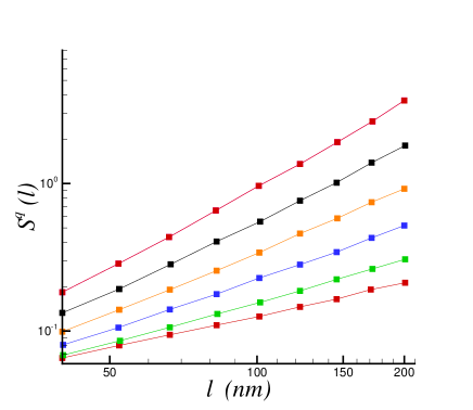
Figure 2: Scaling of the structure functions in log-log plot for moments less than 8. (from bottom to top).

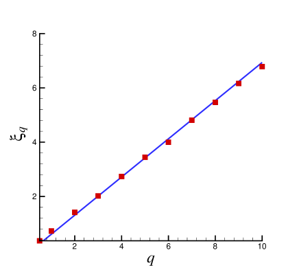
Figure 3: The results of scaling exponent $\xi_{q}$ which is clearly linear vs. q.

The coefficients $D^{(k)}(h,x)$‘s are known as Kramers-Moyal coefficients. According to Pawula‘s theorem Risken , the Kramers-Moyal expansion stops after the second term, provided that the fourth order coefficient $D^{(4)}(h,x)$ vanishes Risken . The forth order coefficients $D^{(4)}$ in our analysis was found to be about ${D^{(4)}}\simeq 10^{-4}{D^{(2)}}$. In this approximation, we can ignore the coefficients $D^{(n)}$ for $n\geq 3$. We note that this Fokker-Planck equation is equivalent to the following Langevin equation (using the Ito interpretation) Risken :

$$\frac{\partial}{\partial x}h(x)=D^{(1)}(h,x)+\sqrt{D^{(2)}(h,x)}f(x)$$ (14)

where $f(x)$ is a random force, zero mean with gaussian statistics, $\delta$-correlated in $x$, i.e. $\langle f(x)f(x^{\prime})\rangle=2\delta(x-x^{\prime})$. Furthermore, with this last expression, it becomes clear that we are able to separate the deterministic and the noisy components of the surface height fluctuations in terms of the coefficients $D^{(1)}$ and $D^{(2)}$.

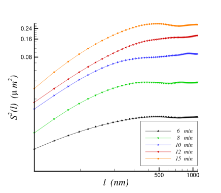
Figure 4: Log-Log plot of selection structure function of the etched glass surfaces.

IV Results and Discussion

Now, using the introduced statistical parameters in the previous sections, it is possible to obtain some quantitative information about the effect of etching time on surface topography of the glass surface. To study the effect of the etching time on the surface statistical characteristics, we have utilized AFM imaging technique in order to obtain microstructural data of the etched glass surfaces at the different etching time in the HF. Figure 1 shows the AFM image of etched glass after $12$ minuets etched. To investigate the scaling behavior of the moments of $\delta h_{l}=h(x+l)-h(x)$, we consider the samples that they reached to the stationary state. This means that their statistical properties do not change with time. In our case the samples with etching time more than $20$ minutes are almost stationary. Figure 2 shows the log-log plot of the structure functions verses length scale $l$ for different orders of moments. The straight lines show that the moments of order $q$ have the scaling behavior. We have checked the scaling relation up to moment $q=10$. The resulting intermittency exponent $\xi_{q}$ is shown in figure 3. It is evident that $\xi_{q}$ has a linear behavior. This means that the height fluctuations are mono-fractal behavior. We also directly estimated the scaling exponent of the linear term $l^{qH}/<(h(x+l)-h(x))^{q}>$ and obtain the following values for the samples with 20 minuets etching time, $\xi_{1}=0.70\pm 0.04$ and $\xi_{2}=1.40\pm 0.04$. This means etching memorize fractal feature during etching. Therefore using the scaling exponent $\xi_{2}$ we obtain the roughness exponent $\alpha$ as $\xi_{2}/2=0.70\pm 0.04$.

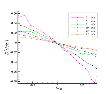
Figure 5: Drift coefficients of the surfaces at different etching time less than 20 minutes.

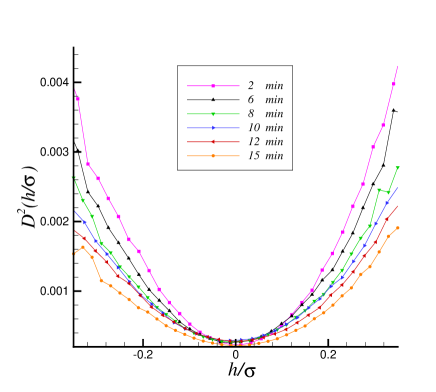
Figure 6: Diffused coefficients of the surface at different etching time less than 20 minutes.

Figure 4 presents the structure function $S(l)$ of the surface at the different etching time, using equation (8). It is also possible to evaluate the grain size dependence to the etching time, using the correlation length achieved by the structure function represented in figure 4. The correlation lengths increase with etching time. Its value has a exponential behavior $448(1-\exp(-0.15t))nm$. Also we find that the dynamical exponent is given by $\beta=0.6\pm 0.1$. Also we measured the variation of the Markov length with etching time $t$ (min), and obtain $l_{M}=40+3t$ (nm) for time scales $t<20~{}min$.

Finally to obtain the stochastic equation of the height fluctuations behavior of the surface, we need to measure the Keramer- Moyal Coefficients. In our analysis the forth order coefficients $D^{(4)}$ is less than Second order coefficients, $D^{(2)}$, about ${D^{(4)}}\simeq 10^{-4}{D^{(2)}}$. In this approximation, we ignore the coefficients $D^{(n)}$ for $n\geq 3$. So, to discuss the surfaces it just needs to measure the drift coefficient $D^{(1)}(\frac{h}{\sigma})$ and diffusion coefficient $D^{(2)}(\frac{h}{\sigma})$ using Eq. (12). Figures 5 and 6 show the drift coefficient $D^{(1)}(\frac{h}{\sigma})$ and diffusion coefficients $D^{(2)}(\frac{h}{\sigma})$ for the surfaces at the different etching time, respectively. It can be shown that the drift and diffusion coefficients have the following behavior,

$$D^{(1)}(\frac{h}{\sigma},t)=-f^{(1)}(t)\frac{h}{\sigma}$$ (15)

$$D^{(2)}(\frac{h}{\sigma},t)=f^{(2)}(t)(\frac{h}{\sigma})^{2}$$ (16)

The two coefficients $f^{(1)}(t)$ and $f^{(2)}(t)$ increase with the $\frac{h}{\sigma}$ then is saturated. Using the data analysis we obtain that they are linear verses time (min): $f^{(1)}(t)=0.005t$ and $f^{(2)}(t)=0.0003t$ for time scales $t<20~{}min$. To better comparing the parameter of samples we divided the heights to their variances. In this case, maximum and minimum of heights are about plus 1 and mines 1, respectively. Comparing samples with etching times 2 and 6 minutes, shows $f^{(1)}$ increases 300 percent after 4 minutes (from 2 min to 6 min) from $f^{(1)}(t=2\times 60)=0.6$ to $f^{(1)}(t=6\times 60)=1.8$. Also, $f^{(2)}$ is $0.006$ and $0.018$ after 2 and 6 minutes, respectively.

V Conclusions

We have investigated the role of etching time, as an external parameter, to control the statistical properties of a rough surface. We have shown that in the saturate state the structure of topography has fractal feature with fractal dimension $D_{f}=1.30$. In addition, Langevin characterization of the etched surfaces enable us to regenerate the rough surfaces grown at the different etching time, with the same statistical properties in the considered scales Jafari2 .

VI Acknowledgment

We would like to thank S. M. Mahdavi for his useful comments and discussions and Also P. Kaghazchi and M. Shirazi for samples preparation.

References

- (1) A.L. Barabasi and H.E. Stanley, Fractal Concepts in Surface Growth (Cambridge University Press, New York, 1995).
- (2) S. Davies, P. Hall , J. Roy. Stat. Soc. B 61 (1999) 3.
- (3) A. G. Peressadko, N. Hosoda, and B. N. J. Persson, PRL 95, 124301 (2005), B N J Persson, O Albohr, U Tartaglino, A I Volokitin and E Tosatti, J. Phys.: Condens. Matter 17 (2005) R1 R62.
- (4) Zhao Y-P,Wang L S and Yu T X, J. Adhes. Sci. Technol. 17 519 (2003)
- (5) Won Ick Jang, Chang Auck Choi, Myung Lae Lee, Chi Hoon Jun and Youn Tae Kim, J. Micromech. Microeng. 12 (2002) 297–306.
- (6) M. Bu , T. Melvin a, G. J. Ensell, J. S. Wilkinson, A. G.R. Evans, Sensors and Actuators A 115:pp. 476-482 (2004).
- (7) Yu-Cheng Lin, Hsiao-Ching Ho, Chien-Kai Tseng and Shao-Qin Hou 2001 J. Micromech. Microeng. 11 189-194
- (8) D.M. Knotter, J. Am. Chem. Soc. 122 (2000) 4345.
- (9) G.A.C.M. Spierings, J. Mater. Sci. 28 (1993) 6261.
- (10) R. Schuitema, et al, Light scattering at rough interfaces of thin film solar cells to improve the efficiency and stability, IEEE/ProRISC99, pp 399-404 (1999).
- (11) L. B. Glebov, et al, Photo induced chemical etching of silicate and borosilicate glasses, Glasstech. Ber. Glass Sci. Technol. 75 C2 pp 298 - 301 (2002).
- (12) G. R. Jafari, S. M. Mahdavi, A. Iraji zad, and P. Kaghazchi, Surface And Interface Analysis; 37: 641 645 (2005).
- (13) N. Silikas, k.E.R. England, D.C Wattes, K.D Jandt, J. Dentistry 27 (1999) 137.
- (14) A. Irajizad, G. Kavei, M. Reza Rahimi Tabar, and S.M. Vaez Allaei, J. Phys.: Condens. Matter 15, 1889 (2003).
- (15) G.R. Jafari, S.M. Fazeli, F. Ghasemi, S.M. Vaez Allaei, M. Reza Rahimi Tabar, A. Irajizad, and G. Kavei, Phys. Rev. Lett. 91, 226101 (2003).
- (16) M. Waechter, F. Riess, Th. Schimmel, U. Wendt and J. Peinke, Eur. Phys. J. B 41, 259-277 (2004).
- (17) P. Sangpour, G. R. Jafari, O. Akhavan, A.Z. Moshfegh, and M. Reza Rahimi Tabar, Phys. Rev. B 71, 155423 (2005).
- (18) Christoph Renner, Joachim Peinke, and Rudolf Friedrich, Journal of Fluid Mechanics, 433:383–409, 2001.
- (19) Ch. Renner, J. Peinke, R. Friedrich, Physica A 298, 499 (2001).
- (20) F. Ghasemi, A. Bahraminasab, S. Rahvar, and M. Reza Rahimi Tabar, Preprint arxiv:astro-phy/0312227, 2003.
- (21) F. Ghasemi, J. Peinke, M. Sahimi and M. Reza Rahimi Tabar, Eur. Phys. J. B 47, 411(2005)
- (22) H. Risken, The Fokker-Planck equation (Springer, Berlin, 1984).
- (23) R. Friedrich, J. Zeller, and J. Peinke, Europhysics Letters 41, 153 (1998).