Abstract

Efficiently computing fast paths in large-scale dynamic road networks (where dynamic traffic information is known over a part of the network) is a practical problem faced by several traffic information service providers who wish to offer a realistic fast path computation to GPS terminal enabled vehicles. The heuristic solution method we propose is based on a highway hierarchy-based shortest path algorithm for static large-scale networks; we maintain a static highway hierarchy and perform each query on the dynamically evaluated network.

1 Introduction

Several cars are now fitted with a Global Positioning System (GPS) terminal which gives the exact geographic location of the vehicle on the surface of the earth. All of these GPS terminals are now endowed with detailed road network databases which allow them to compute the shortest path (in terms of distance) between the current vehicle location (source) and another location given by the driver (destination). Naturally, drivers are more interested in the source-destination fastest path (i.e. shortest in terms of travelling time). The greatest difficulty to overcome is that the travelling time depends heavily on the amount of traffic on the chosen road. Currently, some state agencies as well as commercial enterprises are charged with monitoring the traffic situation in certain pre-determined strategic places. Furthermore, traffic reports are collected from police cars as well as some taxi services. The dynamic traffic information, however, is as yet limited to a small proportion of the whole road network.

The problem faced by traffic information providers is currently that of offering GPS terminal enabled drivers a source-destination path subject to the following constraints: (a) the path should be fast in terms of travelling time subject to dynamic traffic information being available on part of the road network; (b) traffic information data are updated approximately each minute; (c) answers to path queries should be computed in real time. Given the data communication time and other overheads, constraint (c) practically asks for a shortest path computation time of no more than 1 second. Constraint (b) poses a serious problem, because it implies that the fastest source-destination path may change each minute, giving an on-line dimension to the problem. A source-destination query spanning several hundred kilometers, which would take several hours to travel, would need a system recomputing the fastest path each minute; this in turn would mean keeping track of each query for potentially several hours. As the estimated computational cost of this requirement is superior to the resources usually devoted to the task, a system based on dynamic traffic information will not, in practice, ever compute the on-line fastest path. As a typical national road network for a large European country usually counts several million junctions and road segments, constraint (c) implies that a straight Dijkstra’s algorithm is not a viable option. In view of constraint (a), in our solution method fast paths can be efficiently computed by means of a point-to-point hierarchy-based shortest path algorithm for static large-scale networks, where the hierarchy is built using static information and each query is answered on the dynamically evaluated network.

This paper makes two original scientific contributions (i) We extend a known hierarchy-based shortest path algorithm for static large-scale undirected graphs (the Highway Hierarchies algorithm [SS05]) to the directed case. The method has been developed and tested on real road network data taken from the TeleAtlas France database [NV05]. We note that the original authors of [SS05] have extended the algorithm to work on directed graphs in a slightly different way than ours (see [SS06]). (ii) We propose a method for efficiently finding fast paths on a large-scale dynamic road network where arc travelling times are updated in quasi real-time (meaning very often but not continuously).

In the rest of this section, we discuss the state of the art as regards shortest path algorithms in dynamic and large-scale networks, and we describe the proposed solution. The rest of the paper is organized as follows. In Section 2 we briefly review the highway hierarchy-based shortest path algorithm for static large-scale networks, which is one of the important building blocks of our method, and discuss the extension of the existing shortest-path algorithm to the directed case. Section 3 discusses the computational results, and Section 4 concludes the paper.

1.1 Shortest path algorithms in road networks

The problem of computing fastest paths in graphs whose arc weights change over time is termed the Dynamic Shortest Path Problem (DSPP) [BRTed]. The work that laid the foundations for solving the DSPP is [CH66] (a good review of this paper can be found in [Dre69], p. 407): Dijkstra’s algorithm is extended to the dynamic case through a recursion formula based on the assumption that the network $G=(V,A)$ has the FIFO property: for each pair of time instants $t,t^{\prime}$ with $t<t^{\prime}$:

$$\forall\;(u,v)\in A\ \tau_{uv}(t)+t\leq\tau_{uv}(t^{\prime})+t^{\prime},$$

where $\tau_{uv}(t)$ is the travelling time on the arc $(u,v)$ starting from $u$ at time $t$. The FIFO property is also called the non-overtaking property, because it basically says that if $A$ leaves $u$ at time $t$ and $B$ at time $t^{\prime}>t$, $B$ cannot arrive at $v$ before $A$ using the arc $(u,v)$. The shortest path problem in dynamic FIFO networks is therefore polynomially solvable [Cha98], even in the presence of traffic lights [AOPS03]. Dijkstra’s algorithm applied to dynamic FIFO networks has been optimized in various ways [BRTed, Cha98]; the $A^{\ast}$ one-to-one shortest path algorithm has also been extended to dynamic networks [CS02]. The DSPP is NP-hard in non-FIFO networks [Dea04].

Although in this paper we do not assume any knowledge about the statistical distribution of the arc weights in time, it is worth mentioning that a considerable amount of work has been carried out for computing shortest paths in stochastic networks. A good review is [FHK⁺05].

The computation of exact shortest paths in large-scale static networks has received a good deal of attention [CZ01]. The established practice is to delegate a considerable amount of computation to a preprocessing phase (which may be very slow) and then perform fast source-destination shortest path queries on the pre-processed data. Recently, the concept of highway hierarchy was proposed in [SS05, Sch05, SS06]. A highway hierarchy of $L$ levels of a graph $G=(V,A)$ is a sequence of graphs $G=G^{0},\ldots,G^{L}$ with vertex sets $V^{0}=V,V^{1}\supseteq\ldots\supseteq V^{L}$ and arc sets $A^{0}=A,A^{1}\supseteq\ldots\supseteq A^{L}$; each arc has maximum hierarchy level (the maximum $i$ such that it belongs to $A^{i}$) such that for all pairs of vertices there exists between them a shortest path $(a_{1},\ldots,a_{k})$, where $a_{i}$ are the consecutive path arcs, whose search level first increases and then decreases, and each arc’s search level is not greater than its maximum hierarchy level. A more precise description is given in Section 2. The $A^{\ast}$ algorithm has also been extended to use a concept, reach, which has turned out to be closely related to highway hierarchies (see [GKW05]).

1.2 Description of the solution method

The solution method we propose in this paper efficiently finds fast paths by deploying Dijkstra-like queries on a highway hierarchy built using the static arc weights found in the road network database, but used with the dynamic arc weights reflecting quasi real-time traffic observations. This implies using two main building blocks: highway hierarchy construction (the Highway Hierarchies algorithm extended to directed graphs), and the query algorithm. Consequently, the implementation is a complex piece of software whose architecture has been detailed in the appendix.

• Highway hierarchy. Apply the directed graph extension of the HH algorithm (see Section 2) to construct a highway hierarchy using the static road network information. In particular, arc travelling times are average estimations found in the database. This is a preprocessing step that has to be performed only when the topology of the road network changes. The CPU time taken for this step is not an issue.

• Efficient path queries. Efficiently address source-destination fast path requests by employing a multi-level bidirectional Dijkstra’s algorithm on the dynamically evaluated graph using the highway hierarchy structure constructed during preprocessing. This algorithm is carried out each time a path request is issued; its running time must be as fast as possible, in any case not over 1 second.

2 Highway Hierarchies algorithm on dynamic directed graphs

The Highway Hierarchies algorithm [SS05, Sch05] is a fast, hierarchy-based shortest paths algorithm which works on static undirected graphs. HH algorithm is specially suited to efficiently finding shortest paths in large-scale networks. Since the HH algorithm is one of our main building blocks, we briefly review the necessary concepts.

The Highway Hierarchies algorithm is heavily based on Dijkstra’s algorithm [Dij59], which finds the tree of all shortest paths from a root vertex $r$ to all other vertices $v\in V$ of a weighted digraph $G=(V,A)$ by maintaining a heap $H$ of reached vertices $u$ with their associated (current) shortest path length $c(u)$ (elements of the heap are denoted by $[u,c(u)]$. Vertices which have not yet entered the heap (i.e. which are still unvisited) are unreached, and vertices which have already exited the heap (i.e. for which a shortest path has already been found) are settled. Dijkstra’s algorithm is as follows.

1. Let $H=\{[r,0]\}$.

2. If $H=\emptyset$, terminate.

3. Let $u$ be the vertex in $H$ with minimum associated path length $c(u)$.

4. Let $H=H\smallsetminus\{u\}$.

5. For all $v\in\delta^{+}(u)$, if $c(u)+\tau_{uv}<c(v)$ then let $H=(H\smallsetminus\{[v,c(v)]\})\cup\{[v,c(u)+\tau_{uv}]\}$.

6. Go to 2.

A bidirectional Dijkstra algorithm works by keeping track of two Dijkstra search scopes: one from the source, and one from the destination working on the reverse graph. When the two search scopes meet it can be shown that the shortest path passes through a vertex that has been reached from both nodes ([Sch05], p. 30). A set of shortest paths is canonical if, for any shortest path $p=\langle u_{1},\ldots,u_{i},\ldots,u_{j}\ldots,u_{k}\rangle$ in the set, the canonical shortest path between $u_{i}$ and $u_{j}$ is a subpath of $p$.

The HH algorithm works in two stages: a time-consuming pre-processing stage to be carried out only once, and a fast query stage to be executed at each shortest path request. Let $G^{0}=G$. During the first stage, a highway hierarchy is constructed, where each hierarchy level $G^{l}$, for $l\leq L$, is a modified subgraph of the previous level graph $G^{l-1}$ such that no canonical shortest path in $G^{l-1}$ lies entirely outside the current level for all sufficiently distant path endpoints: this ensures that all queries between far endpoints on level $l-1$ are mostly carried out on level $l$, which is smaller, thus speeding up the search. Each shortest path query is executed by a multi-level bidirectional Dijkstra algorithm: two searches are started from the source and from the destination, and the query is completed shortly after the search scopes have met; at no time do the search scopes decrease hierarchical level. Intuitively, path optimality is due to the fact that by hierarchy construction there exist no canonical shortest path of the form $\langle a_{1},\ldots,a_{i},\ldots,a_{j}\ldots,a_{k}\ldots\rangle$, where $a_{i},a_{j},a_{k}\in A$ and the search level of $a_{j}$ is lower than the level of both $a_{i},a_{k}$; besides, each arc’s search level is always lower or equal to that arc’s maximum level, which is computed during the hierarchy construction phase and is equal to the maximum level $l$ such that the arc belongs to $G^{l}$. The speed of the query is due to the fact that the search scopes occur mostly on a high hierarchy level, with fewer arcs and nodes than in the original graph.

2.1 Highway hierarchy

As the construction of the highway hierarchy is the most complicated part of HH algorithm, we endeavour to explain its main traits in more detail. Given a local extensionality parameter $H$ (which measures the degree at which shortest path queries are satisfied without stepping up hierarchical levels) and the maximum number of hierarchy levels $L$, the iterative method to build the next highway level $l+1$ starting from a given level graph $G^{l}$ is as follows:

1. For each $v\in V$, build the neighbourhood $N_{H}^{l}(v)$ of all vertices reached from $v$ with a simple Dijkstra search in the $l$-th level graph up to and including the $H$-st settled vertex. This defines the local extensionality of each vertex, i.e. the extent to which the query “stays on level $l$”.

2. For each $v\in V$:

   1. Build a partial shortest path tree $B(v)$ from $v$, assigning a status to each vertex. The initial status for $v$ is “active”. The vertex status is inherited from the parent vertex whenever a vertex is reached or settled. A vertex $w$ which is settled on the shortest path $\langle v,u,\ldots,w\rangle$ (where $v\not=u\not=w$) becomes “passive” if

      $$|N_{H}^{l}(u)\cap N_{H}^{l}(w)|\leq 1.$$ (1)

      The partial shortest path tree is complete when there are no more active reached but unsettled vertices left.

   2. From each leaf $t$ of $B(v)$, iterate backwards along the branch from $t$ to $v$: all arcs $(u,w)$ such that $u\not\in N_{H}^{l}(t)$ and $w\not\in N_{H}^{l}(v)$, as well as their adjacent vertices $u,w$, are raised to the next hierarchy level $l+1$.

3. Select a set of bypassable nodes on level $l+1$; intuitively, these nodes have low degree, so that the benefit of skipping them during a search outweights the drawbacks (i.e., the fact that we have to add shortcuts to preserve the algorithm’s correctness). Specifically, for a given set $B_{l+1}\subset V_{l+1}$ of bypassable nodes, we define the set $S_{l+1}$ of shortcut edges that bypass the nodes in $B_{l+1}$: for each path $p=(s,b_{1},b_{2},\ldots,b_{k},t)$ with $s,t\in V_{l+1}\smallsetminus Bl$ and $b_{i}\in B_{l+1},1\leq i\leq k$, the set $S_{l+1}$ contains an edge $(s,t)$ with $c(s,t)=c(p)$. The core $G^{\prime}_{l+1}=(V^{\prime}_{l+1},E^{\prime}_{l+1})$ of level $l+1$ is defined as:$V^{\prime}_{l+1}=V_{l+1}\smallsetminus B_{l+1}$, $E^{\prime}_{l+1}=(E_{l+1}\cap(V^{\prime}_{l+1}\times V^{\prime}_{l+1}))\cup S_{l+1}$.

The result of the contraction is the contracted highway network $G^{\prime}_{l+1}$, which can be used as input for the following iteration of the construction procedure. It is worth noting that higher level graphs may be disconnected even though the original graph is connected.

2.1 Example

Take the directed graph $G=(V,A)$ given in Fig. 1 (above). We are going to construct a road hierarchy with $H=3$ and $L=1$ on $G$. First we compute $N_{3}^{0}(v)$ for all $v\in V=\{v_{0},\ldots,v_{6}\}$.

$v$	$N_{3}^{0}(v)$
$v_{0},v_{1},v_{2}$	$\{0,1,2\}$
$v_{3},v_{4},v_{5}$	$\{3,4,5\}$
$v_{6}$	$\{3,5,6\}$

Next, we compute $B(v)$ for all $v\in V$ and raise the hierarchy level of the relevant arcs from the leaves to $B(v)$ to $v$. We only discuss the computation of $B(v_{0})$ in detail as the others are similar.

1. Vertex $v_{0}$ is initialized as an active vertex.

2. Dijkstra’s algorithm is started.

   1. $v_{0}$ is settled (cost $0$) on the empty path, so the passivity condition (1) does not apply;

   2. $v_{1}$ and $v_{2}$ are reached from $v_{0}$ with costs resp. $1$ and $2$, and inherit its active status;

   3. $v_{1}$ is settled (cost $1$) on the path $\langle v_{0},v_{1}\rangle$ and condition (1) does not apply;

   4. $v_{6}$ is reached from $v_{1}$ with cost $1+4=5$ and set to active;

   5. $v_{2}$ (cost $2$) is settled on $\langle v_{0},v_{2}\rangle$;

   6. $v_{4}$ is reached from $2$ with cost $2+6=8$ and set to active;

   7. $v_{6}$ (cost $5$) is settled on the path $\langle v_{0},v_{1},v_{6}\rangle$: since $N_{3}^{0}(v_{1})\cap N_{3}^{0}(v_{6})=\emptyset$, condition (1) is verified, and $v_{6}$ is labeled passive;

   8. $v_{3}$ is reached from $v_{6}$ with cost $1+4+4=9$ and set to passive.

   9. $v_{4}$ (cost $8$) is settled on the path $\langle v_{0},v_{2},v_{4}\rangle$: since $N_{3}^{0}(v_{2})\cap N_{3}^{0}(v_{4})=\emptyset$, condition (1) is verified, and $v_{4}$ is labeled passive;

   10. $v_{5}$ is reached from $v_{4}$ with cost $2+6+2=10$ and set to passive;

   11. the only unsettled vertices are $v_{3}$ and $v_{5}$. Since both are reached and passive, the search terminates.

3. The leaf vertices of $B(v_{0})$ are $v_{4}$ and $v_{6}$.

   1. From $t=v_{4}$, we iterate backwards along the arcs on the path $\langle v_{0},v_{2},v_{4}\rangle$: the arc $(v_{2},v_{4})$ has the property that $v_{2}\not\in N_{3}^{0}(v_{4})$ and $v_{4}\not\in N_{3}^{0}(v_{2})$, so its hierarchy level is raised to $l+1=1$ (the other arc on the path, $(v_{0},v_{2})$, stays at level $l=0$);

   2. from $t=v_{6}$, we iterate backwards along the arcs on the path $\langle v_{0},v_{1},v_{6}\rangle$: the arc $(v_{1},v_{6})$ has the property that $v_{1}\not\in N_{3}^{0}(v_{6})$ and $v_{6}\not\in N_{3}^{0}(v_{1})$, so its hierarchy level is raised to $1$ (the other arc on the path stays at level $0$).

Fig. 1 shows the hierarchy at level 1.

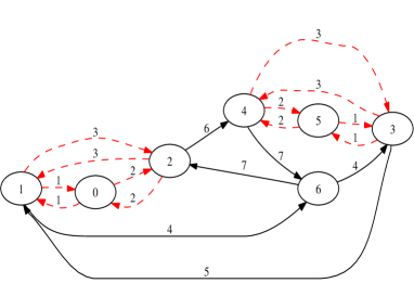
Figure 1: The graph of Example 2.1 (left) and its highway hierarchy for $H=3,L=1$ (right): the dashed lines indicate arcs at level 0, the solid lines indicate arcs at level 1.

2.2 Extension to directed graphs

The original description of the HH algorithm [SS05] applies to undirected graphs only; in this section we provide an extension to the directed case. It should be noted that the HH algorithm was extended to the directed case by the authors (see [SS06]) in a way which is very similar to that described here. However, we believe our slightly different exposition helps to clarify these ideas considerably.

The algorithm for hierarchy construction, as explained in Section 2.1, works with both undirected and directed graphs. However, storing all neighbourhoods $N_{H}^{l}(v)$ for each $v$ and $l$ has prohibitive memory requirements. Thus, the original HH implementation for checking whether a vertex $v$ is in $N_{H}^{l}(u)$ is based on comparing the distance $d(u,v)$ with the “distance-to-border” (also called slack) from $u$ to the border of its neighbourhood $N_{H}^{l}(u)$. The “distance-to-border” $d_{H}^{l}(u)$ is a measure of a neighbourhood’s radius, and is defined as the distance $d(u,v)$ where $v$ is the farthest node in $N_{H}^{l}(u)$, i.e. the cost of the shortest path from $u$ to the $H$-th settled node when applying Dijkstra’s algorithm on node $u$ at level $l$. This is the basis of the slack-based method in [Sch05], p. 19 (from which we draw our notation). In the partial shortest paths tree $B(s_{0})$ computed in Step 2a of the algorithm in Section 2.1, the slack $\Delta(u)$ is recursively computed for all $u\in B(s_{0})$ starting from the leaves $t_{0}$ of $B(s_{0})$, as follows.

1. Initialise a FIFO queue $Q$ to contain all nodes $u$ of $B(s_{0})$, ordering them from the farthest one to the nearest one with respect to $s_{0}$.

2. Set $\Delta(u)=d_{H}^{l}(u)$ for $u$ a leaf of $B(s_{0})$ and $+\infty$ otherwise.

3. If $Q$ is empty, terminate.

4. Remove $u$ from $Q$, and let $p$ be its predecessor in $B(s_{0})$.

5. If $\Delta(p)=+\infty$ and $p\not\in N_{H}^{l}(s_{0})$, $p$ is added to $Q$.

6. Let $\Delta(p)=\min(\Delta(p),\Delta(u)-d(p,u))$.

7. If $\Delta(p)<0$, the edge $(p,u)$ is lifted to the higher hierarchical level.

8. Return to Step 3.

The algorithm works because Thm. 2 in [Sch05] proves that condition $\Delta(p)<0$ is equivalent to the condition of Step 2b of the algorithm in Section 2.1. The cited theorem is based on the following assumption:

$$\forall u\in V\;(u\not\in N_{H}^{l}(t_{0})\rightarrow d_{H}^{l}(t_{0})-d(u,t_{0})<0).$$ (2)

This condition may fail to hold for directed graphs, since $d(u,t_{0})\neq d(t_{0},u)$.

To make Assumption 2 hold, we have to consider a neighbourhood radius computed on the reverse graph, that is the graph $\overline{G}=(V,\overline{A})$ such that $(u,v)\in\overline{A}\Leftrightarrow(v,u)\in A$. Thus, we modified the original implementation to compute, for each node, a reverse neighbourhood $\overline{N}_{H}^{l}(v)$ (see Figure 2), so that we are able to store the corresponding reverse neighbourhood radius $\overline{d}_{H}^{l}(u)\,\forall u\in V$. We replace Step 2 in the algorithm above by:

2a. Set $\Delta(u)=\overline{d}_{H}^{l}(u)$ for $u$ a leaf of $B(s_{0})$ and $+\infty$ otherwise.

We are now going to prove our key lemma.

2.2 Lemma

Let $u,s\in V$ and $t$ a leaf in $B(s)$. If $u\not\in\overline{N}_{H}^{l}(t)$ then $\overline{d}_{H}^{l}(t)-d(u,t)<0$.

Proof.

Suppose $d(u,t)\leq\overline{d}_{H}^{l}(t)$. By definition, this means that there is a shortest path in $\overline{N}_{H}^{l}(t)$ which connects $u$ to $t$. Therefore, $u\in\overline{N}_{H}^{l}(t)$ against the hypothesis. ∎

It is now straightforward to amend Thm. 2 in [Sch05] to hold in the directed case; all other theorems in [Sch05] need similar modifications, replacing $N_{H}^{l}(t)$ with $\overline{N}_{H}^{l}(t)$ and $d_{H}^{l}(t)$ with $\overline{d}_{H}^{l}(t)$ whenever $t$ is target node or is “on the right side” of a path - it will always be clear from the context. The query algorithm must me modified to cope with these differences, using $\overline{d}_{H}^{l}(t)$ instead of $d_{H}^{l}(t)$ whenever we are searching in the backwards direction.

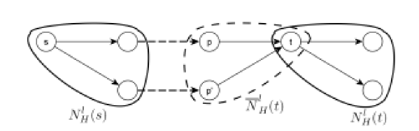
Figure 2: An example which shows neighbourhoods and reverse neighbourhoods with $H=3$; only solid arcs are lifted to a higher level in the hierarchy. Note that arcs $(p,t)$ and $(p^{\prime},t)$ are not lifted even if $p,p^{\prime}\notin N_{H}^{l}(t)$; this is because $p,p^{\prime}\in\overline{N}_{H}^{l}(t)$, and for target node we consider the reverse neighbourhood.

Interestingly, the problem with the slack-based method was first detected when our original implementation of the HH algorithm failed to construct a correct hierarchy for the Paris urban area. This shows that the extension of the algorithm to the directed case actually arises from real needs.

2.3 Heuristic application to dynamic networks

The original Highway Hierarchies algorithm, as described above, finds shortest paths in networks whose arc weights do not change in time. By forsaking the optimality guarantee, we adapt the algorithm to the case of networks whose arc weights are updated in quasi real-time. Whereas the highway hierarchy is constructed using the static arc travelling times from the road network database, each point-to-point path query is deployed on a dynamically evaluated version of the highway hierarchy where the arcs are weighted using the quasi real-time traffic information. In particular, in all tests that involved a comparison with neighbourhood radius we use the static arc travelling times, while for all evaluations of path lengths or of node distances we use the real-time (dynamic) travelling times. This means that the static travelling times are used to determine neighbourhood’s crossings, and thus to determine when to switch to a higher level in the hierarchy, while the key for the priority queue for HH algorithm is computed using only dynamic travelling times.

3 Computational results

In this section we discuss the computational results obtained by our implementation. As there seems to be no other readily available software with equivalent functionality, the computational results are not comparative. However, we establish the quality of the heuristic solutions by comparing them against the fastest paths found by a plain Dijkstra’s algorithm. We mention here two different approaches: dynamic highway-node routing ([SS07]), which uses a selection of nodes operated by the HH algorithm to build an overlay graph (see [HSW06]), and dynamic ALT ([DW07]), which is a dynamic landmark-based implementation of $A^{\ast}$. Both approaches, however, although very performing with respect to query times, require a computationally heavy update phase (which takes time in the order of minutes), and thus are not suitable for our scenario, where, supposedly, each arc can have its cost changed every 2 minutes (roughly).

We performed the tests on the entire road network of France, using a highway hierarchy with $H=65$ and $L=9$. The original network has $7778913$ junctions and $17154042$ road segments; the number of nodes and arcs in each level is as follows.

level	0	1	2	3	4	5	6	7	8	9
nodes	7778913	1517291	433286	182474	91888	53376	34116	23338	16445	11790
arcs	17154042	3461385	1283000	583380	308249	183659	119524	81170	57235	41092

We show the results for queries on the full graph without dynamic travelling times in Table 1; in this case, all paths computed with the HH algorithm are fastest paths. In Table 2, instead, we record our results on a graph with dynamic travelling times; we also report the relative distance of the solution found with our heuristic version of the HH algorithm and the fastest path computed with Dijkstra, and, for comparative reasons, the results of the naive approach which consists in computing the traffic-free optimal solution with the HH algorithm (i.e., on the static graph) and then applying dynamic times on the so-found solution. Dynamic travelling times were taken choosing, for each query, one out of five sets of values recorded in different times of the day for each of the $29384$ arcs with dynamic information.

Although this number is small with respect to the total number of arcs in the graph, it should be noted that most of these arcs correspond to very important road segments (highways and national roads). All arcs $(i,j)$ that did not have a dynamic travelling time were assigned a different weight at each query, chosen at random with a uniform distribution over $[\tau_{ij},15\tau_{ij}]$, where $\tau_{ij}$ is the reference time for arc $(i,j)$. This choice has been made in order to recreate a difficult scenario for the query algorithm: even if the number of arcs with real traffic information is still small, it is going to increase rapidly as the means for obtaining dynamic information increase (e.g. number of road cameras, etc.), and thus, to simulate an instance where most arcs have their travelling time changed several times per hour, we generated each arc’s cost at random. The interval $[\tau_{ij},15\tau_{ij}]$ is simply a rough estimation of a likely cost interval, based on the analysis of historical data. All tables report average values over 5000 queries. All computational results in Table 1 and 2 have been obtained on a multiprocessor Intel Xeon 2.6 GHz with 8GB RAM running Microsoft Windows Server 2003, compiling with Miscrosoft Visual Studio 2005 and optimization level 2.

Computational results show that, although with no guarantee of optimality, our heuristic version of the algorithm works well in practice, with $0.55\%$ average deviation from the optimal solution and a recorded maximum deviation of $17.59\%$; query times do not seem to be influenced by our changes with respect to the original version of the algorithm. The naive approach of computing the shortest path on the static graph, and then applying dynamic times, records an average error of $2\%$, but it has a much higher variance, and a maximum error of $27.95\%$; although the average error is not high, it’s still almost $4$ times the average error of the more sofisticated approach, and the high variance suggests lack of stability in the solution’s quality. The low value recorded for the average error with the naive approach (in absolute terms) can be explained as a consequence of the following two facts: travelling times generated at random on arcs without real-time traffic information cannot simulate real traffic situation, because they lack spatial coherence (i.e. they do not simulate congested nearby zones) and traffic behaviour information (i.e. the fact that during peak hours important road segments are likely to be congested, while less important roads are not), thus making the task of finding a fast path easier; besides, the average query on such a large graph corresponds to a very long path (296 minutes on the traffic-free graph, 2356 minutes on the dynamic graph), and on long paths it is usually necessary to use highways or national roads regardless of their congestion status - which is exactly what the HH algorithm does. This last sentence is supported by the fact that, if we consider only the $500$ shortest queries in terms of path length, the average error of the naive approach increases to $3.60\%$, while the average error of the heuristic version increases to $0.97\%$; this is in accord with the fact that on short paths the influence of traffic is greater, because alternative routes that do not use highways are more appealing, while on long paths using highways is often a necessary step. However, in relative terms, the heuristic version of the HH algorithm performs significantly better than the naive approach proposed for comparison, and we expect the difference to increase (in favour of the heuristic algorithm) if applied to a graph fully covered with real traffic information.

Figure 3 shows how the optimal and the heuristic path may differ; since the hierarchy built on the static graph emphasizes important roads, the heuristic algorithm applied on the dynamically weighted graph still tends to use highways and national roads even when they are congested (up to a certain degree), thus sometimes losing optimality.

	Dijkstra’s algorithm	HH algorithm
# settled nodes	2275563	18966
# explored nodes	2587112	36200
query time [sec]	11.830	0.099

Table 1: Computational results on the static graph: average values

	Dijkstra’s algorithm	HH algorithm	HH algorithm
		naive approach	heuristic version
# settled nodes	2280872	19174	19099
# explored nodes	2594361	36581	36492
query time [sec]	11.917	0.100	0.099
distance from optimum (variance)	0%	2.00% (5.00)	0.55% (0.45)

Table 2: Computational results on the graph with dynamic times: average values

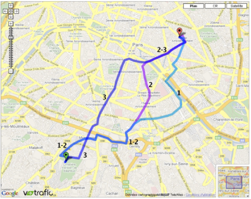
Figure 3: Fast paths calculated with different algorithms; each number identifies a path, paths are partially overlapping. 1: Dijkstra’s algorithm (optimal solution) with real-time arc costs; dynamic travelling time: 24 minutes and 6 seconds. 2: HH algorithm (heuristic solution) with real-time arc costs; dynamic travelling time: 25 minutes and 5 seconds. 3: HH algorithm without real-time arc costs (traffic-free optimal solution); dynamic travelling time: 37 minutes and 5 seconds.

Figure 4: Highway hierarchy near the Champs Elysées, Paris; colour intensity and line width increase with hierarchy level, in that order (a wide line with a lighter colour has a higher hierarchy level than a thin line with dark colour).

4 Conclusion

We present a heuristic algorithm for efficiently finding fast paths in large-scale partially dynamically weighted road networks, and benchmark its application on real-world data. The proposed solution is based on fast multi-level bidirectional Dijkstra queries on a highway hierarchy built on the statically weighted version of the network using the Highway Hierarchies algorithm, and deployed using the dynamic arc weights. Computational results show that, although with no guarantee of optimality, the proposed solution works well in practice, computing near-optimal fast paths quickly enough for our purposes.

References

- [AOPS03] R.K. Ahuja, J.B. Orlin, S. Pallottino, and M.G. Scutellà. Dynamic shortest paths minimizing travel times and costs. Networks, 41(4):197–205, 2003.
- [BRTed] L.S. Buriol, M.G.C. Resende, and M. Thorup. Speeding up dynamic shortest path algorithms. INFORMS Journal on Computing, submitted.
- [CH66] K.L. Cooke and E. Halsey. The shortest route through a network with time-dependent internodal transit times. Journal of Mathematical Analysis and Applications, 14:493–498, 1966.
- [Cha98] I. Chabini. Discrete dynamic shortest path problems in transportation applications: complexity and algorithms with optimal run time. Transportation Research Records, 1645:170–175, 1998.
- [CS02] I. Chabini and L. Shan. Adaptations of the algorithm for the computation of fastest paths in deterministic discrete-time dynamic networks. IEEE Transactions on Intelligent Transportation Systems, 3(1):60–74, 2002.
- [CZ01] E.P.F. Chan and N. Zhang. Finding shortest paths in large network systems. In GIS ’01: Proceedings of the 9th ACM international symposium on Advances in geographic information systems, pages 160–166, New York, NY, USA, 2001. ACM Press.
- [Dea04] B.C. Dean. Shortest paths in fifo time-dependent networks: theory and algorithms. Technical report, MIT, Cambridge MA, 2004.
- [Dij59] E.W. Dijkstra. A note on two problems in connexion with graphs. Numerische Mathematik, 1:269–271, 1959.
- [Dre69] S.E. Dreyfus. An appraisal of some shortest-path algorithms. Operations Research, 17(3):395–412, 1969.
- [DW07] D. Delling and D. Wagner. Landmark-based routing in dynamic graphs. In WEA 2007, volume 4525 of Lecture Notes in Computer Science. Springer, 2007.
- [FHK+05] T. Flatberg, G. Hasle, O. Kloster, E.J. Nilssen, and A. Riise. Dynamic and stochastic aspects in vehicle routing – a literature survey. Technical Report STF90A05413, SINTEF, Oslo, Norway, 2005.
- [GKW05] A.V. Goldberg, H. Kaplan, and R.F. Werneck. Reach for : Efficient point-to-point shortest path algorithms. Technical Report MSR-TR-2005-132, Microsoft Research, 2005.
- [HSW06] M. Holzer, F. Schulz, and D. Wagner. Engineering multi-level overlay graphs for shortest-path queries. In SIAM, volume 129 of Lecture Notes in Computer Science, pages 156–170. Springer, 2006.
- [Ker04] B. S. Kerner. The Physics of Traffic. Springer, Berlin, 2004.
- [NV05] TeleAtlas NV. Tele Atlas Multinet ShapeFile 4.3.1 Format Specifications. TeleAtlas NV, May 2005.
- [Sch05] D. Schultes. Fast and exact shortest path queries using highway hierarchies. Master Thesis, Informatik, Universität des Saarlandes, June 2005.
- [SS05] P. Sanders and D. Schultes. Highway hierarchies hasten exact shortest path queries. In G. Stølting Brodal and S. Leonardi, editors, ESA, volume 3669 of Lecture Notes in Computer Science, pages 568–579. Springer, 2005.
- [SS06] P. Sanders and D. Schultes. Engineering highway hierarchies. In ESA 2006, volume 4168 of Lecture Notes in Computer Science, pages 804–816. Springer, 2006.
- [SS07] P. Sanders and D. Schultes. Dynamic highway-node routing. In WEA 2007, volume 4525 of Lecture Notes in Computer Science, pages 66–79. Springer, 2007.