abstract

M. Khakian Ghomi², M. Bahmanabadi^1,2, F. Sheidaei¹, J. Samimi^1,2, A. Anvari^{1,2 1}Department of physics, Sharif University of Technology,
P.O. box 11365 - 9161, Tehran, Iran.
²ALBORZ Observatory(http://sina.sharif.edu/^∼observatory) sheydaei@sharif.edu

Ultra-High-Energy (UHE) ($E>100~{}$TeV) Extensive Air Showers (EASs) have been monitored for a period of five years ($1997-2003$), using a small array of scintillation detectors in Tehran, Iran. The data have been analyzed to take in to account of the dependence of source counts on zenith angle. Because of varying thickness of the overlaying atmosphere, the shower count rate is extremely dependent on zenith angle. During a calendar year different sources come in the field of view of the array at varying zenith angles and have different effective observation time equivalent to zenith in a day. High energy gamma-ray sources from the EGRET third catalogue where observed and the data were analyzed using an excess method. Upper limits were obtained for 10 EGRET sources [1]. Then we investigated the EAS event rates for these 10 sources and obtained a flux for each of them using parameters of our experiment results and simulations. Finally we investigated the gamma-ray spectrum in the UHE range using these fluxes with reported fluxes of the EGRET sources.
keywords:The EGRET sources, Extensive Air Showers (EASs), Gamma-ray sources, Gamma-ray spectrum

Investigation of Energy Spectrum of EGRET Gamma-ray Sources by an Extensive Air Shower Experiment

M. Khakian Ghomi², M. Bahmanabadi^1,2, F. Sheidaei¹, J. Samimi^1,2, A. Anvari^{1,2 1}Department of physics, Sharif University of Technology,
P.O. box 11365 - 9161, Tehran, Iran.
²ALBORZ Observatory(http://sina.sharif.edu/^∼observatory) sheydaei@sharif.edu

1 Introduction

The EGRET instrument on-board Compton gamma-ray Observatory (CGRO) has detected about 271 high energy ($>100~{}$MeV) gamma-ray sources [2]. Effective sensitivity of EGRET is in the energy range from 100 MeV to 30 GeV.
The EGRET gamma-ray sources in many aspects like characteristics, different energy ranges and etc. have been investigated [3, 4, 5]. Whether the EGRET sources emit gamma-ray at still higher energies or not, is an interesting question. Gamma-rays with energies of about 100 TeV and more, entering the earth atmosphere, produce Extensive Air Shower (EAS) events which could be observed by the detection of the secondary particles of the EAS events on the ground level [6]. This gamma-ray induced EAS events are investigated for diffuse Galactic [7] and extragalactic sources, also Galactic [8], [9] and extragalactic [10] gamma-ray point sources have been investigated too. In this work we have investigated 10 of these point sources.
Our small particle detector array is located at the Sharif University of Technology in Tehran, Iran at about 1200 m above sea level ($\equiv$ 890 g cm^-2). This small array is a prototype for a large EAS array to be built at an altitude of 2600 m ($\equiv$ 756 g cm^-2) at ALBORZ Observatory (AstrophysicaL oBservatory for cOsmic Radiation on alborZ) (http://sina.sharif.edu/ ^∼observatory/) near Tehran. The results of the experiments with this prototype observatory with about $1.7\times 10^{5}$ recorded EAS events was reported earlier [1] and has been shown that some of the EGRET GeV point sources are gamma-ray emitters at energies about 100TeV. Here we report the results of our recent investigation using the data of our earlier experiments to extend the energy spectrum of the observed EGRET sources up to 100TeV and more. In this investigation we present the observational results for 10 EGRET third catalogue sources. Then we investigate the effective area and effective time of observation of each source. Finally we compare the obtained fluxes and spectral indices with the presented fluxes and spectral indices of the EGRET third catalogue sources at the 3rd EGRET catalogue.

2 Experimental arrangement

Our array is constructed of four slab of plastic scintillation detectors ($100\times 100\times 2$ cm³). They are housed in white painted pyramidal boxes [11] which arranged in a square; at 51^∘ 20${}^{{}^{\prime}}$E and 35^∘ 43${}^{{}^{\prime}}$N, elevation 1200 m ($\equiv$ 890 g cm^-2). Two different experimental configurations were used in the experimental set up. The first ($E1$) and the second ($E2$) experimental configurations are identical except the size of the square array. In $E1$ the size is 8.75 m $\times$ 8.75 m and in $E2$ the size is $11.30$ m $\times$ $11.30$ m. More details of the experimental setup is given in the reference [1].

3 Data Analysis

The logged time lags between the scintillation detectors and Greenwich Mean Time (GMT) of each EAS event were recorded as raw data. We synchronized our computer to GMT (http://www.timeanddate.com). Our electronic system has a recording capability of 18.2 times per second. If an EAS event occurs, its three time lags will be recorded and if it does not occur ’zero’ will be recorded. Therefore the starting time of each experiment and the count of records gives us the GMT of each EAS event. We estimated the energy threshold and the mean energy of our experiment and also we calculated the statistical significance of 98 of the 3rd EGRET sources which were in the Field Of View (FOV) of our array.
The complete analysis procedure [1] is itemized as follows:

• The local coordinates: zenith and azimuth angles of each EAS event $(z,\varphi)$ were calculated using a least-square method based on the logged time lags and coordinates of the scintillators. A zenith angle cut off of $60^{\circ}$ is implemented to increase the significance [12].

• The distributions of the local angles of the EAS events were investigated to understand the general behavior of these events. We fitted these distributions with the two functions as follows [13]:

  $$\\ dN=A_{z}\sin z\cos^{n}zdz$$ (1)

  where $A_{z}=95358$ and $n=5.00$, and also

  $$\\ f(\varphi)=A_{\varphi}+B_{\varphi}\cos(\varphi-\varphi_{1})+C_{\varphi}\cos(2\varphi-\varphi_{2})$$ (2)

  where $A_{\varphi}=1,B_{\varphi}=0.081$ , $C_{\varphi}=0.069$, $\varphi_{1}=95^{\circ}$ and $\varphi_{2}=-193^{\circ}$.

• Celestial coordinates (RA,Dec) of each EAS event were calculated using its local coordinates, the GMT of the event and geographical latitude of our array (http://tycho.usno.navy.mil/sidereal.html). Then we calculated galactic coordinates (l,b) of each EAS event from its equatorial coordinates for epoch J2000 [14].

• We estimated the errors in (l,b) of the investigated EGRET sources from the error factors in the array. In this stage we obtained $\bar{r_{e}}=4.35^{\circ}\pm 0.82^{\circ}$ as the mean angular error of our experiment.

• We investigated cosmic-ray initiated EAS events by simulations based on a homogeneous distribution of primary charged particles. These simulations incorporated all known parameters of the experiment. [1]

• We investigated the statistical significance of 98000 random sources and also 98 sources of the 3rd EGRET catalogue, using the method of Li & Ma (Li & Ma 1983) we derived the best-known locations for the EGRET sources in the TeV range [1].

3.1 Shadow of the moon

Observing the shadow of the moon in EAS experiments which usually might have a much larger error circle than the disk of the moon is a very difficult task and requires a careful scrutinization of the data. The difficulty is compounded since a realistic radius for the error circle of the experiment is only obtained by the observation of the shadow which could be indicated as a deficit of shower counts falling in the error circle centered about the moving location of the moon as compared to the average shower counts falling in error circles centered at other positions in sky during the observation time. To carry out the scrutinization of our data, we have proceeded as follows.We have divide our data into sequential time segments and for each time segment we have used the mean values of the local coordinates of moon $(\theta_{m},\varphi_{m})$ moving over our observatory site. These coordinates were obtained using the information provided by the http://aa.usno.navy.mil. Now for an assumed radius of circle of error, angular radius $\rho_{err}$ ranging from $0.5^{\circ}$ to $15^{\circ}$ incremented by $0.5^{\circ}$, we have calculated the number of showers falling in each circle. This has been done by calculating the angular separations $\Theta_{s}$ between the arrival direction of each shower event $(\theta_{s},\varphi_{s})$ and the direction of the moon at the time of recording of that event, using the following equation from spherical geometry:

$$\cos\Theta_{s}=\cos\theta_{m}\cos\theta_{s}+\sin\theta_{m}\sin\theta_{s}\cos(\varphi_{m}-\varphi_{s})$$ (3)

Obviously if $\Theta_{s}<\rho_{err}$ that shower is counted as falling in the moon’s error circle. In order to compare the obtained result with random sampling and scrutinize the difference for each value of $\rho_{err}$ we have chosen 1000 random locations in the sky denoted by local coordinates $(\theta_{r},\varphi_{r})$ and have calculated the number of showers falling in the error circles countered about each of the 1000 random locations. This was similarly done by calculating the angular separation of each shower arrival direction $(\theta_{s},\phi_{s})$ with the direction of the center of the randomly chosen error circle $(\Theta_{r})$ from above equation with $(\theta_{m},\varphi_{m})$ replaced by $(\theta_{r},\varphi_{r})$. If for any shower event $\Theta_{r}<\rho_{err}$ that shower is counted as falling in the error circle of that random position. In these computations (both for the moon as well as for the random locations) a weight factor was used for each of the shower events in order to account for the site-specific effects in our data which depend on the arrival directions of shower events. These effects are :
(1) The different thickness and density of the overlying atmosphere which are effective in shower development and hence its detectability at the height of the observatory.
(2) The geomagnetic effect on the azimuthal arrival direction of the showers. These effects which are specific for each observation site, were separately and independently determined for our site and are reflected in the dependence of the number of shower events on zenithal and azimuthal angles which are given by equations 1 and 2, respectively [13]. To take account of these effects in our observed data, we have assigned a weight factor to each shower arrival direction which is the product of these two independent factors. The weight factor is thus:

$$W(\theta_{s},\varphi_{s})=\cos^{n}\theta_{s}(A_{\varphi}+B_{\varphi}\cos(\varphi-\varphi_{1})+C_{\varphi}\cos(2\varphi-\varphi_{2}))$$ (4)

where the constants n, $A_{\varphi}$,$B_{\varphi}$ and $C_{\varphi}$ are given below Eqs.1 and 2.
It should be remembered that in our earlier work, [1] reporting the observation of EGRET gamma-ray point sources in TeV data by excess method, both of these effects were carefully taken into account by determining the exposure map of our observations by simulations incorporating these effects along with other particularities of our observations and by correcting of our observed data by dividing it by the exposure map in galactic coordinates.

3.2 Distributions of number of EAS events in error circles

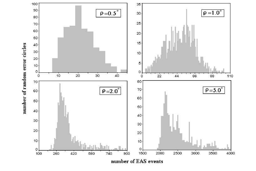
Figure 2: Histograms show the frequency of circles of error with radius $\rho$ and random chosen centers in the sky vs. the number of EAS events falling in each error circle.

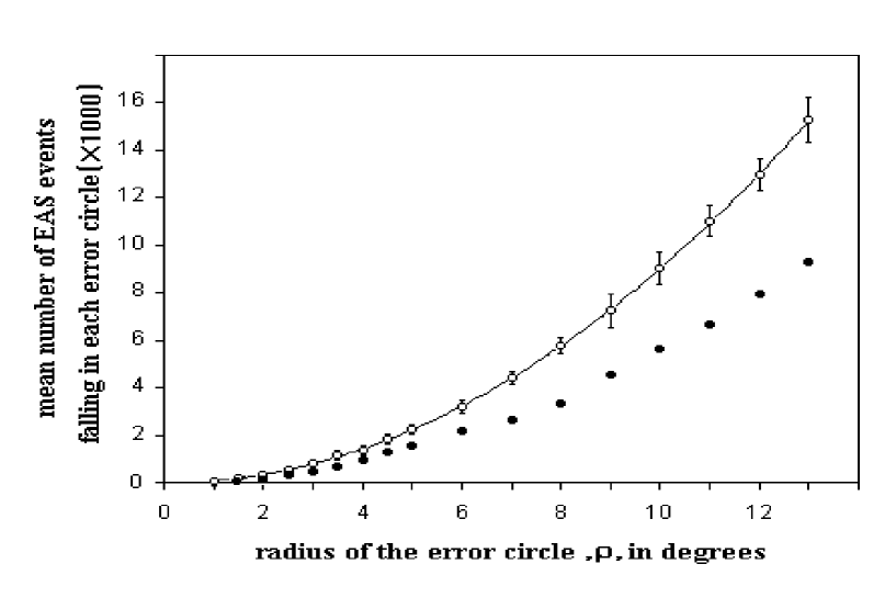
Figure 3: Dependence of the mean number of EAS events falling in the random error circles as a function of the radius of the error circle, $\rho$. Smooth curve shows a $\rho^{2}$ dependence. Error bars are the standard deviation of the distribution shown in Fig.2, and statistical errors for the moon. Open circles $(\circ)$ are random error circles. Filled circles$(\bullet)$ are error circles centered about the location of the moving moon.

Here we discuss the distribution of number of EAS events falling in the error circles of different radii as determined according to the aforementioned procedure. We first present the results for each of the sets of 1000 randomly chosen error circles. Fig.2 shows the histogram of frequency of occurrence of number of circles with respect to the number of EAS falling in the error circle. The histograms distributions corresponding to different radii of error circles are shown here as illustration. These for other radii show similar distributions and all these distributions nearly fit gaussian distributions with a mean and a variance which increase with increasing radius. This result is very assuring and shows the correctness of our sophisticated numerical procedure and the validity of using the mean number of events, in these randomly chosen locations of error circles in the sky to compare with the number of events falling in the error circle countered about the moving moon. Fig.3 shows the variation of the mean number of events of these distribution as a function of the chosen radius of the error circles. It is seen that these calculated means show a nearly exact dependence on the square of the radius. This result is not surprising and is exactly what one would expect to get from a correct random sampling of statistical data. However, in view of the complexity and sophistication involved in our entire procedure (with inclusion of the weight factors), this result is again very assuring and shows that we can use these mean number of events to compare with that falling in the error circles centered about the moving moon and rule out the possibility of the deficit in the number of events falling in the moon centered circle as due to statistical fluctuation. In Fig.3 we have also shown the number of events falling in the moon-countered circles for comparison with the means of the random samplings. It is seen that in every case( for every chosen error circle radius) the deficit of number of EAS from the direction of the moving moon is quite significant as compared to the error bars of the mean of random sampling( Fig.3) which is taken as the variance of nearly gaussian distributions of Fig.2. As seen here the deficit which is from 1.6 to about 7.1 times the standard deviation of the mean of random distributions is quite significant and since it is definitely associated with the moving moon it must be associated with some moon- related phenomenon. We will not discuss this phenomenon here and rather simply call it the shadow of the moon in our EAS observed data.

3.3 Estimation of energy thresholds

Our detected EAS events are a mixture of cosmic-ray and gamma-ray events. In $E1$ the total number of EAS events was 53,907 and the duration of the experiment was 501,460 seconds. So the mean event rate of the first experiment was 0.1075 events per second. The distribution of the time between successive events was investigated and found to be in good agreement with an exponential function, indicating that our event sampling is completely random [16]. In $E2$ the total number of events was 173,765 and the duration of the second experiment was 2,902,857 seconds, so its mean event rate was 0.05986 events per second.
We refined the data to separate out the acceptable events. Events are acceptable if there is a good coincidence between the four scintillator pulses, also we omitted the events with zenith angles more than 60^∘ because of their less accuracy. Therefore after these separations we obtained smaller data sets of 46,334 and 120,331 events for $E1$ and $E2$ respectively. Since we cannot determine the energy of the showers on an event by event basis, we estimate our lower energy threshold by comparing our event rate to the following cosmic-ray integral spectrum [17],

$$J(E)=2.78\times 10^{-5}E^{-2.22}+9.66\times 10^{-6}E^{-1.62}$$

$$\hskip 28.45274pt-1.94\times 10^{-12}\hskip 8.53581pt40\leq E\leq 5000\hskip 2.84526pt{\rm TeV}$$ (5)

The obtained lower energy limits are 39 TeV in $E1$ and 54 TeV in $E2$. The calculated mean energies with above energy spectrum are 94 and 132 TeV in $E1$ and $E2$, respectively. Since the distribution of cosmic-ray events within the array around these energy ranges is homogeneous and isotropic, we used an excess method [18] to find signatures of the EGRET 3rd catalogue gamma-ray sources. This method was used for both $E1$ and $E2$.

4 Calculation of effective area and time

Number of secondary particles in the growth profile of EAS events increases in atmosphere until the shower maximum and then decreases after it. In energy of about 100 TeV the shower maximum height is at about 500g cm^-2 and a fraction of these secondary particles arrive to the ground level particle detectors of our array at Tehran level (1200 m$\equiv$ 890 g cm^-2).
For calculating the effective surface of each experiment ($E1$ and $E2$) we used Greisen lateral distribution of electrons which is known the NKG formula [19] and CORSIKA simulation code [20] for the simulation of the two sets of proton showers with energy thresholds of 39 TeV and 54 TeV respectively for $E1$ and $E2$ at our array level. From our logged EAS events we obtained a zenith distribution function for $E1$ and $E2$, which the mean zenith angles are $26^{\circ}$ for both of them. Also we calculated the $\bar{z}$ which was obtained from the weight curve of the zenith distribution $dN/dz\propto\cos^{n}z\sin{z}$ and we obtained the $26^{\circ}$ too. This weight curve was obtained by fitting the function $dN/dz$ to our data in the $E1$ and $E2$ with $n=5.00$. So in the first approximation we used the effective thickness of the passed atmosphere as $890{\rm g~{}cm}^{-2}/\cos(26^{\circ})=980{\rm g~{}cm}^{-2}$. In the thickness, the average number of the secondary particles for the two experiments are $N_{E1}=5265$ and $N_{E2}=8571$, these two numbers obtained from 1000 simulated proton showers for each energy threshold. So based on the NKG formula the mean effective surfaces of EAS events at Tehran level are $965~{}{\rm m}^{2}$ and $2173~{}{\rm m}^{2}$ for $E1$ and $E2$ respectively. With these results we could obtain the mean effective surface of our array in the upper level of the atmosphere (The surface that if a primary particle passes through it, the array could detect its EAS events) $718{\rm m}^{2}$ and $1751{\rm m}^{2}$ for $E1$ and $E2$ respectively.
For calculation of the effective time of observation of each source in every 24 hours, we used the spherical geometry and the track of each source in the local coordinates. Each source with its celestial coordinates right Ascention, Declination (RA,Dec) is introduced in the 3rd EGRET catalogue. Time duration of each source is calculated by reaching the source to the zenith angle of $60^{\circ}$ from the direction of east to the same zenith angle from the west, and the distribution function $dN/dz=\propto\cos^{n}z\sin{z}$ which is related to the zenith distribution effect [1]. Finally we obtained the mean effective time of observation of our array for all 10 sources equivalent to 4h,28${}^{{}^{\prime}}$ (equivalent to existence of 4$h$,28${}^{{}^{\prime}}$ the source at zenith) for every 24 hours. The FOV of our array with the $60^{\circ}$ zenith angle cutoff is $\pi$ steradian. With these calculated factors we obtained fluxes(events cm^-2s^-1sr^-1) for each of the 10 sources in $E1$ and $E2$ which are shown in Table 1.

5 Results

Our results have been compared with the EGRET results. For each source we have fluxes and energies from EGRET, $E1$ and $E2$, so we extracted a spectral index for each source and compared it with the reported spectral index of EGRET. Some information about the 10 EGRET sources like Name, RA, Dec, and spectral index and its error, $(\gamma\pm\Delta\gamma)_{EGT}$, are from the 3rd EGRET catalogue [2]. Other information like mean energy for $E1$ and $E2$ which are 94TeV and 132TeV respectively (are not shown in the table), fluxes of the two experiments and spectral indexes and their errors, $(\gamma\pm\Delta\gamma)_{OUR}$, have been calculated in this analysis. The last column shows the agreement of our spectral indices to its in the 3rd EGRET catalogue.

5.1 Result of Energy Analysis with Simulated Showers

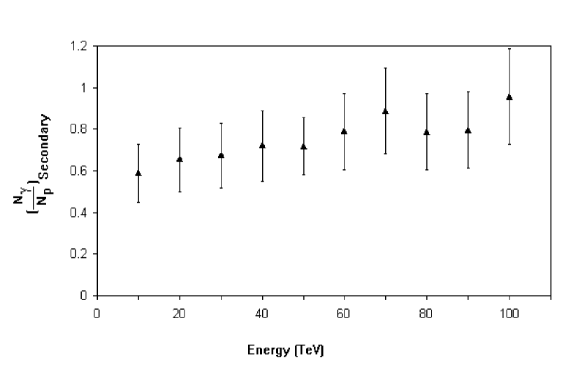
Figure 4: The ratio of the mean number of secondary charged particles at the location of our site produced in gamma-ray generated simulated Extensive Air Shower to that produced by proton generated showers as a function of the energy of the primary radiation( Gamma-ray and proton) entering the top of the atmosphere.

For further energy analysis of our measured data of EAS events observed at our site we have used the CORSIKA code[20] to simulate showers with the inclusion of geomagnetic field pertinent to the location of our site from data provided by http://www.ngdc.noaa.gov. We have simulated a total of 7350 showers entering the top of atmosphere at various zenith angles $(0^{\circ},15^{\circ},30^{\circ},45^{\circ},60^{\circ})$ and for each zenith angle at 12 various azimuth angles ranging from $0^{\circ}$ to $360^{\circ}$ every $30^{\circ}$. For each angle the simulations were repeated 10 times for energies less than 50 TeV and 5 times for energies greater than 50 TeV with separately 10 TeV intervals from 10 TeV to 100 TeV. These simulations were carried out similarly for entering protons as well as gamma-rays. For each simulation the number of secondary charged particles of the simulated shower at the height of observation of our site was determined from CORSIKA code. In order to make an energy analysis comparing gamma-ray initiated showers with those initiated by protons in our observations we have calculated a mean number of secondary shower particles for each energy by averaging over all the angles using the site-specific weight factor discussed in sec 3.1(Eq. 4). The ratio of angle-averaged mean of number of secondary charged particles in gamma-ray initiated showers to that of the mean for proton-initiated showers is shown in Fig.4 as a function of energy in the energy range of our simulations. The ratio shown here incorporates almost all of related particularities of our experiments. Since in our observations we have used exactly identical experimental procedure, equipment, thresholds and set-ups for all of the recorded showers irrespective of the nature of the radiation which initiates the shower the relative detection efficiency of our array and observations could only depend on the ratio of these means depicted in Fig.4. Now we use the relative detection efficiency calculated from simulated data and shown in Fig.4 to estimate the relative number of gamma-ray initiated showers to that initiated by protons, using the known energy spectrum of proton showers of the form

$$\frac{dN_{p}}{dE}=N_{p10}(\frac{E}{10TeV})^{-\Gamma_{p}}.$$ (6)

Where $dN_{p}$ is the number of proton showers in the energy interval $E$ to $E+dE$, $N_{p10}$ is a constant and $\Gamma_{p}$ is the spectral index of EAS producing protons. Now denoting our array’s relative detection efficiency by $\eta(E)$, we can write for the expected differential number of gamma-ray initiated showers:

$$\frac{dN_{\gamma}}{dE}=\eta(E)N_{p10}(\frac{E}{10TeV})^{-\Gamma\gamma}$$ (7)

where $\Gamma_{\gamma}$ is the spectral index of EAS producing gamma- rays. Dividing Eq.7 by Eq.6 and upon integration from a threshold energy to infinity, the ratio of observed gamma-ray EAS events to that initiated by protons is obtained. Thus we write:

$$\frac{N_{\gamma EAS}}{N_{pEAS}}=\frac{\int^{\infty}_{E_{t}}\eta(E)E^{-\Gamma_{\gamma}}\,dE}{\int^{\infty}_{E_{t}}E^{-\Gamma_{p}}\,dE}$$ (8)

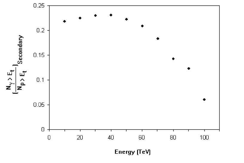
Figure 5: The ratio of the mean number of gamma-ray generated showers to that of proton generated showers expected to be observed at our site as a function of the threshold energy of our experiments.

where $E_{t}$ is assumed threshold energy. For the energy range covered in this analysis, we use $\Gamma_{p}=2.7$ and for gamma-ray spectral index we use the mean value of the spectral indices that we have estimated above (Table.1) for the sources with the highest statistical significance (those observed at a statistical significance level of higher than $1.5\sigma$). Thus using our estimations of table 1 we have $\Gamma_{\gamma}=2.3$. In order to carry out the integrations in Eq.8 we are forced to impose a truncation since with our rather limited computer shower simulations we only have $\eta(E)$ for $10TeV<E<100TeV$. For the sake of numerical consistency, we have imposed this truncation to E=100 TeV in the denominator of Eq.8 as well as its numerator. The result of these calculations obviously depend on the value of an assumed threshold energy, $E_{t}$, therefore the numerical calculations were repeated for values of $E_{t}$ from 10 TeV to 100 TeV with 10 TeV intervals. The result of these calculations, that is, the ratio of the number of gamma-ray EAS events to that of proton EAS events expected to be detected in our experiments at our site is shown as a function of the threshold energy in Fig.5. Here we see that this ratio shows a maximum at a value of $E_{t}=40\,TeV$ which very nearly corresponds to the lower value of the two threshold energies of our two experiments.

Name($3EG\hskip 2.84526ptJ$)	RA,Dec	$ID$	$(\gamma\pm\Delta\gamma)_{EGT}$	$\log{F_{E1}}$	$\log{F_{E2}}$	$(\gamma\pm\Delta\gamma)_{OUR}$	$|\gamma_{OUR}-\gamma_{EGT}|$
0237+1635	39.3,16.5	A	1.85$\pm$0.12	-11.25	-11.53	1.90$\pm$0.27	0.05
0407+1710	61.8,17.1		2.93$\pm$0.37	-10.77	-11.45	4.20$\pm$0.40	1.27
0426+1333	66.6,13.5		2.17$\pm$0.25	-11.11	-11.28	1.15$\pm$0.48	1.02
0808+5114	122.1,51.2	a	2.76$\pm$0.34	-11.01	-11.58	3.87$\pm$0.42	1.11
1104+3809	126.1,38.1	A	1.57$\pm$0.15	-11.10	-11.72	4.21$\pm$0.50	2.64
1308+8744	197.0,87.7		2.17$\pm$0.66	-10.96	-11.53	3.87$\pm$0.45	1.70
1608+1055	242.1,10.9	A	2.63$\pm$0.24	-10.92	-11.72	4.34$\pm$0.50	1.71
1824+3441	276.2,34.6		2.03$\pm$0.50	-10.65	-11.25	4.07$\pm$0.35	2.04
2036+1132	309.1,11.5	A	2.83$\pm$0.26	-11.08	-11.73	4.41$\pm$0.53	1.58
2209+2401	332.4,24.0	A	2.48$\pm$0.50	-10.91	-11.31	2.71$\pm$0.42	0.23

Table 1: Comparison of our spectral indices of the 10 sources with the spectral indices of them which is introduced by the 3rd EGRET catalogue. The last column shows agreement of our spectral indices to EGRET spectral indices.

6 Concluding remarks

We believe the main reasons for success in these observations and investigations on EGRET gamma-ray point sources despite the low statistics of $\sim 3\times 10^{5}$ EAS events from our small array of ALBORZ prototype observatory, relies on the following two favorite points of strength:
(1) we have intensively studied the location- dependent factors which influence shower development and shower count from various angular bins in the sky. These factors are the mass of the overlying atmosphere and anisotropy in azimuth angles which it is attributed to the effect of the geomagnetic field [21], [13], [22]. For our particular site we investigated these effects which are in form of Eqs. 1 and 2. We carefully refined our data from these effects finally the investigation of the EGRET gamma-ray point sources are based on the corrected data.
(2) Our site and the duration of our observations in the data set have been such that 10 of the EGRET gamma-ray point sources have crossed our site at small enough zenith angles to make their observation possible at least with a statistical significance of $1.5\sigma$ with Li and Ma criterion in the excess method which we have used[1]. In order to investigate this rather fortunate point for our site and the time of these observations, we have calculated the average zenith all angle of passage of each of 271 EGRET gamma-ray point sources during our entire observation period, for each of these sources. We have also calculated the statistical significance(number of sigma) for excess counts from these sources. The result is shown here in Fig.1 and it convincingly shows an inverse correlation between the statistical significance of excess shower counts from the EGRET point source location and the average zenith angle of the transit of the source over our site. The computed coefficient of this correlation(correlation between inverse statistical significance and $\overline{z}$) is 0.77.
Obviously the EGRET sources investigated here are those with highest statistical significance corresponding to the lowest zenith angles of the passage of the source over our site.
Our results shows that our spectral indices within error limits are in agreement with EGRET spectral indices for most of the considered here.
For the calculation of the effective area of the EAS events at first , we calculated the primary particle energy, then we extracted the number of the secondary particles from a set of CORSIKA simulations, and finally we used the Greizen lateral distribution for these particles. In the near future with a larger array and larger set of logged EAS events at ALBORZ observatory we hope to calculate these results more accurately.
It is worth remarking that due to increased probability of pair- production interaction of VHE and UHE gamma-rays with various low energy universal photons, the absorption of these gamma-rays becomes significant for sources located at cosmological distances. This absorption has been studied extensively [23, 24, 25]. The lack of observation of VHE and UHE gamma-rays from extragalactic EGRET gamma-ray sources has been generally attributed to the absorption of the gamma-rays from these sources which are located at cosmological distances.
Stecker and De Jager (1997) gave a parametric relation for optical depth $(\tau_{j})$ as a function of the source gamma energy $(E_{TeV})$ and red shift (z) for the two models (j=1,2) they have studied. For the 39TeV energy threshold of our experiments, we use their parametric relation with an optical depth of unity to calculate the red shift of the sources we have observed in our EAS experiments and have investigated here(Table 1). The result is z=0.0032 for their model 1 and z=0.0024 for their model 2. Ong,[26] have listed the red shifts of two classes of EGRET extragalactic sources and the calculated red shifts for the sources investigated here is smaller than red shifts listed for these classes of objects. However, we should remark that the recent discovery of the unexpected by hard spectra of the Blazar sources observed in HESS data [27] bear as the possibility of observation of EGRET gamma-ray point sources at higher energies. It would be open for future ground-base observations.
The energy analysis carried out here using simulated shows with CORSIKA has shown that the ratio of number of gamma-ray generated EAS events expected to be detected at our site relative to the number of proton- generated EAS events show a maximum at a value of 40 TeV for the threshold energy of observation of EAS events at our site. The fortunate fact that this value corresponds to the lower value of the threshold energies of our two experiments, provides further support for the fact that the data collected in our experiments at our site has had this extra advantageous attribute for the observation of gamma-ray initiated EAS events in the 10 TeV to 100 TeV energy range and thus the extra advantage for observing gamma-ray point sources in this range.

7 acknowledgements

This research was supported by a grant from the national research council of Iran for basic sciences. The many useful and conductive comments by anonymous referee is very much appreciated. Also many thank from Prof. James Matthews for his comments and attentions to our works at ICRC 2005, Pune, India.

References

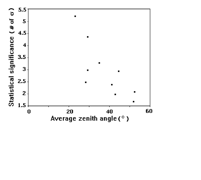
Figure 1: Distribution of statistical significance versus average zenith angle of transit of calculated for 271 EGRET gamma-ray sources over our site(only sources with significance $>1.5\sigma$ are shown.).

References

- [1] Khakian Ghomi, M., Samimi, J., Bahmanabadi, M., 2005, A&A, 434, 459
- [2] Hartman, R.C., et al., 1999, ApJ, 123, 79
- [3] Bhattacharia, D., Akyuse A., Miyagi T., Samimi J., 2003, A&A, 404, 163
- [4] Cillis, A.N., Hartman R.C., 2005 ApJ, 621, 291C
- [5] Zhang, S., Collmar, W. , Hermsen, W., Schonfelder, V., 2004, A&A, 421, 983Z
- [6] Gaisser, T.K., , Cambridge Univ Press, New York, (1990)
- [7] Brezinskii, V.S., Kudriavtsev, V.A., 1990, ApJ 349, 620B
- [8] Atkins, R., Benbow, W., Berlay, D. et al., 2005, PhRvL 95y, 1103A
- [9] McKay, T.A., Borione, A., Catanese, M. et al., 1993, ApJ 417, 742
- [10] Fidelis, V.V., Neshpor, Yu.I., Eliseev, V.S. et al., 2005, A&A 24, 53F
- [11] Bahmanabadi, M., et al. 1998, Experimental Astronomy, 8, 211
- [12] Mitsui, K., et al., 1990, Nucl. Inst. Meth., A290, 565
- [13] Bahmanabadi, M., et al. 2002, Experimental Astronomy, 13, 39
- [14] Roy, A.E., Clarke, D., , (Adant Hilger, Glasgow, 1991)
- [15] Li, T., Ma, Y., 1983, ApJ, 272, 317
- [16] Bahmanabadi, M., et al. 2003, Experimental Astronomy, 15, 13
- [17] Borione, A., et al. 1997, ApJ, 481,313
- [18] Amenomori, M., et al., 2002, ApJ, 580, 887
- [19] Kamata, K., Nishimura, J. (1958) Prog. Theor. Phys.(kyoto) suppl. 6, 93
- [20] Heck, D., et al., Report FZKA 6019(1998), Forschungszentrum Karlsruhe http://www-ik.fzk.de/corsika/physics-description/corsika-phys.html
- [21] Ivanov, A.A. et al., 1999, JETP Let. 69, 288-293
- [22] He, H.H., Sun, B.G., Zhou, Y., 2005, ICRC, India, 6, 5-8
- [23] Stecker, F.W, Cosmic Gamma ray, Moro Book Corp., Baltimore (1971)
- [24] Fazio, G.G., Stecker, F.W., 1970, Nature, 226, 135
- [25] Stecker, F.W., De Jager, O.C, 1997, ApJ, 476, 716
- [26] Ong, R.A., et al., 2001, ICRC, Germany, 2593.
- [27] Aharonian , F., et al., Nature 440(2006) 1018-1021