SW Sextantis stars: the dominant population of CVs with orbital periods between 3–4 hours

Abstract

We present time-series optical photometry of five new CVs identified by the Hamburg Quasar Survey. The deep eclipses observed in HS 0129+2933 (= TT Tri), HS 0220+0603, and HS 0455+8315 provided very accurate orbital periods of 3.35129827(65), 3.58098501(34), and 3.56937674(26) h, respectively. HS 0805+3822 shows grazing eclipses and has a likely orbital period of 3.2169(2) h. Time-resolved optical spectroscopy of the new CVs (with the exception of HS 0805+3822) is also presented. Radial velocity studies of the Balmer emission lines provided an orbital period of 3.55 h for HS 1813+6122, which allowed us to identify the observed photometric signal at 3.39 h as a negative superhump wave. The spectroscopic behaviour exhibited by all the systems clearly identifies them as new SW Sextantis stars. HS 0220+0603 shows unusual N ii and Si ii emission lines suggesting that the donor star may have experienced nuclear evolution via the CNO cycle.

These five new additions to the class increase the number of known SW Sex stars to 35. Almost 40 per cent of the total SW Sex population do not show eclipses, invalidating the requirement of eclipses as a defining characteristic of the class and the models based on a high orbital inclination geometry alone. On the other hand, as more SW Sex stars are identified, the predominance of orbital periods in the narrow 3–4.5 h range is becoming more pronounced. In fact, almost half the CVs which populate the 3–4.5 h period interval are definite members of the class. The dominance of SW Sex stars is even stronger in the 2–3 h period gap, where they make up 55 per cent of all known gap CVs. These statistics are confirmed by our results from the Hamburg Quasar Survey CVs. Remarkably, 54 per cent of the Hamburg nova-like variables have been identified as SW Sex stars with orbital periods in the 3–4.5 h range. The observation of this pile-up of systems close to the upper boundary of the period gap is difficult to reconcile with the standard theory of CV evolution, as the SW Sex stars are believed to have the highest mass transfer rates among CVs.

Finally, we review the full range of common properties that the SW Sex stars exhibit. Only a comprehensive study of this rich phenomenology will prompt to a full understanding of the phenomenon and its impact on the evolution of CVs and the accretion processes in compact binaries in general.

1 Introduction

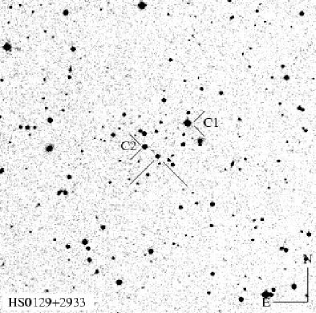
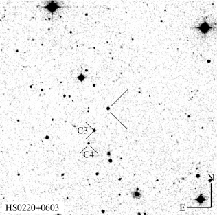
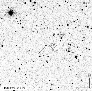
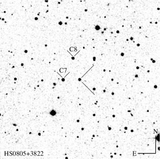
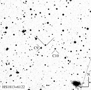
Figure 1: $10\arcmin\times 10\arcmin$ finding charts for HS 0129+2933, HS 0220+0603, HS 0455+8315, HS 0805+3822, and HS 1813+6122 obtained from the Digitized Sky Survey. See Table 2 for details on the comparison stars C1–C10.

The Palomar-Green (PG) survey (Green, Schmidt & Liebert 1986) led to the identification of several relatively bright ($V\sim 15$), deeply eclipsing cataclysmic variables (CVs) with orbital periods in the range $3-4$ h, namely SW Sex (Penning et al., 1984), DW UMa (Shafter, Hessman & Zhang 1988), BH Lyn (Thorstensen et al., 1991; Dhillon et al., 1992), and PX And (Thorstensen et al., 1991). Szkody & Piché (1990) and Thorstensen et al. (1991) established a number of common traits among these systems, including unusually “V”-shaped eclipse profiles, the presence of He II $\lambda$4686 emission, a substantial orbital phase lag ($\sim 0.2$ cycle) of the radial velocities of the Balmer lines with respect to the motion of the white dwarf, and single-peaked emission lines that display central absorption dips around orbital phases $\simeq 0.4-0.7$. The “SW Sex phenomenon” was later extended to lower orbital inclinations after the identification of several grazingly eclipsing and non-eclipsing CVs which exhibit the spectroscopic properties characteristic of the SW Sex class (WX Ari: Beuermann et al. 1992; Rodríguez-Gil et al. 2000; V795 Her: Casares et al. 1996; LS Peg: Martínez-Pais, Rodríguez-Gil & Casares 1999; Taylor, Thorstensen & Patterson 1999; V442 Oph: Hoard, Thorstensen & Szkody 2000).

The observational characteristics of the SW Sex stars are not easily reconciled with the properties of a simple, steady-state hot optically thick accretion disc which is expected to be found in intrinsically bright, weakly-magnetic CVs above the period gap. Nevertheless, a variety of mechanisms have been invoked to explain the behaviour of the SW Sex stars, such as stream overflow (Hellier & Robinson, 1994; Hellier, 1996), magnetic white dwarfs (Williams, 1989; Casares et al., 1996; Rodríguez-Gil et al., 2001; Hameury & Lasota, 2002), magnetic propellers in the inner disc (Horne, 1999), and self-obscuration of the inner disc (Knigge et al., 2000). While no unambiguous model for their accretion geometry has been found so far, it is becoming increasingly clear that the SW Sex stars are not rare and unusual systems, but represent an important, if not dominant fraction of all CVs in the orbital period range $3-4$ h (Rodríguez-Gil, 2005; Aungwerojwit et al., 2005). Hence, a thorough investigation of this class of systems is important in the context of understanding CV evolution as a whole.

In this paper, we present five new CVs identified in the Hamburg Quasar Survey (HQS; Hagen et al. 1995) which are classified as new SW Sex stars on the basis of our follow-up photometry and spectroscopy. The new discoveries bring the total number of confirmed SW Sex stars to 35, and we discuss the global properties of these objects as a class.

Figure 2: Flux-calibrated optical spectra of the five new CVs.

Table 1: Properties of the five new SW Sex stars. The coordinates and the $B$ and $R$ magnitudes were taken from the USNO-B catalog (Monet et al., 2003). The $J$, $H$, and $K_{\mathrm{s}}$ magnitudes were taken from the 2MASS catalogue. The emission line parameters are measured from the public SDSS spectrum.

	HS 0129+2933	HS 0220+0603	HS 0455+8315	HS 0805+3822	HS 1813+6122
Right ascension (J2000)	$01^{\mathrm{h}}31^{\mathrm{m}}59.86^{\mathrm{s}}$	$02^{\mathrm{h}}23^{\mathrm{m}}01.65^{\mathrm{s}}$	$05^{\mathrm{h}}06^{\mathrm{m}}48.27^{\mathrm{s}}$	$08^{\mathrm{h}}09^{\mathrm{m}}08.40^{\mathrm{s}}$	$18^{\mathrm{h}}14^{\mathrm{m}}29.83^{\mathrm{s}}$
Declination (J2000)	$+29\degr 49\arcmin 22.3\arcsec$	$+06\degr 16\arcmin 50.0\arcsec$	$+83\degr 19\arcmin 23.3\arcsec$	$+38\degr 14\arcmin 06.5\arcsec$	$+61\degr 23\arcmin 34.5\arcsec$
Orbital period (h)	3.35129827(65)	3.58098501(34)	3.56937674(26)	$\simeq 3.22$	$\simeq 3.38$
$B/R$ magnitudes	15.3 / 14.7	16.5 / 16.2	15.2 / 14.6	14.7 / 14.6	15.1 / 14.5
$J/H/K_{\mathrm{s}}$ magnitudes	14.6 / 14.4 / 14.3	15.4 / 15.1 / 14.8	14.4 / 14.3 / 14.1	15.3 / 15.2 / 14.9	14.8 / 14.7 / 14.6
${\mathrm{H}\alpha}$ EW [Å] / FHWM [$\mathrm{km\,s^{-1}}$]	61 / 1160	73 / 1390	50 / 1180	25 / 1040	22 / 1050
${\mathrm{H}\beta}$ EW [Å] / FHWM [$\mathrm{km\,s^{-1}}$]	25 / 1265	43 / 1560	29 / 1250	11 / 970	6 / 1020
${\mathrm{H}\gamma}$ EW [Å] / FHWM [$\mathrm{km\,s^{-1}}$]	16 / 1350	25 / 1545	31 / 1540	10 / 1010	5 / 930
He I $\lambda$5876 EW [Å] / FHWM [$\mathrm{km\,s^{-1}}$]	8 / 1120	15 / 1270	– / –	2 / 720	1 / 720
He I $\lambda$6678 EW [Å] / FHWM [$\mathrm{km\,s^{-1}}$]	5 / 1090	9 / 1240	10 / 1240	4 / 830	– / –
He II $\lambda$4686 EW [Å] / FHWM [$\mathrm{km\,s^{-1}}$]	– / –	6 / 2190	17 / 1900	4 / 700	– / –

2 Observations and data reduction

2.1 Identification

The five new CVs (Fig. 1) were selected for follow-up observations upon the detection of emission lines in their HQS spectra. Identification spectra of HS 0220+0603, HS 0805+3822, and HS 1813+6122 were respectively obtained in October 1990 with the Calar Alto 3.5-m telescope, in December 1996 with the 1.5-m Tillinghast telescope at Fred Lawrence Whipple Observatory, and in June 1991 with the Calar Alto 2.2-m telescope as part of QSO and galaxy searches. HS 0129+2933 and HS 0455+8315 were both identified as CVs in September 2000 using the Calar Alto 2.2-m telescope as part of a dedicated search for CVs in the HQS (Gänsicke et al., 2002).

HS 0129+2933 (= TT Tri) was already identified as an eclipsing star by Romano (1978). At the time of writing this paper we were aware of a multicolour photometric study by Warren, Shafter & Reed (2006), in which an eclipse ephemeris is derived for the first time.

HS 0805+3822 was independently found as a CV in the Sloan Digital Sky Survey (SDSS J080908.39+381406.2, Szkody et al. 2003) and was identified as a SW Sex star.

Flux-calibrated, low resolution identification spectra of the five new CVs are shown in Fig. 2. The spectra are dominated by strong, single-peaked Balmer and He i emission lines on top of blue continua. The high excitation emission lines of He ii $\lambda$4686 and the C iii/N iii Bowen blend near 4640 Å are also observed, and are especially intense in HS 0455+8315. Table 1 summarises some properties of the new CVs.

Table 2: Comparison stars used for the differential CCD photometry (see Fig. 1).

ID	USNO-A2.0	$R$	$B$
C01	1125-00509642	13.3	14.0
C02	1125-00510117	14.8	15.2
C03	0900-00553937	15.8	17.7
C04	0900-00554015	16.4	18.9
C05	1725-00217755	13.8	15.1
C06	1725-00218117	15.4	15.9
C07	1275-07186372	15.0	15.0
C08	1275-07186091	15.7	17.2
C09	1500-06459684	14.6	15.1
C10	1500-06458763	15.8	16.5

2.2 Optical photometry

We obtained differential CCD photometry of the five new CVs at seven different telescopes: the 2.2-m telescope at Calar Alto Observatory, the 1.2-m telescope at Kryoneri Observatory, the 0.82-m IAC80 and the 1-m Optical Ground Station at Observatorio del Teide, the 0.7-m telescope of the Astrophysikalisches Institut Potsdam, the 1.2-m telescope at Fred Lawrence Whipple Observatory, and the 0.7-m Schmidt-Väisälä telescope at Tuorla Observatory, and the 0.35-m telescope at West Challow Observatory. Details on the instrumentation are given in the notes to Table 3, which also contains the log of the photometric observations. The data obtained at Calar Alto, Kryoneri, and Tuorla were reduced with the pipeline described by Gänsicke et al. (2004), which applies bias and flat-field corrections in MIDAS and then uses Sextractor (Bertin & Arnouts, 1996) to extract aperture photometry for all objects in the field of view. The reduction of the AIP data was carried out completely using MIDAS. IRAF was used to correct the OGS, IAC80, and FLWO data for the bias level and flat-field variations, and to compute Point Spread Function (PSF) magnitudes of the target and comparison stars. Fig. 1 shows finding charts for the five new CVs and indicates the comparison stars used for differential photometry. The USNO $R$ and $B$ magnitudes of the comparison stars are given in Table 2. Sample light curves are shown in Fig. 4. HS 0129+2933, HS 0220+0603, and HS 0455+8315 are deeply eclipsing, HS 0805+3822 displays evidence for grazing eclipses (similar to WX Ari, Rodríguez-Gil et al. 2000), and all five systems show substantial short time-scale variability. From the scatter in the comparison star light curves we estimate that the differential photometry is accurate to 1 per cent.

2.3 Optical spectroscopy

The spectroscopic data were obtained with five different telescopes: the 2.5-m Isaac Newton Telescope (INT) and the 2.56-m Nordic Optical Telescope (NOT) on La Palma, the 2.2-m and the 3.5-m telescopes at Calar Alto Observatory, and the 2.7-m telescope at McDonald Observatory. The log of spectroscopic observations can also be found in Table 3. Details on the different telescope/spectrograph setups are given in what follows:

• At the INT we used the Intermediate Dispersion Spectrograph (IDS) with the R632V grating, the $2048\times 4100$ pixel EEV10a CCD detector, and a 1.1″ slit width. With this setup we sampled the wavelength region $\lambda\lambda 4400-6700$ at a resolution (full width at half maximum, hereafter FWHM) of $\sim 2.5$ Å.

• The Andalucía Faint Object Spectrograph and Camera (ALFOSC) was in place at the NOT. The spectra were imaged on the $2048\times 2048$ pixel EEV chip (CCD #8). A spectral resolution of $\sim 3.7$ Å (FHWM) was achieved by using the grism #7 (plus the second-order blocking filter WG345) and a 1″ slit width. The useful wavelength interval this configuration provides is $\lambda\lambda 3800-6800$.

• The spectroscopy at the 2.2-m Calar Alto telescope was performed with CAFOS. A 1.2″ slit width and the G–100 grism granted access to the $\lambda\lambda 4200-8300$ range with a resolution of $\sim 4.5$ Å (FWHM) on the standard SITe CCD ($2048\times 2048$ pixel).

• The double-armed TWIN spectrograph was used to carry out the observations at the 3.5-m telescope in Calar Alto. The blue arm was equipped with the T05 grating, while the T06 grating was in place in the red arm. The wavelength ranges $\lambda\lambda 4070-5160$ and $\lambda\lambda 6080-7180$ were sampled at 1.32 Å and 1.23 Å resolution (FWHM; 1.5″ slit width) in the blue and the red, respectively.

• The Large Cassegrain Spectrometer (LCS) on the 2.7-m telescope at McDonald Observatory was equipped with grating #43 and the TI1 $800\times 800$ pixel CCD detector. The use of a 1.0″ slit width resulted in a resolution of 3 Å (FWHM) and a wavelength range of $\lambda\lambda 3800-5030$.

After the effects of bias and flat field structure were removed from the raw images, the sky background was subtracted. The one-dimensional target spectra were then obtained using the optimal extraction algorithm of Horne (1986). For wavelength calibration, a low-order polynomial was fitted to the arc data, the rms being always smaller than one tenth of the dispersion in all cases. The pixel-wavelength correspondence for each target spectrum was obtained by interpolating between the two nearest arc spectra. These reduction steps were performed with the standard packages for long-slit spectra within IRAF.

2.4 HST/STIS far-ultraviolet spectroscopy

A single far-ultraviolet (FUV) spectrum of HS 0455+8315 was obtained with the Hubble Space Telescope/Space Telescope Imaging Spectrograph (HST/STIS) as part of a large survey of the FUV emission of CVs (Gänsicke et al., 2003). The data were obtained using the G140L grating and the $52\arcsec\times 0.2\arcsec$ aperture, resulting in a spectral resolution of $\lambda/\Delta\lambda\simeq 1000$ and a wavelength coverage of $\lambda\lambda 1150-1710$. The spectrum (Fig. 12) was obtained at an orbital phase of $\simeq 0.75$, well outside the eclipse (see Sect. 4.5 for a discussion). The STIS acquisition image showed the system at an approximate $R_{\mathrm{c}}$ magnitude of $15.4$, close to the normal high-state brightness.

Table 3: Log of the observations.

Date	UT	Telescope	Filter/	Exp.	Frames
			Grism	(s)
HS 0129+2933
2002 Aug 29	03:22-04:35	INT	R632V	600	7
2002 Aug 31	05:00-05:40	INT	R632V	600	4
2002 Sep 02	04:20-05:01	INT	R632V	600	4
2002 Sep 03	04:39-05:20	INT	R632V	600	4
2003 Dec 17	19:33-01:11	NOT	Grism #7	600	27
2002 Sep 22	23:42-03:35	KY	$R$	10	1035
2003 Sep 29	05:29-06:00	IAC80	clear	15	75
2003 Dec 15	18:24-23:56	CA22	clear	15	641
2003 Dec 16	18:07-19:35	CA22	clear	20	151
2003 Dec 25	20:06-21:52	CA22	clear	15	176
2006 Nov 21	22:22-23:39	WCO	clear	60	73
2006 Dec 11	18:49-19:11	WCO	clear	60	22
2006 Dec 16	22:21-23:38	WCO	clear	60	73
HS 0220+0603
2002 Oct 15	23:13-02:47	KY	$R$	25	328
2002 Oct 17	01:13-03:44	KY	$R$	25	279
2002 Dec 08	23:27-00:13	CA22	G-200	600	4
2002 Dec 16	18:25-19:20	CA22	G-200	600	5
2002 Dec 29	20:39-23:41	CA22	$V$	30	217
2002 Dec 31	18:30-21:02	CA22	$V$	30	145
2003 Jan 26	19:41-23:01	IAC80	$V,R$	100	119
2003 Jan 28	19:24-23:24	IAC80	$V$	120	102
2003 Jul 11	04:19-05:10	OGS	clear	50	54
2003 Jul 13	04:08-05:25	OGS	clear	30	119
2003 Sep 22	03:07-04:16	IAC80	clear	30	100
2003 Sep 29	00:07-01:24	IAC80	clear	30	113
2003 Nov 09	00:50-02:03	IAC80	$R$	60	58
2003 Nov 17	23:41-00:27	OGS	clear	17	108
2003 Dec 15	19:28-21:04	NOT	Grism #7	600	9
2003 Dec 16	19:26-02:33	NOT	Grism #7	600	38
2006 Nov 21	19:15-20:11	WCO	clear	60	55
2006 Dec 11	19:16-19:49	WCO	clear	60	33
2006 Dec 11	22:47-23:23	WCO	clear	60	36
2006 Dec 16	21:04-22:16	WCO	clear	60	70
HS 0455+8315
2000 Oct 20	18:57-21:44	AIP	$R$	60	142
2000 Nov 10	17:30-21:48	AIP	$R$	30	364
2000 Nov 16	16:45-21:14	AIP	$R$	30	425
2000 Dec 04	17:09-17:50	AIP	$R,B$	30	64
2000 Dec 05	16:39-18:03	AIP	$R,B$	30	135
2000 Jan 01	03:30-05:31	CA35	T05/T06	600	11
2001 Jan 01	23:03-23:45	CA35	T05/T06	300	5
2001 Jan 02	00:32-04:38	CA35	T05/T06	400	33
2002 Dec 09	09:06	HST	G140L	730	1
2006 Nov 21	20:30-22:02	WCO	clear	60	88
2006 Nov 23	23:05-00:09	WCO	clear	60	62
2006 Dec 08	20:05-21:03	WCO	clear	50	68

Date	UT	Telescope	Filter/	Exp.	Frames
			Grism	(s)
2007 Jan 11	21:28-22:40	WCO	clear	60	70
2007 Jan 13	23:33-00:15	WCO	clear	50	50
2007 Jan 14	21:01-21:52	WCO	clear	50	60
HS0805+3822
2005 Feb 11	19:28-04:32	Tuorla	clear	90	325
2005 Feb 15	18:36-01:03	Tuorla	clear	80	257
2005 Feb 28	04:39-10:00	FLWO1.2	clear	15-20	769
2005 Mar 01	03:12-09:56	FLWO1.2	clear	15	784
2005 Mar 04	05:59-09:33	FLWO1.2	clear	15-25	402
2005 Mar 24	20:03-00:04	Tuorla	clear	30	373
2005 Mar 25	20:00-02:21	Tuorla	clear	30	608
2005 Mar 27	03:07-08:18	FLWO1.2	clear	15-20	674
2005 Mar 28	04:06-07:12	FLWO1.2	clear	15-20	390
2005 Mar 29	04:48-08:04	FLWO1.2	clear	15-30	321
HS1813+6122
2000 Sep 24	20:23-20:54	CA22	R-100	600	2
2001 Aug 23	21:46-01:26	AIP	$R$	30	346
2001 Aug 23	20:10-01:05	AIP	$R$	60	251
2001 Aug 23	19:58-00:20	AIP	$R$	60	199
2002 Jul 03	23:47-02:29	KY	$R$	120	67
2002 Jul 05	19:54-22:31	KY	$R$	120	69
2002 Aug 22	18:44-21:36	KY	clear	10	660
2002 Aug 23	18:59-22:21	KY	clear	10	800
2002 Sep 04	21:24-23:58	KY	$R$	10	516
2002 Sep 04	00:23-00:54	INT	R632V	600	4
2002 Sep 06	18:34-21:57	KY	$R$	35	276
2003 Aug 20	18:11-21:43	KY	clear	10	649
2002 Aug 27	22:38-00:11	INT	R632V	600	9
2002 Aug 31	23:37-00:28	INT	R632V	600	5
2002 Sep 01	21:55-22:37	INT	R632V	600	4
2002 Sep 03	20:26-21:07	INT	R632V	600	4
2003 Jun 28	22:49-00:35	KY	$R$	60	93
2003 Jul 15	02:29-05:09	OGS	clear	15	442
2003 Sep 23	20:23-00:05	IAC80	clear	7	690
2003 Sep 24	20:02-22:50	IAC80	clear	7	502
2003 Sep 25	21:18-23:48	IAC80	clear	10	400
2003 Sep 26	19:53-21:08	IAC80	clear	7	248
2003 Sep 27	19:36-23:19	IAC80	clear	7	680
2003 May 18	01:00-04:08	INT	R632V	600	6
2003 May 19	02:48-04:13	INT	R632V	600	8
2004 May 24	02:13-03:36	IAC80	clear	15	134
2004 May 25	01:44-05:19	IAC80	clear	15	411
2004 May 26	00:34-05:15	IAC80	clear	15	720
2003 Jun 29	00:52-03:58	CA22	G–100	600	15
2003 Jun 30	03:13-04:11	CA22	G–100	600	5
2004 Jul 17	04:17-04:50	McD	#43	600	3
2004 Jul 18	04:11-05:19	McD	#43	600	6

Notes on the instrumentation used for CCD photometry. CA22: 2.2-m telescope at Calar Alto Observatory, using CAFOS with a $2\mathrm{k}\times 2\mathrm{k}$ pixel SITe CCD; KY: 1.2-m telescope at Kryoneri Observatory, using a Photometrics SI-502 $516\times 516$ pixel CCD camera; IAC80: 0.82-m telescope at Observatorio del Teide, equipped with Thomson $1\mathrm{k}\times 1\mathrm{k}$ pixel CCD camera; OGS: 1-m Optical Ground Station at Observatorio del Teide, equipped with Thomson $1\mathrm{k}\times 1\mathrm{k}$ pixel CCD camera; AIP: 0.7-m telescope of the Astrophysikalisches Institut Potsdam, with $1\mathrm{k}\times 1\mathrm{k}$ pixel SITe CCD; FLWO: 1.2-m telescope at Fred Lawrence Whipple Observatory, equipped with MINICAM containing three $2048\times 4608$ EEV CCDs; Tuorla: 0.7-m Schmidt-Väisälä telescope at Tuorla Observatory, equipped with a SBIG ST–8 CCD camera; WCO: 0.35-m telescope at West Challow Observatory with SXV-H9 CCD camera.

Table 4: Eclipse timings (given in $\mathrm{HJD}-2450000$), cycle number, and the difference in observed minus computed eclipse times using the ephemerides in Eqs. (1–4). See Warren et al. (2006) for additional eclipse timings of HS 0129+2933.

$T_{0}$	Cycle	$O-C$ (s)	$T_{0}$	Cycle	$O-C$ (s)
HS 0129+2933			2961.51100	2667	–1
2540.53210	0	–30	4061.32113	10038	10
2989.32739	3214	22	4081.31481	10172	–4
2989.46702	3215	21	4081.46397	10173	–8
2990.30418	3221	–36	4086.38789	10206	–2
2999.38161	3286	50	HS 0455+8315
4061.46337	10892	5	1859.24683	0	–7
4081.29206	11034	20	1859.39549	1	–13
4086.45840	11071	–1	1865.34449	41	–12
HS 0220+0603			1884.23301	168	8
2563.57452	0	42	1884.23333	168	24
2564.61852	7	2	4061.40138	14807	–28
2638.47610	502	–18	4063.48339	14821	–13
2666.37811	689	–3	4078.35639	14921	43
2666.37818	689	3	4112.41340	15150	–25
2668.31751	702	–29	4114.49583	15164	0
2668.46682	703	–20	4115.38843	15170	22
2831.70004	1797	–21	HS 0805+3822
2834.68439	1817	–5	3413.42628	0	–9
2904.66298	2286	10	3455.38312	313	231
2911.52646	2332	4	3455.51361	314	–75
2952.55900	2607	40	3457.79144	331	–147

3 Photometric periods

3.1 HS 0129+2933, HS 0220+0603, and HS 0455+8315

The deep eclipses detected in the light curves of HS 0129+2933, HS 0220+0603, and HS 0455+8315 provide accurate information on the orbital periods of the systems. Determining the time of mid-eclipse in SW Sex stars is notoriously difficult due to the asymmetric shape of the eclipse profiles. We have therefore employed the following method: the observed eclipse profile is mirrored in time around an estimate of the eclipse centre, and the mirrored profile is overplotted on the original eclipse data. The time of mid-eclipse is then varied until the central part of both eclipse profiles overlap as closely as possible. This empirical method proved to be somewhat more robust compared to e.g. fitting a parabola to the eclipse profile. The mid-eclipse times are reported in Table 4. An initial estimate of the cycle count was then obtained by fitting eclipse phases $(\phi_{0}^{\mathrm{observed}}-\phi_{0}^{\mathrm{\mathrm{fit}}})^{-2}$ over a wide range of trial periods (Fig. 3). Once an unambiguous cycle count was established, a linear eclipse ephemeris was fitted to the times of mid-eclipse. For HS 0129+2933, we also included the 22 eclipse timings reported by Warren et al. (2006) in our calculations. The resulting ephemerides are:

$$T_{0}(\mathrm{HJD})=2\,452\,540.53244(21)+0.139637428(27)\times E$$ (1)

for HS 0129+2933, i.e. $\mbox{$P_{\rm orb}$}=3.35129827(65))$ h,

$$T_{0}(\mathrm{HJD})=2\,452\,563.574036(73)+0.149207709(14)\times E$$ (2)

for HS 0220+0603, i.e. $\mbox{$P_{\rm orb}$}=3.58098501(34)$ h, and

$$T_{0}(\mathrm{HJD})=2\,451\,859.24463(12)+0.148724030(11)\times E$$ (3)

for HS 0455+8315, i.e. $\mbox{$P_{\rm orb}$}=3.56937674(26)$ h.

3.2 HS 0805+3822

Some of the light curves of HS 0805+3822 contain broad dips that we interpret as grazing eclipses, similar to those detected in WX Ari (Rodríguez-Gil et al., 2000). The system displays a varying level of short time-scale variability, and we restrict the identification of the (presumed) eclipses to the nights with low flickering activity (Fig. 4, Table 4). No unique cycle count can be determined from the four eclipses detected (Fig. 3), and the eclipse ephemerides determined for the two most likely cycle count aliases are

$$T_{0}(\mathrm{HJD})=2453413.4264(22)+0.1267611(75)\times E~{},$$ (4)

i.e. $\mbox{$P_{\rm orb}$}=3.0423(2)$ h, and

$$T_{0}(\mathrm{HJD})=2453413.4264(23)+0.1340385(84)\times E~{},$$ (5)

i.e. $\mbox{$P_{\rm orb}$}=3.2169(2)$ h.

The data of the nights during which grazing eclipses were detected folded over both periods are shown in Fig. 5.

As an alternative approach, we have subjected the combined data from all nights to an analysis-of-variance (after subtracting the nightly mean magnitudes) using Schwarzenberg-Czerny’s (1996) method, and find the strongest signal at 3.21 h (Fig. 3). Folding all data on that period gives a light curve which broadly resembles the “eclipse” light curves mentioned above. We conclude that the orbital period of HS 0805+3822 is $\simeq 3.22$ h.

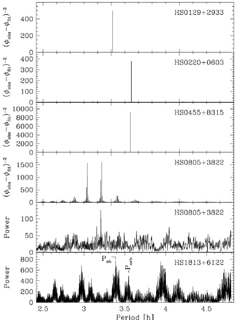
Figure 3: Time series analysis of the CCD photometry of the five new SW Sex stars. The four top panels show the results of eclipse-phase fits for the deeply eclipsing systems HS 0129+2933, HS 0220+0603, and HS 0455+8315, as well as for the grazing eclipser HS 0805+3822. For HS 0805+3822, an AOV periodogram (Schwarzenberg-Czerny, 1996) is shown in the second-lowest panel, and a Scargle (1982) periodogram is shown for HS 1813+6122 in the bottom panel, with the likely orbital period and superhump period indicated.

3.3 HS 1813+6122

The light curve of HS 1813+6122 is characterized by rapid ($10-20$ min) oscillations with a typical amplitude of $0.1-0.2$ mag, superimposed by modulations with time-scales of hours and amplitudes of $\simeq 0.1$ mag. We combined all data after subtracting the nightly means, and calculated a Scargle (1982) periodogram (Fig. 3, bottom panel). Two broad clusters of signals are found at 3.38 and 3.54 h, with the stronger signal at the shorter period. The same double-cluster structure repeats with lower amplitudes at several $\pm 1$ cycle/day aliases. Fig. 6 shows the photometric data folded on either period, after subtracting a sine fit with the respective other period.

Many of the known SW Sex stars display positive and/or negative superhumps in their light curves (e.g. Patterson & Skillman 1994; Rolfe, Haswell & Patterson 2000; Stanishev et al. 2002; Patterson et al. 2002; Patterson et al. 2005), and the pattern observed in HS 1813+6122 fits into that picture. On the basis of photometry alone, it is usually not possible to unambiguously identify orbital and superhump periods, but based on the radial velocity study described below in Sect. 4.3, we suggest that $P_{\mathrm{SH}}=3.38$ h and $\mbox{$P_{\rm orb}$}=3.54$ h.

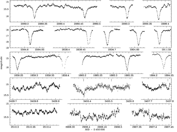
Figure 4: Sample light curves of the five new SW Sex stars. From top to bottom: HS 0129+2933, HS 0220+0603, HS 0455+8315, HS 0805+3822, and HS 1813+6122. HS 0805+3822 displays grazing eclipses. Those indicated by ticks above the light curves were used to calculate an ephemeris.

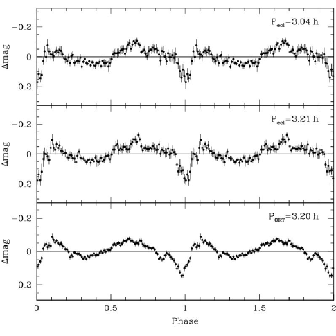
Figure 5: Phase-folded light curves of HS 0805+3822. Top and middle panels: data from the nights with low flickering activity folded over the eclipse ephemerides given by Eqs. (4,5). Bottom panel: all data folded over the period determined from an analysis-of-variance periodogram (ORT, Schwarzenberg-Czerny 1996).

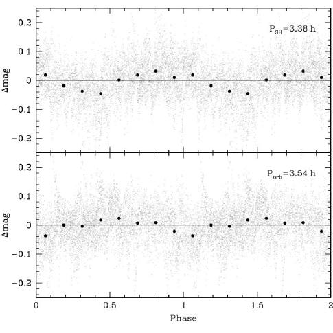
Figure 6: Phase-folded light curves of HS 1813+6122. Top panel: all data folded over $P_{\mathrm{SH}}=3.38$ h, the strongest signal detected in the periodogram (Fig. 3), after subtracting a sine fit with $P_{\mathrm{orb}}=3.54$ h, the period of the neighbouring signal. Bottom panel: all data folded over $P_{\mathrm{orb}}=3.54$ h after subtracting a sine fit with $P_{\mathrm{SH}}=3.38$ h. We interpret $P_{\mathrm{SH}}$ and $P_{\mathrm{orb}}$ as the superhump and orbital periods, respectively.

4 Spectroscopic analysis

4.1 An overabundance of nitrogen in HS 0220+0603

HS 0220+0603 shows emission lines not usually seen in CVs. In Fig. 7 we plot the average spectrum covering the region $\lambda\lambda 4870-6500$. We identify a group of lines around $\lambda$5250 as Fe ii transitions. They very likely are emission profiles plus an absorption component since a deep absorption trough is observed at the position of Fe ii $\lambda$5169. The He i $\lambda$5016 line is abnormally broad and has a strange profile with three peaks. This is probably the effect of blended He i and Fe ii emission (at $\lambda 5018$). But the most notorious feature is the broad N ii $\lambda$5680 emission. Another triple-peaked emission line profile is found at $\lambda$6350 which we identify as Si ii emission. The N ii $\lambda$5680 transition has been observed in the intermediate polar HS 0943+1404 (Rodríguez-Gil et al., 2005), and we interpret its presence as evidence of an anomalously large abundance of nitrogen.

An observed overabundance of nitrogen in the accretion flow is directly linked to the chemical abundances of the donor star, and suggests that the donor has undergone nuclear evolution via the CNO cycle. This implies that the donor had an initial mass of $\ga 1.2\,\mathrm{M}_{\odot}$ and the system evolved through a phase of thermal-time scale mass transfer (Schenker et al. 2002; Podsiadlowski, Han & Rappaport 2003). The theoretical models predict that up to 1/3 of all CVs may have undergone nuclear evolution. This seems to be confirmed by the substantial number of systems with evolved donor stars that have been found (e.g. Jameson, King & Sherrington 1980; Bonnet-Bidaud & Mouchet 1987; Thorstensen et al. 2002a, 2002b; Gänsicke et al. 2003).

4.2 Radial velocities

Radial velocity curves of the ${\mathrm{H}\alpha}$ and He ii $\lambda$4686 emission lines were computed for the eclipsing systems, except for HS 0129+2933 where He ii $\lambda$4686 is too weak and only ${\mathrm{H}\alpha}$ was measured. The individual velocity points were obtained by cross-correlating the individual profiles with single Gaussian templates matching the FWHMs of the respective average line profiles (see Table 1). Before measuring the velocities, the normalised spectra were re-binned to a uniform velocity scale centred on the rest wavelength of each line. The radial velocity curves of the three deeply-eclipsing systems folded on their respective orbital periods are presented in Fig. 8.

We fitted sinusoidal functions of the form:

$$V_{\mathrm{r}}=\gamma-K\sin\left[2\pi\left(\varphi-\varphi_{0}\right)\right]$$

to the radial velocity curves. The fitting parameters are shown in Table 5. Note that the $\gamma$ and $K$ parameters given in the table are not the actual systemic velocity and radial velocity amplitude of the white dwarf ($K_{1}$). The ${\mathrm{H}\alpha}$ line in HS 0129+2933, HS 0220+0603, and HS 0455+8315 is delayed with respect to the motion of the white dwarf by $\varphi_{0}\sim 0.2$. The He ii $\lambda$4686 radial velocity curves of HS 0220+0603 and HS 0455+8315 show the same phase offset. This phase lag indicates that the main emission site is at an angle ($\sim 72\degr$) to the line of centres between the centre of mass of the binary and the white dwarf. The radial velocity curves are not sinusoidal in shape, showing significant distortion mainly at phases 0 (mid-eclipse) and 0.5. The spikes at $\varphi\sim 0$ are due to a rotational disturbance, caused by the fact that the secondary first occults the disc material approaching us and then the receding material. This translates into a red velocity spike before mid-eclipse and a blue spike after it.

Table 5: Radial velocity curves fitting parameters.

Line	$\gamma$ ($\mathrm{km~{}s^{-1}}$)	$K$ ($\mathrm{km~{}s^{-1}}$)	$\varphi_{0}$
HS 0129+2933
${\mathrm{H}\alpha}$	$69\pm 1$	$282\pm 1$	$0.240\pm 0.001$
HS 0220+0603
${\mathrm{H}\alpha}$	$-37.0\pm 0.7$	$186\pm 1$	$0.170\pm 0.001$
He II $\lambda$4686	$-88\pm 16$	$295\pm 22$	$0.24\pm 0.01$
HS 0455+8513
${\mathrm{H}\alpha}$	$-27\pm 1$	$238\pm 1$	$0.155\pm 0.001$
He II $\lambda$4686	$5\pm 1$	$125\pm 7$	$0.14\pm 0.01$

Figure 7: Orbitally-averaged spectrum of HS 0220+0603. Notice the unusual N ii $\lambda$5680 emission line.

Figure 8: Radial velocity curves of the deeply-eclipsing systems HS 0129+2933, HS 0220+0603, and HS 0455+8315 folded on their respective orbital periods after averaging the data into 20 phase bins. The ${\mathrm{H}\alpha}$ velocities are delayed by $\sim 0.1-0.2$ orbital cycle with respect to the photometric ephemerides. The same is observed for the He ii $\lambda$4686 lines in HS 0220+0603 and HS 0455+8315. The orbital cycle has been plotted twice.

4.3 The orbital period of HS 1813+6122

Of the five new CVs, HS 1813+6122 is the only one not showing eclipses, but the photometry suggests a possible orbital period of 3.54 h (Sect. 3.3). In an attempt to confirm this value we performed a period analysis on the ${\mathrm{H}\alpha}$ and ${\mathrm{H}\beta}$ radial velocities. The velocities were derived by using the double Gaussian method of Schneider & Young (1980) (which gave better results than the single Gaussian technique), adopting a Gaussian FWHM of 200 $\mathrm{km~{}s^{-1}}$ and a separation of 1600 $\mathrm{km~{}s^{-1}}$. The 2002 September 1 and 2003 May INT data were obtained under poor observing conditions and were therefore excluded from the analysis. In Fig. 9 we show the resulting analysis-of-variance periodogram computed from the combined ${\mathrm{H}\alpha}$ and ${\mathrm{H}\beta}$ radial velocity curves. The periodogram shows its strongest peak at a period of 3.53 h, which confirms the value given by the photometric data as well as the presence of a negative superhump in the light curve of HS 1813+6122. A sine fit to the longest spectroscopic run (2003 Jun 29) with the period fixed at the above value yielded a tentative zero-phase time of $T_{0}(\mathrm{HJD})=2\,452\,819.597(2)$. A preliminary trailed spectrum revealed the characteristic SW Sex high-velocity S-wave reaching its maximum blue velocity at relative phase $\sim 0.3$ (the phases are defined by using the above $T_{0}$). By analogy with the eclipsing systems presented in this paper (Sect. 4.4), and with the eclipsing SW Sex stars in general (see e.g. Hellier, 1996; Hoard & Szkody, 1997; Hellier, 2000; Rodríguez-Gil et al., 2001), this is expected to happen at absolute phase $\varphi\sim 0.5$. Therefore, the Balmer radial velocities of HS 1813+6122 are delayed by $\varphi_{0}\sim 0.2$ with respect to the white dwarf motion, a defining characteristic of the SW Sex stars. Correcting for this we get a new time of zero phase of $T_{0}(\mathrm{HJD})=2\,452\,819.568(2)$. Fig. 9 shows the combined ${\mathrm{H}\alpha}$ and ${\mathrm{H}\beta}$ velocities folded on the orbital period with the new phase definition.

Figure 9: Top: Scargle periodogram of the ${\mathrm{H}\alpha}$+${\mathrm{H}\beta}$ radial velocity curves of HS 1813+6122. Bottom: phase folded radial velocity curve (no phase binning applied). See text for details on the adopted $T_{0}$. A full cycle has been repeated.

4.4 Trailed spectra

Trailed spectrograms of several emission lines of HS 0129+2933, HS 0220+0603, and HS 0455+8315 were constructed after re-binning the spectra on to an uniform velocity scale centred on the rest wavelength of each line. They are shown in Fig. 10. The ${\mathrm{H}\alpha}$ and ${\mathrm{H}\beta}$ line emission is dominated by a high-velocity emission component which neither follows the phasing of the primary nor the secondary. These S-waves reach their bluest velocity at $\varphi\sim 0.5$ in the three eclipsing systems and have a velocity amplitude of $\ga 600~{}\mbox{$\mathrm{km~{}s^{-1}}$}$. Weaker emission can also be seen underneath the dominant S-wave, possibly originating in the accretion disc. An absorption component is observed moving across the lines from red to blue, reaching maximum strength also at $\varphi\sim 0.5$.

The He i lines also display this high-velocity S-wave with the same phasing as the Balmer lines, as well as the absorption component. The He i $\lambda$4472 line in HS 0220+0603 shows it for approximately three quarters of an orbit, going well below the continuum.

Only HS 0220+0603 and HS 0455+8315 have a He ii $\lambda$4686 line strong enough to produce a clear trailed spectrogram. While in the former the emission seems to be entirely dominated by the high-velocity component, two components are observed in the latter: a low-velocity one (the strongest), and a weaker component which is probably the same S-wave we observe in the Balmer and He i lines. No significant absorption is detected in He ii $\lambda$4686.

In Fig. 11 we present the ${\mathrm{H}\alpha}$ trailed spectrum of HS 1813+6122 after averaging the individual spectra into 20 orbital phase bins. The line shows a high-velocity S-wave with maximum blue velocity at $\sim-2000$ $\mathrm{km~{}s^{-1}}$.

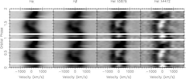
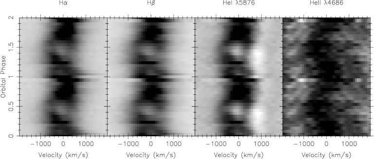
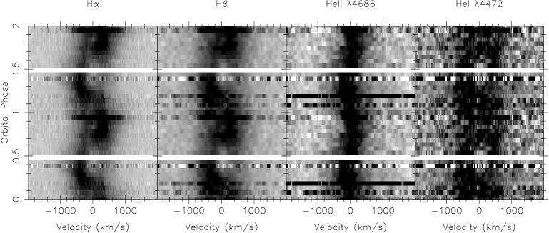
Figure 10: Trailed spectra of (from top to bottom) HS 0129+2933, HS 0220+0603, and HS 0455+8513. The individual spectra were averaged into 20 phase bins. Black represents emission. Unsampled phase bins are indicated by a blank spectrum. A full orbital cycle has been repeated for continuity.

4.5 The FUV spectrum of HS 0455+8315

The ultraviolet spectrum of HS 0455+8315 (obtained at $\varphi\simeq 0.75$) displays very strong emission lines of He, C, N, O, and Si, with line flux ratios compatible with those observed in the majority of CVs (Mauche, Lee & Kallman 1997), indicating normal chemical abundances of the donor star. The slope of the FUV continuum is nearly flat as observed in a number of deeply eclipsing SW Sex stars (e.g. DW UMa, Szkody 1987; Knigge et al. 2004; PX And, Thorstensen et al. 1991; BH Lyn, Hoard & Szkody 1997), . It has been argued that a relatively cold structure shields the inner disc and the white dwarf from view in high-inclination SW Sex stars during the high state, specifically supported by the FUV detection of the hot white dwarf in DW UMa during a low state (Knigge et al., 2000; Araujo-Betancor et al., 2003).

5 SW Sex membership

The five new CVs presented in this paper have very much in common. In their average spectra the Balmer and He i lines display both single- or double-peaked profiles. The double-peaked profiles are likely a consequence of phase-dependent absorption components as the trailed spectra show. The lines are also characterised by highly asymmetric profiles with enhanced wings. The trailed spectra reveal the presence of a high-velocity emission S-wave in all the systems with extended wings reaching a maximum velocity between $\sim\pm 2000$ $\mathrm{km~{}s^{-1}}$ (HS 1813+6122) and $\sim\pm 1000$ $\mathrm{km~{}s^{-1}}$ in the eclipsing systems. The tendency of non-eclipsing SW Sex stars to show broader S-waves may be evidence of emitting material with a vertical velocity gradient such as a mass outflow.

The radial velocity curves also show a distinctive SW Sex feature. They are delayed with respect to the motion of the white dwarf, so that the red-to-blue crossing takes place at $\varphi\sim 0.2$ instead of $\varphi=0$. On the other hand, the eclipsing systems also display a discontinuity around mid-eclipse, probably a rotational disturbance, which indicates that part of the line emission comes from the accretion disc.

All the features described above are defining characteristics of the SW Sex stars (see Thorstensen et al. 1991 and Rodríguez-Gil, Schmidtobreick & Gänsicke 2007). Even though each system exhibits its own peculiarities (e.g. unusual spectral lines in HS 0220+0603 and strong He ii $\lambda$4686 emission in HS 0455+8315), they all share the characteristic SW Sex behaviour. We therefore classify them all as new SW Sex stars.

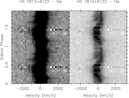
Figure 11: ${\mathrm{H}\alpha}$ trailed spectra of HS 1813+6122. Black represents emission. The grey scale has been adjusted to enhance the high-velocity S-wave (left) and the line core (right). A whole cycle has been repeated.

Figure 12: HST/STIS far-ultraviolet spectrum of HS 0455+8315.

6 The SW Sex stars in the context of CV evolution

6.1 How are the SW Sex stars discovered as CVs?

CVs are found by a number of means. Many of them display abrupt brightenings as a result of a dwarf nova eruption or a nova explosion. They also show a rich variety of photometric variations like eclipses, orbital modulations, rapid oscillations, ellipsoidal modulations, etc. Others have been discovered by their blue colour, the emission of X-rays, or the presence of strong emission lines in their optical spectra.

The total number of definite members of the SW Sex class so far known amounts to 35, out of which a remarkable number of 18 (51 per cent) has been found in UV-excess surveys (i.e. blue colour). This is not surprising, as the optical spectra of the SW Sex stars in the high-state is characterised by a very blue continuum. On the other hand, 11 SW Sex stars (31 per cent) have been identified as CVs from their emission line spectra, five of which were discovered in the HQS. Only four and two SW Sex stars have been found because of their brightness variability (including 3 novae) and X-ray emission, respectively.

Any sort of CV search has its own selection effects, and the classification of a CV as a SW Sex star is no exception. In fact, the deep eclipses that many of the SW Sex stars show initially made the sample clearly biased towards high inclination systems. This led many authors to link the SW Sex phenomenon to a mere inclination effect. At the last count, 13 out of a total of 35 SW Sex stars (37 per cent) do not display eclipses and are bona fide members of the class. Although an inclination effect may certainly be important (see the case of HL Aqr in Rodríguez-Gil et al. 2007), the increasing number of non-eclipsing systems poses serious difficulties to any model resting solely on a high orbital inclination.

In the following section we discuss on the impact of SW Sex stars in the (spectroscopic) HQS sample, which is unaffected by the high-inclination selection effect.

6.2 The role of the SW Sex stars in the big family of nova-like CVs

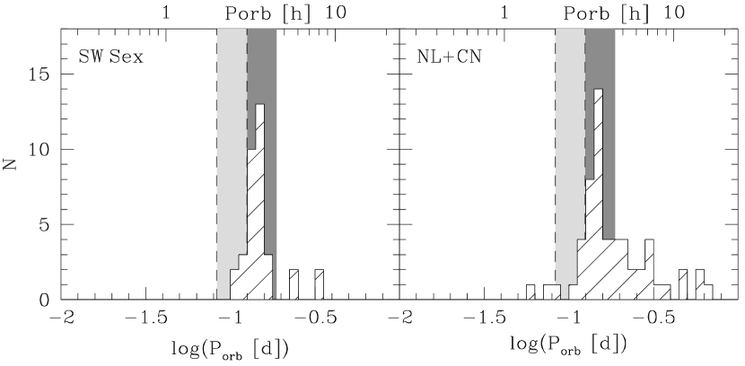
Figure 13: Period distributions of confirmed SW Sex stars (left panel) and nova-like variables and classical novae that are not known to exhibit SW Sex behaviour. The orbital period gap and the 3–4 h orbital period range are indicated in light and dark grey, respectively.

Table 6: The SW Sex stars.

Object	$P_{\mathrm{orb}}$ (h)	Eclipses	References
V348 Pup	2.44	Yes	1
V795 Her	2.60	No	2
RX J1643.7+3402	2.89	No	3
V442 Oph	2.98	No	4
AH Men	3.05	No	5
HS 0728+6738	3.21	Yes	6
HS 0805+3822	3.21	Grazing	7,
			this paper
SW Sex	3.24	Yes	8
HL Aqr	3.25	No	5
DW UMa	3.28	Yes	8
SDSS J132723.39+652854.2	3.28	Yes	9
WX Ari	3.34	Grazing	10
HS 0129+2933	3.35	Yes	This paper
V1315 Aql	3.35	Yes	8
BO Cet	3.36	No	5
AH Pic	3.41	No	5
VZ Scl	3.47	Yes	11
LN UMa	3.47	No	5
RR Pic	3.48	Grazing	12
PX And	3.51	Yes	8
V533 Her	3.53	No	13
HS 1813+6122	3.54	No	This paper
HS 0455+8315	3.57	Yes	This paper
HS 0220+0603	3.58	Yes	This paper
HS 0357+0614	3.59	No	14
V380 Oph	3.70	No	5
BH Lyn	3.74	Yes	15
UU Aqr	3.93	Yes	16
LX Ser	3.95	Yes	17
V1776 Cyg	3.95	Yes	18
LS Peg	4.19	No	19
V347 Pup	5.57	Yes	20
RW Tri	5.57	Yes	21
V363 Aur	7.71	Yes	22
BT Mon	8.01	Yes	23

References: 1 Rodríguez-Gil et al. (2001); 2 Casares et al. (1996); 3 Mickaelian et al. (2002); 4 Hoard et al. (2000); 5 Rodríguez-Gil et al. (2007); 6 Rodríguez-Gil et al. (2004); 7 Szkody et al. (2003); 8 Thorstensen et al. (1991); 9 Wolfe et al. (2003); 10 Beuermann et al. (1992); 11 Moustakas & Schlegel (1999); 12 Schmidtobreick, Tappert & Saviane (2003); 13 Rodríguez-Gil & Martínez-Pais (2002); 14 Szkody et al. (2001); 15 Thorstensen, Davis & Ringwald (1991); 16 Hoard et al. (1998); 17 Young, Schneider & Shectman (1981); 18 Garnavich et al. (1990); 19 Taylor et al. (1999); 20 Thoroughgood et al. (2005); 21 Groot, Rutten & van Paradijs (2004); 22 Thoroughgood et al. (2004); 23 Smith, Dhillon & Marsh (1998)

In Table 6 we list the 35 known SW Sex stars along with their orbital periods. Before doing any statistics we want to stress the fact that Table 6 does not intend to present a definitive census of the SW Sex stars. This is because their defining characteristics are continuously evolving as we dig deeper into the understanding of this class of CVs. For comparison (and probably completeness) we also point the reader to Don Hoard’s Big List of SW Sex stars.

Table 6 shows that a significant 37 per cent of the family does not show eclipses, confirming that the high inclination requirement is merely a selection effect. The orbital period distribution of the known sample of SW Sex stars is presented in the left panel of Fig. 13. The combined distributions for non-SW Sex nova-likes and nova remnants are also plotted for comparison. The nova-likes and novae were selected from the Ritter (Ritter & Kolb, 2003), CVcat (Kube et al., 2003), and Downes (Downes et al., 2005) catalogues. Only systems with a robust orbital period determination are included.

These orbital period distributions reveal important features. About 40 per cent (35 out of 93) of the whole nova-like/classical nova population (which is preferentially found above the period gap; only 12 are below it) are indeed SW Sex stars. Even more remarkable is the fact that the SW Sex stars represent almost half (26 out of 53) the CVs in the narrow $3-4.5$ h orbital period range. Above 4.5 h things radically change and only 14 per cent (4 out of 28) of the nova-like/nova population are known to be SW Sex stars. The impact of SW Sex stars in the gap is also striking, as 55 per cent of all the nova-like/nova gap inhabitants are members of the class.

The non-SW Sex nova-like/nova $P_{\mathrm{orb}}$ distribution also shows a significant fraction of systems in the $3-4.5$ h interval. This nicely depicts the tendency of nova-likes to accumulate in the $3-4.5$ h period range. Therefore, it is very likely that more SW Sex stars are still to be found. In fact, time-resolved spectroscopic studies like the one reported in Rodríguez-Gil et al. (2007) are revealing the SW Sex nature of many previously poorly studied nova-likes in this range. If the rate of detection and identification of SW Sex systems remains high the dominance of this class at the upper edge of the gap will eventually become even more pronounced.

It is possible, however, that these numbers are the result of a selection effect as the majority of SW Sex stars are bright, making them easily accesible to observations. Therefore, one can argue that a proper characterisation of the whole population of CVs above the gap needs to be made before addressing any conclusion. However, the fact the majority of SW Sex stars have orbital periods between 3 and 4.5 h is a well established fact.

6.2.1 The impact of SW Sex stars on the HQS CV sample

During the course of our spectroscopic search we have discovered 53 new CVs in the area/magnitude range covered by the HQS ($\simeq 13600$ square degrees/$17.5\la B\la 18.5$; see Hagen et al. 1995). So far, we have determined the orbital period for 43 of them in a huge observational effort. Our preliminary results support the SW Sex excess within the $3-4.5$ h range. Remarkably, 54 per cent (7 out of 13) of all the newly-discovered HQS nova-likes are indeed SW Sex stars, which is in agreement with the distribution discussed above. This gives further strength to the significancy of the observed (and still unexplained) pile-up of SW Sex stars in the $3-4.5$ h region.

6.3 CV evolution and the SW Sex stars

This accumulation of systems just above the period gap seriously challenges our current understanding of CV evolution. The SW Sex stars are intrinsically very luminous, as the brightness of systems like DW UMa indicates. DW UMa is a SW Sex star likely located at a distance between $\sim 590-930$ pc (Araujo-Betancor et al., 2003) that has an average magnitude of $V\sim 14.5$, even though it is viewed at an orbital inclination of $\sim 82$°. Therefore, in order to show such high luminosities, either the SW Sex stars have an average mass transfer rate well above that of their CV cousins, or another source of luminosity exists. Neither the Rappaport, Joss & Verbunt (1983) nor the (empirical) Sills, Pinsonneault & Terndrup (2000) angular momentum loss prescriptions account for a largely enhanced mass transfer rate ($\dot{M}$) in the period interval where most of the SW Sex stars reside. In this regard, nuclear burning has been suggested as an extra luminosity source (Honeycutt, 2001), but the necessary conditions for the burning to occur can only be found in the base of a magnetic accretion funnel, suggesting a magnetic nature (Honeycutt & Kafka, 2004). Temporary cessation of nuclear burning would in principle explain the VY Scl low states that many SW Sex and other nova-likes undergo. If this is true, the majority of CVs above the period gap have to be magnetic, in stark contrast with a non-magnetic majority below the gap. However, the fact that some dwarf novae (like HT Cas and RX And) also show low states (e.g. Robertson & Honeycutt 1996; Schreiber, Gänsicke & Mattei 2002) argues against this possibility, suggesting that the VY Scl states are likely the product of a decrease in the mass transfer rate from the donor star caused by starspots, as already proposed by Livio & Pringle (1994). The observational results of Honeycutt & Kafka (2004) appear to support this hypothesis (see also e.g. Howell et al., 2000).

All of the above arguments point to accretion at a very high $\dot{M}$ as the most likely cause for the high luminosity observed in the SW Sex stars. One possibility could be enhanced mass transfer due to irradiation of the inner face of the secondary star by a very hot white dwarf. In fact, a number of nova-like CVs in the $\sim 3-4$ h orbital period range (including the SW Sex star DW UMa) have been observed to harbour the hottest white dwarfs found in any CV (see Araujo-Betancor et al., 2005), with effective temperatures peaking at $\sim 50\,000$ K. These high temperatures are most likely the result of accretion heating, as CVs are thought to spend on average $\sim 2$ Gyr as detached binary systems (Schreiber & Gänsicke, 2003), enough time for the white dwarfs to cool down to $\la 8000$ K. Hence, the high effective temperatures measured in the $3-4$ h range is a measure of a very high secular mass accretion rate of $\sim 5\times 10^{-9}~{}\mathrm{M_{\odot}}\,\mathrm{yr}^{-1}$ (Townsley & Bildsten, 2003), higher than predicted by angular momentum loss due to magnetic braking. Irradiation of the donor star has been observed in the non-eclipsing SW Sex stars HL Aqr, BO Cet, and AH Pic (Rodríguez-Gil et al., 2007), which supports the above hypothesis. Alas, the question of why the SW Sex stars have the highest mass transfer rates is still lacking a satisfactory explanation in the context of the current CV evolution theory.

6.4 A rich phenomenology to explore

It is becoming apparent that the SW Sex phenomenon is not restricted to the (mainly) spectroscopic properties initially introduced by Thorstensen et al. 1991. These maverick CVs are now known to show a much more intricate behaviour. Therefore, only a comprehensive study of this rich phenomenology will definitely lead to a full understanding of the SW Sex stars. In what follows we will review the range of common features exhibited by the SW Sex stars and which implications can be derived from them.

6.4.1 Superhumps

A significant one third of the SW Sex stars is known to show apsidal (positive) or/and nodal (negative) superhumps, which are large-amplitude photometric waves modulated at a period slightly longer or slightly shorter than the orbital period, respectively. Positive superhumps are believed to be the effect of an eccentric disc which is forced to progradely precess by the tidal perturbation of the donor star (Whitehurst, 1988). On the other hand, negative superhumps are likely linked to the retrograde precession of a warped accretion disc (Murray et al., 2002). Vertical changes in the structure of the disc may be triggered by the torque exerted on the disc by the tilted, dipolar magnetic field of the secondary star. Apparently, positive and negative superhumps are independent and can either coexist or alternate with a time scale of years.

The detection of superhumps in the SW Sex stars is of great importance as they exhibit the largest superhump period excesses. Therefore, they are fundamental in calibrating the period excess–mass ratio relationship for CVs (see Patterson et al., 2005).

6.4.2 Variable eclipse depth

The continuum light curves of some eclipsing members of the class reveal that the eclipse depth varies with a time-scale of several days. So far this variability has only been studied in PX And (Stanishev et al., 2002; Boffin et al., 2003) and DW UMa (Bíró, 2000; Stanishev et al., 2004, not to be confused with the changing eclipse depth in different brightness states). In PX And, Stanishev et al. 2002 identify this long periodicity with the precession period of the accretion disc, which may also be true for DW UMa. The actual mechanism is not yet understood, although the eclipses of a retrogradely precessing, warped disc may account for what is observed in PX And (Boffin et al., 2003).

6.4.3 Low states

Half of the nova-likes known to undergo VY Scl faint states are SW Sex stars. During these events the system brightness can drop by up to $\sim 4-5$ mag and can remain that low for months. As the disc warping effect mentioned above, these low states may be controlled by the strong magnetic activity of the donor star, and are believed to be driven by a sudden drop of the accretion rate from the secondary star due to large starspots located in the area around the inner Lagrangian point $\mathrm{L}_{1}$ (Livio & Pringle, 1994).

Interestingly, the disced VY Scl stars concentrate in the $3-4.5$ h orbital period stripe as the SW Sex stars do. It would therefore not be a surprise to find that all nova-likes in that range are actually VY Scl stars and even SW Sex stars. Nevertheless, the presence of large starspots around the $\mathrm{L}_{1}$ point still have to be observationally confirmed. Using Roche tomography techniques, Watson, Dhillon & Shahbaz (2006) discovered a heavily spotted secondary star in AE Aqr ($P_{\mathrm{orb}}=9.88$ h) with a spot distribution resembling that of other rapidly rotating, low-mass field stars. A stellar atmosphere plagued with spots has been also observed in the pre–CV V471 Tau ($P_{\mathrm{orb}}=12.51$ h, Hussain et al., 2006). Unfortunately, the high spectral and time resolution required to image the M-dwarf donor in a CV with $P_{\mathrm{orb}}\simeq 3.5$ h at a distance of many hundred parsecs is currently beyond observational reach.

6.4.4 Quasi-periodic oscillations

On the grounds of short-term variability, the SW Sex stars are also characterised for exhibiting quasi-coherent modulations in their light curves. In a compilation of CVs displaying rapid oscillations, Warner (2004) lists 9 (only two deeply eclipsing) SW Sex stars known to have quasi-periodic oscillations (QPOs) with a predominant time-scale of $\sim 1000-2000$ s. For example, the non-eclipsing SW Sex stars V442 Oph and RX J1643.7+3402 show strong QPO signals dominating over other underlying higher-coherence oscillations (Patterson et al., 2002). These results are based on hundreds of hours of photometric data, whose power spectra showed rapid frequency changes of the main signals in less than a day. Similar rapid variability was also detected in the optical light curve of the SW Sex star HS 0728+6738 (Rodríguez-Gil et al., 2004), with a prominent signal (coherent for at least 20 cycles) at $\sim 600$ s.

6.4.5 Emission-line flaring

In connection with the QPO activity, the fluxes and EWs of the emission lines of some SW Sex stars show modulations at the same time-scales (a phenomenon known as emission-line flaring): $\sim 1800$ s in BT Mon (Smith et al., 1998), $\sim 2000$ s in LS Peg (Rodríguez-Gil et al., 2001), $\sim 1400$ s in V533 Her (Rodríguez-Gil & Martínez-Pais, 2002), $\sim 1800$ s in DW UMa (V. Dhillon, private communication), $\sim 2400$ s in RX J1643.7+3402 (Martínez-Pais, de la Cruz Rodríguez & Rodríguez-Gil 2007), and $\sim 1200$ s in BO Cet (Rodríguez-Gil et al., 2007). Remarkably, the radial velocities measured in the last two objects are also modulated at the flux/EW periodicities, which suggests that emission-line flaring has to do with the dynamics of the line emitting source, and is not due to e.g. random fluctuations in the disc continuum emission. On the other hand, although DW UMa does exhibit emission-line flaring in the optical, such line variability was not detected in the far ultraviolet (Hoard et al., 2003). Since similar flaring in the optical is observed in the intermediate polar CVs (IPs; e.g. FO Aqr Marsh & Duck, 1996) caused by the rotation of the magnetic white dwarf, all the described rapid variations seen in many SW Sex stars have been associated to the presence of magnetic white dwarfs (Rodríguez-Gil et al., 2001; Patterson et al., 2002). Nevertheless, the far ultraviolet data of DW UMa presented by Hoard et al. (2003) can also be explained with a stream overflow model, but do not necessary exclude a magnetic scenario either.

6.4.6 Variable circular polarisation

Despite the fact that circular polarisation is not commonly detected in the majority of IPs, it is a sine qua non condition for IP membership (see further requirements in Patterson, 1994). The cyclotron radiation emitted by the accretion columns (built up by disc plasma forced by the magnetic field to supersonically fall on to the white dwarf surface) is known to be circularly polarised, thus the detection of a significant level of circular polarisation is a unequivocal sign of magnetic accretion. This, and the possible magnetic nature of the QPO and line flaring activity prompted to the search for circular polarisation in the SW Sex stars.

Rodríguez-Gil et al. (2001) found circular polarisation modulated at 1776 s with a peak-to-peak amplitude of 0.3 per cent in LS Peg. Remarkably, the flaring observed in the ${\mathrm{H}\beta}$ high-velocity S-wave was modulated at 2010 s, which is just the synodic period between the polarisation period and the orbital period. V795 Her also revealed variable circular polarisation with a periodicity of 1170 s (or twice that) and showed an increasing polarisation level with wavelength (Rodríguez-Gil et al., 2002) as is expected for cyclotron emission. In addition, RX J1643.7+3402 shows circular polarisation modulated at 1163 s (Martínez-Pais et al., 2007).

The 1776-s period of LS Peg was confirmed by Baskill, Wheatley & Osborne (2005) who detected a coherent modulation at 1854 s in ASCA X-ray light curves. The coincidence of both periods indicates a common origin, with the X-ray period reported by Baskill et al. likely being a more accurate measurement of the white dwarf spin period.

Although polarimetric studies of many other SW Sex stars have to be done, the results obtained so far suggest that magnetic accretion may play an important role in the SW Sex phenomenon. However, with the few such studies so far at hand it is not possible to address any conclusion regarding the impact of magnetism in the whole class.

Despite the broad implications in our understanding of accretion that the study of the SW Sex stars have, the quest for a successful, global explanation of the phenomenon has been unfruitful so far. This, in addition to the (yet unexplained) fact that the majority of SW Sex stars (and many nova-likes) largely populate the narrow orbital period stripe between 3 and 4.5 hours, are seriously shaking the grounds on which CV evolution theory stands. Further study of these maverick systems will certainly provide fundamental clues to our understanding of CV evolution.

References

- Araujo-Betancor et al. (2005) Araujo-Betancor S., Gänsicke B. T., Long K. S., Beuermann K., de Martino D., Sion E. M., Szkody P., 2005, ApJ, 622, 589
- Araujo-Betancor et al. (2003) Araujo-Betancor S., et al., 2003, ApJ, 583, 437
- Aungwerojwit et al. (2005) Aungwerojwit A., et al., 2005, A&A, 443, 995
- Baskill et al. (2005) Baskill D. S., Wheatley P. J., Osborne J. P., 2005, MNRAS, 357, 626
- Bertin & Arnouts (1996) Bertin E., Arnouts S., 1996, A&AS, 117, 393
- Beuermann et al. (1992) Beuermann K., Thorstensen J. R., Schwope A. D., Ringwald F. A., Sahin H., 1992, A&A, 256, 442
- Bíró (2000) Bíró I. B., 2000, A&A, 364, 573
- Boffin et al. (2003) Boffin H. M. J., Stanishev V., Kraicheva Z., Genkov V., 2003, in Sterken C., ed, ASP Conf. Ser. Vol. 292, Interplay of Periodic, Cyclic and Stochastic Variability in Selected Areas of the H-R Diagram. Astron. Soc. Pac., San Francisco, p. 297
- Bonnet-Bidaud & Mouchet (1987) Bonnet-Bidaud J. M., Mouchet M., 1987, A&A, 188, 89
- Casares et al. (1996) Casares J., Martínez-Pais I. G., Marsh T. R., Charles P. A., Lázaro C., 1996, MNRAS, 278, 219
- Dhillon et al. (1992) Dhillon V. S., Jones D. H. P., Marsh T. R., Smith R. C., 1992, MNRAS, 258, 225
- Downes et al. (2005) Downes R. A., Webbink R. F., Shara M. M., Ritter H., Kolb U., Duerbeck H. W., 2005, VizieR Online Data Catalog, 5123
- Gänsicke et al. (2004) Gänsicke B. T., Araujo-Betancor S., Hagen H.-J., Harlaftis E. T., Kitsionas S., Dreizler S., Engels D., 2004, A&A, 418, 265
- Gänsicke et al. (2003) Gänsicke B. T., et al., 2003, ApJ, 594, 443
- Gänsicke et al. (2002) Gänsicke B. T., Hagen H. J., Engels D., 2002, in Gänsicke B. T., Beuermann K., Reinsch K., eds, ASP Conf. Ser. Vol. 261, The Physics of Cataclysmic Variables and Related Objects. Astron. Soc. Pac., San Francisco, p. 190
- Garnavich et al. (1990) Garnavich P. M., et al., 1990, ApJ, 365, 696
- Green et al. (1986) Green R. F., Schmidt M., Liebert J., 1986, ApJS, 61, 305
- Groot et al. (2004) Groot P. J., Rutten R. G. M., van Paradijs J., 2004, A&A, 417, 283
- Hagen et al. (1995) Hagen H. J., Groote D., Engels D., Reimers D., 1995, A&AS, 111, 195
- Hameury & Lasota (2002) Hameury J. M., Lasota J. P., 2002, A&A, 394, 231
- Hellier (1996) Hellier C., 1996, ApJ, 471, 949
- Hellier (2000) Hellier C., 2000, New Astronomy Reviews, 44, 131
- Hellier & Robinson (1994) Hellier C., Robinson E. L., 1994, ApJ, 431, L107
- Hoard & Szkody (1997) Hoard D. W., Szkody P., 1997, ApJ, 481, 433
- Hoard et al. (2003) Hoard D. W., Szkody P., Froning C. S., Long K. S., Knigge C., 2003, AJ, 126, 2473
- Hoard et al. (1998) Hoard D. W., Szkody P., Still M. D., Smith R. C., Buckley D. A. H., 1998, MNRAS, 294, 689
- Hoard et al. (2000) Hoard D. W., Thorstensen J. R., Szkody P., 2000, ApJ, 537, 936
- Honeycutt (2001) Honeycutt R. K., 2001, PASP, 113, 473
- Honeycutt & Kafka (2004) Honeycutt R. K., Kafka S., 2004, AJ, 128, 1279
- Horne (1986) Horne K., 1986, PASP, 98, 609
- Horne (1999) Horne K., 1999, in Hellier C., Mukai K., eds, ASP Conf. Ser. Vol. 157, Annapolis Workshop on Magnetic Cataclysmic Variables. Astron. Soc. Pac., San Francisco, p. 349
- Howell et al. (2000) Howell S. B., Ciardi D. R., Dhillon V. S., Skidmore W., 2000, ApJ, 530, 904
- Hussain et al. (2006) Hussain G. A. J., Allende Prieto C., Saar S. H., Still M., 2006, MNRAS, 367, 1699
- Jameson et al. (1980) Jameson R. F., King A. R., Sherrington M. R., 1980, MNRAS, 191, 559
- Knigge et al. (2004) Knigge C., Araujo-Betancor S., Gänsicke B. T., Long K. S., Szkody P., Hoard D. W., Hynes R. I., Dhillon V. S., 2004, ApJ, 615, L129
- Knigge et al. (2000) Knigge C., Long K. S., Hoard D. W., Szkody P., Dhillon V. S., 2000, ApJ, 539, L49
- Kube et al. (2003) Kube J., Gänsicke B. T., Euchner F., Hoffmann B., 2003, A&A, 404, 1159
- Livio & Pringle (1994) Livio M., Pringle J. E., 1994, ApJ, 427, 956
- Marsh & Duck (1996) Marsh T. R., Duck S. R., 1996, New Astronomy, 1, 97
- Martínez-Pais et al. (2007) Martínez-Pais I. G., de la Cruz Rodríguez J., Rodríguez-Gil P., 2007, MNRAS, submitted
- Martínez-Pais et al. (1999) Martínez-Pais I. G., Rodríguez-Gil P., Casares J., 1999, MNRAS, 305, 661
- Mauche et al. (1997) Mauche C. W., Lee Y. P., Kallman T. R., 1997, ApJ, 477, 832
- Mickaelian et al. (2002) Mickaelian A. M., Balayan S. K., Ilovaisky S. A., Chevalier C., Véron-Cetty M.-P., Véron P., 2002, A&A, 381, 894
- Monet et al. (2003) Monet et al. D. G., 2003, AJ, 125, 984
- Moustakas & Schlegel (1999) Moustakas J., Schlegel E. M., 1999, BAAS, 31, 1421
- Murray et al. (2002) Murray J. R., Chakrabarty D., Wynn G. A., Kramer L., 2002, MNRAS, 335, 247
- Patterson (1994) Patterson J., 1994, PASP, 106, 209
- Patterson et al. (2002) Patterson J., et al., 2002, PASP, 114, 1364
- Patterson et al. (2005) Patterson J., et al., 2005, PASP, 117, 1204
- Patterson & Skillman (1994) Patterson J., Skillman D. R., 1994, PASP, 106, 1141
- Penning et al. (1984) Penning W. R., Ferguson D. H., McGraw J. T., Liebert J., Green R. F., 1984, ApJ, 276, 233
- Podsiadlowski et al. (2003) Podsiadlowski P., Han Z., Rappaport S., 2003, MNRAS, 340, 1214
- Rappaport et al. (1983) Rappaport S., Joss P. C., Verbunt F., 1983, ApJ, 275, 713
- Ritter & Kolb (2003) Ritter H., Kolb U., 2003, A&A, 404, 301
- Robertson & Honeycutt (1996) Robertson J. W., Honeycutt R. K., 1996, AJ, 112, 2248
- Rodríguez-Gil (2005) Rodríguez-Gil P., 2005, in Hameury J.-M., Lasota J.-P., eds, ASP Conf. Ser. Vol. 330, The Astrophysics of Cataclysmic Variables and Related Objects. Astron. Soc. Pac., San Francisco, p. 335
- Rodríguez-Gil et al. (2000) Rodríguez-Gil P., Casares J., Dhillon V. S., Martínez-Pais I. G., 2000, A&A, 355, 181