Inflation, bifurcations of nonlinear curvature Lagrangians and dark energy

A possible equivalence of scalar dark matter, the inflaton, and modified gravity is analyzed. After a conformal mapping, the dependence of the effective Lagrangian on the curvature is not only singular but also bifurcates into several almost Einsteinian spaces, distinguished only by a different effective gravitational strength and cosmological constant. A swallow tail catastrophe in the bifurcation set indicates the possibility for the coexistence of different Einsteinian domains in our Universe. This ‘triple unification’ may shed new light on the nature and large scale distribution not only of dark matter but also on ‘dark energy’, regarded as an effective cosmological constant, and inflation.

1 Introduction

The origin of the principal constituents of the Universe in the form of dark matter (DM) and dark energy (DE) (or rather dark tension due to its negative pressure), remains a major puzzle of modern cosmology and particle physics. Ad hoc proposals like modifying Newton’s law of gravity as in Milgrom’s MOND (Modified Newtonian Dynamics) are difficult to reconcile with relativity, or need a phase coupling to a complex scalar [4]. The particle physics’ view is to leave gravity untouched but postulate WIMPs (Weakly Interacting Massive Particles) like axions, dilatons or neutralinos as dark matter candidates [67].

The dominant non-visible “dark” fraction of the total energy of the Universe is known to exist from its gravitational effects. Since the dark matter part is distributed over rather large distances, its interaction, including a possible self-interaction [61], must be weak. The main candidates for such weakly interacting particles are the (universal) axion or the lightest supersymmetric particle, as the neutralino in most models, cf. Ref. [67].

Recently, an observed excess of diffuse gamma rays has been attributed [9] to the annihilation of DM in our Galaxy. The flux of the presumed neutralino annihilation allows a reconstruction of the distribution of DM in our Galaxy. Most probable is a pseudo-isothermal profile but with a substructure of two doughnut-shape rings in the galactic plane. It is believed that these transient substructures have their origin in the hierarchical clustering of DM into galaxies. However, there are reservations concerning the internal consistency in the interpretation of the observations: Given the same normalization for the cross section of the DM particle, it appears unlikely [2] that DM annihilation is the main source of the extragalactic gamma-ray background (EGB). Moreover, then the large accompanied antiproton flux needs to meet several constraints [6].

On the other hand, heterotic string theory provides a very light universal axion which may avoid [13] the strong $CP$ problem in quantum chromodynamics (QCD) [51]. Given the existence of such almost massless (pseudo-)scalars, it has been speculated that a coherent non-topological soliton (NTS) type solution of a nonlinear Klein-Gordon equation can account for the observed halo structure, simulating a Bose-Einstein condensate of astronomical size [17, 18, 35]; cf. Ref. [54]. In particular, a $\Phi^{6}$ toy model [44] yields exact Emden type solutions in flat spacetime, including a flattening [38] of halos with ellipticity $e<1$ as observed via microlensing [15, 55].

Both views are to some extend physically equivalent, i.e., scalar dark matter minimally coupled to Einstein’s general relativity (GR) is equivalent [28, 5, 60, 56, 50] to a modified gravity in the relativistic framework of higher-order curvature Lagrangians. Such effective Lagrangians may also arise from the low-energy limit of (super-) strings. The model proposed by Carroll et al. [7] also uses such an equivalence of a nonlinear higher-order curvature Lagrangian, in order to explain the present cosmic acceleration, but takes resort to an $1/R$ type curvature Lagrangian, which is unbounded for weak gravitational fields.

Quite generally, the dependence of the effective Lagrangian $L$ on the scalar curvature $R$ is singular and cannot always be represented analytically in the $(R,L)$ plane. More stunning is our recent finding [56] that, although nonlinear, a $L=L(R)$ type Lagrangian bifurcates in several branches of almost linear Lagrangians

$$L\simeq\frac{1}{2\kappa_{\rm eff}}\left(R-2\Lambda_{\rm eff}\right)$$ (1)

distinguished only by the effective gravitational constant $\kappa_{\rm eff}$ and a cosmological constant $\Lambda_{\rm eff}$.

This indicates a unifying picture of dark matter, ‘dark energy’[54] with an equation of state parameter $w_{\rm DE}=p/\rho\simeq-1$, and modified gravity which may account, on different scales, for inflation [41, 38], dark matter halos [44, 37] of galaxies or even dark matter condensations, the so-called boson stars [24, 25, 42, 59] as candidates of MACHOs (Massive Compact Halo Objects). The ‘landscape’ view [26] of (super-)strings suggests also such a triple unification based on coherent, possibly oscillating scalar field with a mass larger than the Hubble scale at the present epoch, i.e. $m>H_{*}=10^{-23}$ eV.

2 Gravitationally coupled scalar fields

Conventionally, dark matter and inflation can be modeled by a real (or complex) scalar field $\phi$ with self-interaction $U(|\phi|^{2})$ minimally coupled to gravity with the Lagrangian density

$${\mathcal{L}}_{\rm DM}=\frac{\sqrt{\mid g\mid}}{2\kappa}\left\{R+\kappa\Bigl{[}g^{\mu\nu}(\partial_{\mu}\phi^{*})(\partial_{\nu}\phi)-2U(|\phi|^{2})\right]\Bigr{\}}\,,$$ (2)

where $\kappa=8\pi G$ is the gravitational constant in natural units, $g$ the determinant of the metric $g_{\mu\nu}$, and $R$ the scalar curvature of Riemannian spacetime with Tolman’s sign conventions [64]. A constant potential $U_{0}=\Lambda/\kappa$ would simulate the cosmological constant $\Lambda$.

In a wide range of inflationary models, the underlying dynamics is simply that of a single scalar field — the inflaton — rolling in some underlying potential. This scenario invented by Linde [27] is generically referred to as chaotic inflation due to its choice of initial conditions. Many superficially more complicated models can also be rewritten in this framework.

3 General metric of a flat inflationary universe

A spatially flat ($k=0$) Friedman-Robertson-Walker (FRW) Universe with metric

$$ds^{2}=dt^{2}-a^{2}(t)\left[dr^{2}+r^{2}\left(d\theta^{2}+\sin^{2}\theta d\varphi^{2}\right)\right]\;$$ (3)

is nowadays favored by observations [62]. Its temporal evolution of the generic model (2) is determined by the two autonomous first order equations

$$\dot{H} = -3H^{2}(1+w_{\rm DE})=\kappa U(\phi)-3H^{2}=:V(H,\phi)\;,$$ (4)

$$\dot{\phi} = \pm\sqrt{\frac{2}{\kappa}}\sqrt{3H^{2}-\kappa U(\phi)}=\pm\sqrt{-\frac{2}{\kappa}V(H,\phi)}\;,$$ (5)

where $H=\dot{a}(t)/a(t)$ is the Hubble expansion rate.

The function $V(H,\phi)$ will turn to be the “height function” in Morse theory [47]. Observe that $V\leq 0$ in order to avoid scalar ghosts. For the FRW metric, the Lagrangian density (2) reduces to

$${\mathcal{L}}=-\frac{3}{\kappa}\dot{a}^{2}a+\left[\frac{1}{2}\dot{\phi}^{2}-U(\phi)\right]a^{3}\;.$$ (6)

Since the shift function is normalized to one for the FRW metric, the canonical momenta are given by $P=\partial{\mathcal{L}}/\partial\dot{a}=-6Ha^{2}/\kappa$ and $\pi=\partial{\mathcal{L}}/\partial\dot{\phi}=a^{3}\dot{\phi}$. The Hamiltonian or “energy function” is given by

$$E=\Biggl{[}\frac{1}{2}\dot{\phi}^{2}+\frac{1}{\kappa}V(H,\phi)\Biggr{]}\,a^{3}\cong 0$$ (7)

and, due to (5), vanishes for all solutions, which is a familiar constraint in GR.

Using the Hubble expansion rate $H:=\dot{a}(t)/a(t)$ as the new “inverse time” coordinate

$$t=t(H)=\int\frac{dH}{\kappa\widetilde{U}-3H^{2}}\,,$$ (8)

we were able to find the general solution [57]:

$$a = a(H)=a_{0}\exp\left(\int\frac{HdH}{\kappa\widetilde{U}-3H^{2}}\right)\;.$$ (9)

$$ds^{2} = \frac{dH^{2}}{\left(\kappa\widetilde{U}-3H^{2}\right)^{2}}-a_{0}{}^{2}\exp\left(2\int\frac{HdH}{\kappa\widetilde{U}-3H^{2}}\right)\times$$ (10)

$$\left[dr^{2}+r^{2}\left(d\theta^{2}+\sin^{2}\theta d\varphi^{2}\right)\right]\;,$$

$$\phi = \phi(H)=\mp\sqrt{\frac{2}{\kappa}}\int\frac{dH}{\sqrt{3H^{2}-\kappa\widetilde{U}}}\;,$$ (11)

where $\widetilde{U}=\widetilde{U}(H):=U(\phi(t(H)))$ is the reparametrized inflationary potential.

The singular case $\widetilde{U}=3H^{2}/\kappa$ with $w_{\rm DE}=-1$ leads in (4) to the de Sitter inflation with exponential expansion $a(t)=a_{0}\exp(\sqrt{\Lambda/3\,}t)$, which for a later time becomes physically unrealistic, since the inflationary expansion eventually needs to merge into the usual Friedman cosmos. Therefore, in explicit models we use the ansatz

$$\widetilde{U}(H)=\frac{3}{\kappa}H^{2}+\frac{g(H)}{\kappa}\,,$$ (12)

for the potential, where $g(H)=V\left(H,\phi(t(h))\right)$ is a nonzero function which should provide the graceful exit from the inflationary phase to the Friedman cosmos. In order to have a positive acceleration during the inflationary phase, but on the other hand a real scalar field in (11), its allowed range is $-H^{2}<g<0$. This $H$–formalism facilitates considerably the reconstruction of the inflaton potential [57, 41, 37]. In second order this is based on an Abel equation [14] for the primordial density $\epsilon=-g/H^{2}$.

3.1 Classification by catastrophe theory

A general classification of all allowed inflationary potentials and scenarios has already been achieved by Kusmartsev et al. [23] via the application of catastrophe theory to the Hamilton–Jacobi type equations (4) and (5) regarded as an autonomous nonlinear system.

In phase space, the equilibrium states are given by the constraint $\{\dot{H},\dot{\phi}\}=0$. The critical or equilibrium points, respectively, of this system are determined by $V(H_{c},\phi_{c})=0$. This constraint is globally fulfilled by $\kappa U(\phi)=3H_{\Lambda}^{2}$, where the Hubble expansion rate is constant, i.e. $H_{\Lambda}=:\sqrt{\Lambda/3}$ corresponding to $w_{\rm DE}=-1$. For $\dot{\phi}=0$ and $\Lambda\neq 0$, we recover the de Sitter inflation.

In general, the Jacobi matrix

$$J=\left(\begin{array}[]{cc}-6H&\qquad\kappa U^{\prime}\\ \pm 6H(-2\kappa V)^{-1/2}&\qquad\mp\kappa U^{\prime}(-2\kappa V)^{-1/2}\end{array}\right)\;,$$ (13)

of the system (4) and (5) depends crucially on $U^{\prime}=dU/d\phi$. Since its determinant vanishes, i.e. $\det J=0$, the system is always degenerate. For the analysis of stability, it suffices therefore to consider only (4) and to reconstruct $\phi$ later. Since $H$ and $\phi$ are independent variables, we can introduce the non–Morse superpotential $W(H,\phi)$, defined via $V:=-\partial W/\partial H$, and analyze the system with the aid of catastrophe theory. From (4) we obtain

$$W(H,\phi)=H^{3}-\kappa U(\phi)H+C(\phi)\;,$$ (14)

where $C$ is an arbitrary function of $\phi$. The function $W$ is already in canonical form in $H$–space, and belongs to a Whitney surface[3, 22] or to the Arnold singularity class $A_{2}$. The corresponding Whitney surface has only one control parameter, the potential $U$. Thus, an evolution of critical points is determined via the values of the potential $U$. Let us analyze the types of critical points at different fixed values of the control parameter $U$.

If $U_{c}:=U(\phi_{c})<0$, the equation has no stable critical point due to the shape of the Whitney surface. However if $U_{c}>0$, there are two critical points: a stable one at $H_{c}=\sqrt{U_{c}/3}$ and an unstable one at $H_{c}=-\sqrt{U_{c}/3}$.

The value $U_{c}=0$ is the bifurcation point. Provided this is also an extremal of $V$, we necessarily have $\partial V/\partial H\mid_{c}=-6H_{c}=0$, $\partial V/\partial\phi\mid_{c}=\kappa U^{\prime}_{c}=0$, and $\dot{\phi}_{c}=0$. Thus, also the critical points of the Klein–Gordon equation for the scalar field are involved. Hence, the Hubble parameter has to vanish and $\phi_{c}$ is a double zero of the potential $U$. The Hessian of (4) takes the form

$${\rm Hess}(V)=\left(\begin{array}[]{cc}-6&0\\ 0&\kappa U^{\prime\prime}\end{array}\right)\;.$$ (15)

The sub–determinants of the Hessian are $\Delta_{0}=\partial^{2}V/\partial H^{2}=-6<0$ and $\Delta_{1}=\det{\rm Hess}(V)=(\partial^{2}V/\partial H^{2})\;(\partial^{2}V/\partial\phi^{2})-(\partial^{2}V/(\partial H\partial\phi))^{2}=-6\kappa U^{\prime\prime}$. For a maximum of the potential $U$, i.e. $U^{\prime}=0$ and $U^{\prime\prime}<0$, the function $V$ possesses a maximum; a minimum of the potential $U$, however, corresponds to a saddle point of $V$.

3.2 Reheating

Since $U(\phi_{c})$ can be associated with the latent heat of the Universe in this epoch, we could demonstrate [23]:

The critical points of the non–Morse potential $W(H,\phi)$ determine the evolution in the inflationary phase. Along the minima and maxima $H_{c}=\pm\sqrt{U(\phi_{c})/3}$, the inflaton moves from the slow–roll to the hot regime. The saddle points of $W$, i.e. more precisely, the minima of $V$, determine the onset of reheating.

3.3 Scale-invariant spectrum as a limiting point

It is now possible to relate the “slow–roll” condition, for the velocity of the inflationary phase, to the critical points resulting from catastrophe theory. For inflation (with $\ddot{a}>0$) the two “slow–roll parameters” are, in first order approximation,

$$\epsilon=-g/H^{2}\quad{\rm and}\quad\eta=-dg/d(H^{2})\;,$$ (16)

where $g=V(H,\phi)$ is the “graceful exit function”. In this reduced dynamics, they are effectively determined by the first and second derivatives of the reduced non–Morse function $W(H)$, i.e., more precisely by $\epsilon=(1/H^{2})(\partial W/\partial H)$ and $\eta=(1/2H)\partial^{2}W/(\partial H)^{2}$. They will also determine the density fluctuations of the early Universe.

The deviation $\Delta:=(n-1)/2$ from the scale-invariant Harrison-Zeldovich spectrum with $n=1$ leads in the first order slow-roll approximation to the differential equation

$$H^{2}\frac{d\epsilon}{dH^{2}}-\epsilon=\Delta$$ (17)

with

$$\epsilon=-\Delta+AH^{2}\,,\quad V=\Delta H^{2}-AH^{4}$$ (18)

as solutions for the density and the graceful exit function, respectively.

Then the non-Morse potential turns out to be

$$W(H,\phi)=-\int VdH=-\frac{\Delta}{3}H^{3}+\frac{A}{5}H^{5}+C(\phi)$$ (19)

which together with (14) provides us with the reparametrized potential

$$\kappa\widetilde{U}(\phi)=\left(1+\frac{\Delta}{3}\right)H^{2}-\frac{A}{5}H^{4}\,,$$ (20)

which for $\Delta\simeq 0$ is positive in the leading order.

In the next order slow-roll approximation arises a nonlinear Abel equation [14] with a continuous spectrum for $n<1$ and a discrete ‘blue‘ one for $n>1$, see Ref. [58] for more details. This division of the spectrum persists in the next to second order slow-roll approximation [37]. More important is our finding that in both higher order approximations the Harrison-Zeldovich spectrum with $n=1$ stays a limiting point, which agrees quite well with recent constraints from the observations of WMAP [21].

4 Higher–order curvature Lagrangians via field redefinition

Nonlinear modifications of the Einstein–Hilbert action are of interest, among others, for the following reasons: First, some quadratic models can be renormalized when quantized, cf. Ref. [39]. Second, specific nonlinear Lagrangians have the property that the field equations for the metric remain second order as in GR; these are the so–called Lovelock actions which arise from dimensional reduction of the Euler characteristics, cf. Ref. [48]. In Yang’s theory of gravity, this topological invariant induces an effective cosmological constant for instanton solutions residing in Einstein spaces[34, 39]. At times[65], this renormalizable model is referred to as Yang-Mielke theory of gravity.

As an instructive example of higher-derivative theories of gravity[53], we consider the Lagrangian density

$${\mathcal{L}}=L(R)\sqrt{\mid g\mid}=\left(\frac{1}{2\kappa}R+\frac{1}{2\beta^{2}}R^{2}\right)\sqrt{\mid g\mid},$$ (21)

where $\beta$ is a dimensionless coupling constant. Through the conformal change [31]

$$g_{\alpha\beta}\quad\rightarrow\quad\widetilde{g}_{\alpha\beta}=\Omega g_{\alpha\beta}\quad{\rm with}\quad\Omega=2\kappa\frac{dL}{dR}=\left(1+\frac{2\kappa}{\beta^{2}}R\right)\,,$$ (22)

of the metric, this Lagrangian can be mapped to the usual Hilbert–Einstein Lagrangian with a particular self–interacting scalar field. Indeed, Starobinsky [63] considered earlier such models for inflation.

The scalar field, the inflaton, will arise via

$$\phi=\sqrt{\frac{3}{2\kappa}}\,~{}\ln\Omega$$ (23)

from the nonlinear parts of a higher–order Lagrangian $L=L(R)$ in the scalar curvature $R$. Recently, such modified gravity models are considered as alternatives[49, 8] for dark matter or even dark energy.

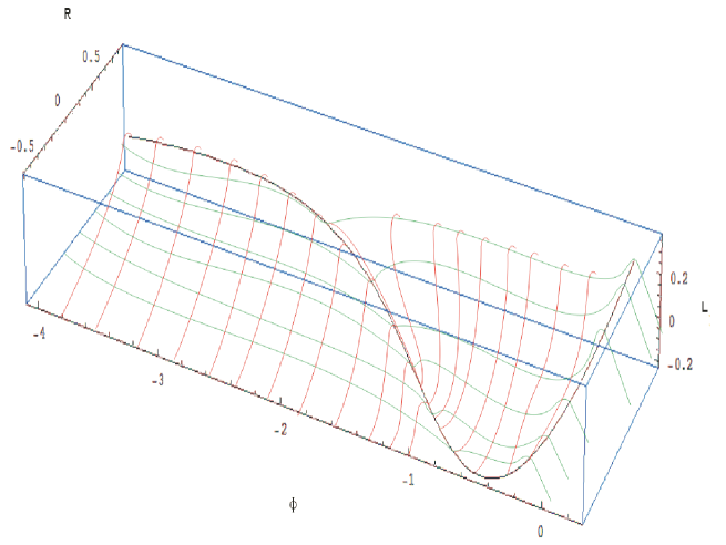
Figure 1: The qualitative form of a Whitney surface with local extrema in the case of a nonlinear curvature Lagrangian $L(R)$ depending on $\phi$ as control parameter.

4.1 Reparametrized Lagrangian

Instead of studying the resulting complicated nonlinear field equations of higher–order curvature Lagrangians, we follow the equivalence proof of Ref. [28] for the conformal frame (22). Then, our inflaton Lagrangian density (2) acquires the form

$${\mathcal{L}}=\frac{1}{2\kappa}\sqrt{\mid g\mid}\left[R\Omega-2\kappa\Omega^{2}{\hat{U}}(\Omega)\right]\,,$$ (24)

where ${\hat{U}}(\Omega):=U(\phi(\Omega))=U\left(\sqrt{3/2\kappa}\ln\Omega\right)$ is the reparametrized potential. Thus in our approach, the inflaton or dark matter scalar will not be regarded as an independent field, but is induced via (23) by the non–Einsteinian pieces of the general Lagrangian $L=L(R)$. Solving for the potential via the method of Helmholz, we obtain

$${\hat{U}}(\Omega)={\mathcal{H}}(R)/\Omega^{2}=\left[\frac{R\Omega}{2\kappa}-L\right]/\Omega^{2}\,.$$ (25)

If we identify the conformal factor with the field momentum via $\Omega=2\kappa d{L}/dR$, the bracket in (25) can be regarded [36] as a Legendre transformation $L\to{\mathcal{H}}(R)=Rd{L}/dR-{L}$ from the original Lagrangian (2) to the general nonlinear curvature scalar Lagrangian $L=L(R)$. Then, the parametric reconstruction

$$R=2\kappa\exp\left(\sqrt{2\kappa/3}\phi\right)\left[2U(\phi)+\sqrt{3/2\kappa}\,\frac{dU}{d\phi}\right]\,,$$ (26)

and

$$L=\exp\left(2\sqrt{2\kappa/3}\phi\right)\left[U(\phi)+\sqrt{3/2\kappa}\,\frac{dU}{d\phi}\right]$$ (27)

of the higher–order effective Lagrangian $L(R)$ from the self–interacting inflaton potential $U(\phi)$ arises [5]. Here the scalar field plays merely the role of a control parameter. The form of the Whitney surface with its local valleys and mountains is qualitatively shown in Fig. 1.

5 Bifurcations with effective ‘dark energy’

In order to model self-interacting dark matter, let us consider the potential

$$U=m^{2}|\phi|^{2}\left(1-\chi|\phi|^{4}\right)\,,$$ (28)

where $m$ is the mass of an ultra-light scalar and $\chi$ the coupling constant of the nonlinear self-interaction. It provides us with a solvable non-topological soliton type model of dark matter halos [44, 45] even with toroidal substructures[46] and a reasonable approximation of the rotation curves of dark matter dominated galaxies. Moreover, the predicted scaling relation [12] fits almost ideally astronomical observations. In Ref. [55] we predicted the effects of such scalar field halos for microlensing.

5.1 Free field

In the string landscape[26], a triple unification of inflation, DM and DE suggests itself based on a simple quadratic potential (28) with $\chi=0$ corresponding to a free massive field. Then, our scalar field toy model likewise incorporates ‘dark energy’ in a rather novel way: The exact parametric solution of the equivalent nonlinear Lagrangian $L(R)$ for the ‘free’ field reads

$$R = 6m^{2}xe^{x}(1+x),$$ (29)

$$L = \frac{3m^{2}}{2\kappa}xe^{2x}(2+x),$$ (30)

where $x:=\ln\Omega$ under the reality condition $\Omega>0$.

Figure 2: The swallow tail behavior of the Lagrangian $L(R)$ for a massive ‘free’ field ($\chi=0$ and $\kappa=m=1$).

The dependence of $L(R)$ given in Fig. 2 is rather surprising and represents the bifurcation set of the swallow tail catastrophe [3, 22, 24] associated with some higher dimensional grand manifolds. The scalar field $\phi$, its mass $m$ as well as $\chi$ play the role of control parameters. According to the theory of singularities (more widely known as catastrophe theory, cf. Arnol’d [3]), this bifurcation set indicates that the Lagrangian manifolds are associated with two local “minima” and one “maximum” (and saddle points at the meeting points of the grand manifold). Each of the “minima” merges with the “maximum” at the cuspoidal points A and B and then disappears. The minima (the semi-infinite segments A and B) are characterized by a positive second derivative of the Hamiltonian ${\mathcal{H}}(\Omega)$ with respect to the momentum $\Omega$, i.e. $d^{2}{\mathcal{H}}/d\Omega^{2}>0$. They correspond to an effective Lagrangian with vanishing cosmological constant.

For the “maximum”, i.e. the segment AB, this derivative is negative and the effective Lagrangian has a modified gravitational constant and a positive cosmological constant,

$$\kappa_{\rm eff}=e\kappa\,,\qquad\Lambda_{\rm eff}=3m^{2}/(2e)\,,$$ (31)

respectively.

Figure 3: Whitney surface for the nonlinear curvature Lagrangian $L(R)$ corresponding to the model (28) with $\chi=0.3$ and $m=\kappa=1$ depending on $\phi$ as control parameter. ($\phi$ in units of $\left[\sqrt{3/(2\kappa)}\right]$.)

5.2 Self-interacting scalar

In the nonlinear case, the exact parametric solution $L(R)$ reads

$$R = 6m^{2}xe^{x}\left[1+x-\frac{27\chi}{4\kappa^{2}}x^{4}-\frac{9\chi}{4\kappa^{2}}x^{5}\right],$$ (32)

$$L = \frac{3m^{2}}{2\kappa}xe^{2x}\left[2+x-\frac{27\chi}{2\kappa^{2}}x^{4}-\frac{9\chi}{4\kappa^{2}}x^{5}\right].$$ (33)

The resulting extremal curve of the Whitney surface is drawn in Fig. 3, and its projections $L=L(R)$, $R=R(\phi)$, and $L=L(\phi)$ in Fig. 4.

Figure 4: Projections of the Whitney surface in Fig. 3 for the nonlinear curvature Lagrangian $L(R)$ corresponding to a nonlinear scalar (28) with $\chi=0.3$ and $m=\kappa=1$.

For $\chi\neq 0$, the bifurcation diagram in Fig. 5 is of higher rank than for the free field. Near the center, we find the butterfly part of the catastrophe. But, for each non-vanishing $\chi$, there exists a further cusp far away from the center, for a large negative $R$ value and $L$ close to zero. From this cusp, the curve finally returns to the origin, for $L$ values very close to zero so that it cannot be seen in Fig. 5 or 6. In an enlargement of the additional cusp in Fig. 7, one can see that $L(R)$ actually becomes negative and forms a cusp.

Figure 5: The wigwam singularity for the nonlinear curvature Lagrangian $L(R)$ for a NTS model with $\chi=0$, 0.1 (long dashes), 0.2 (short dashes), 0.3 (dashed) and $\kappa=m=1$; here only the butterfly part near the center is shown.

The effective strength of gravity and the value of cosmological constant

$$\kappa_{\rm eff}=\kappa e^{-x}\,,\quad\Lambda_{\rm eff}=3m^{2}\frac{x^{2}e^{x}}{x+3}\,,$$ (34)

respectively, depend now on both, the mass $m$ and, via $x$ as a solution of $R=0$, on the coupling constant $\chi$ of the scalar field, and need to be constrained by cosmological data.

Figure 6: For the NTS model with $\chi=0.3$ and $\kappa=m=1$, the wigwam catastrophe of the Lagrangian $L(R)$ can be decomposed into a butterfly plus additional elementary catastrophe. Here, the butterfly catastrophe arises near the origin; at about $(R,L)=(-250,-0.015)$ there is a further cusp, cf. Fig. 7; the curve finally returns to the origin which cannot be seen due to our scale.

In quintessence models [66], e.g., the crossover scale of the scalar field is $|\phi_{\rm c}|=\exp(-1/\alpha)M_{\rm Pl}^{2}/m$, where $\alpha=1/138$ is about Sommerfeld’s fine structure constant and $M_{\rm Pl}=1/\sqrt{\kappa}$ the reduced Planck mass. Then the tiny observed cosmological constant of the present epoch

$$\Lambda_{\rm DE}=m^{2}\phi_{\rm c}^{2}=\exp(-2/\alpha)M_{\rm Pl}^{4}\simeq(10^{-3}{\rm eV})^{4}$$ (35)

is roughly reproduced for small $\chi$.

Figure 7: Continuation of Fig. 6. Enlarging the additional cusp for the nontopological soliton field with $\chi=0.3$ and $\kappa=m=1$.

It is important to stress that within the range limited by cuspoidal points, all three states may coexist with each other. Thus our bifurcation set, cf. Ref. [56] for a generalization with $\chi\neq 0$, indicates that each local patch of the Universe may have a different strength and cosmological constant (‘dark energy’) controlled by the mass $m$ of the scalar field, but the effective Lagrangian has approximately the same Einsteinian form (1). In “maximal” domains, inflation may be still going on, thus realizing prospective ideas of Linde [27].

5.3 Natural inflation from the axion?

In QCD, after integrating out the fermion fields, its generating functional including a topological Pontrjagin term for the Yang-Mills gauge fields induces an effective axion potential

$$U=\Lambda_{\rm QCD}^{4}\left[1-\cos(\phi/f_{\phi})\right].$$ (36)

This potential displays a periodicity with a period of $2\pi f_{\phi}$, has a minimum at $\phi=0$, as required, and leads to the induced axion mass of $m_{\phi}=\Lambda_{\rm QCD}^{2}/f_{\phi}$. A quintaxion may also be induced by spacetime torsion[40].

Within natural inflation[52], such a potential has been proposed for an axion coupling constant close to the Planck scale. For simplicity let us assume in the following that $f_{\phi}\simeq\sqrt{3/(2\kappa)}$. Then, following the general prescription (26)-(27), we find the reparametrized solution

$$R = 2\kappa\exp\left(x\right)\Lambda_{\rm QCD}^{4}\left[2-2\cos\left(x\right)+\sin\left(x\right)\right]\;,$$ (37)

$$L = \exp\left(2x\right)\Lambda_{\rm QCD}^{4}\left[1-\cos\left(x\right)+\sin\left(x\right)\right]\;.$$ (38)

Fig. 8 exhibits a swallow tail behavior similar as for a NTS potential with $\chi=0$.

Figure 8: The axion gives rise again to a swallow tail catastrophe in the Lagrangian $L(R)$, with the choice of $\Lambda_{\rm QCD}=0.1$, $\kappa=1$, and $f_{\phi}=1$.

6 Domain structure of dark matter and induced dark energy

Baryonic particles (such as protons and neutrons) account for visible matter in the Universe, that is only a small fraction of the observed total matter. The major part of it is a mysterious DM, which only interacts gravitationally. On the other hand according to our model, the Universe splits into almost Einsteinian domains with – depending on the physical scale and eras – a different gravitational strength and cosmological constant, the latter being most likely a representation of DE. A natural question is how these domains arise? To answer this, we have to look into the initial inflationary stage of the Universe, long before decoupling of radiation and matter, even before grand unified phase transitions where only an initial pre-field existed. At the initial stage of the quantum era, the fundamental pre-field may have existed in a form of a scalar or vector gauge fields. Without lack of generality we can limit ourselves to a scalar field $\phi$.

During this quantum era, the scalar field was strongly fluctuating. Due to the rapid inflation, the size of the Universe as well as the size of each individual fluctuation have increased enormously while the amplitude remains almost the same. During this fast spacelike expansion, just after the stretching, these space fluctuations of $\phi$ were frozen while loosing their quantum nature due to the increasing size. The decoupling of radiation and visible matter has imprinted fluctuations on the electromagnetic spectrum which we observe now in the anisotropy microwave background radiation. However, we cannot see such ripples of the visible matter after the decoupling. Due to the gravitational interaction the process of large scale formation has started just after the decoupling. And the state of nearly homogeneously distributed visible matter existing after the decoupling has eventually been transformed into clusters of galaxies and star structures which we see nowadays. Obviously, the decoupling of the dark part of matter from radiation and visible matter may have happen even earlier, when the Universe was in the form of a quark-gluon plasma. However, after decoupling the dark part of matter must be subjected to the same gravitational forces and to a similar large scale formation. Since its total mass is significantly larger than the visible mass, the formation of large structures of DM may have a weak influence on the visible matter.

Dark matter will have an opposite effect by dictating where and how the visible matter should be distributed, probably localized around clusters of DM. In the case of scalar field DM, its peculiarities such as self-interaction may also have contributed to the DE distribution. DM cannot be seen directly by traditional observations but can be inferred from more sophisticated gravitational lensing[29], revealing that DM exists in a form of a loose network of filaments, growing over time, which intersect in massive structures at the locations of clusters of galaxies. This finding is consistent with the conventional theory of large scale structure formation, where a smooth distribution of DM collapses first into filaments and then into clusters, forming a cosmic scaffold[29], then accumulating visible matter and later newly born stars.

The primary candidate for DM is a scalar field. If a scalar field exists, then it may have different amplitudes or different mass densities in different space regions. Such a distribution of $\phi$ has been created after the inflation of the Universe. It is associated with different amplitudes of the frozen fluctuations. The process of large scale structure formation is rather similar in each of these regions. Our results indicate that in each of these different regions the gravitational constant may vary[56], depending on the amplitude of the scalar field of the given frozen space fluctuation. In other words, in each of these regions defined by the original frozen fluctuations there will arise different Newtonian potentials. This is consistent with recent studies[10] showing that, during expansion, a vector field having two different initial amplitudes will give rise to different Newtonian potentials. This difference in turn drives self-consistently enhanced growth of the density perturbations which enables tiny perturbations to grow into the large structures we see today.

6.1 Cosmic domains

Our studies indicate that these different Newtonian potentials correspond to different effective gravitational constants in various regions of the Universe. If this is true, the data of recent observations[29] should be reinvestigated. In regions with larger gravitational constants one may see that the gravitational lensing will be stronger and vice versa. We regard areas with different gravitational potentials as cosmic domains characterized by their own gravitational and cosmological constants. There occurs a coexistence of these domains (which primordially may be of topological origin[19, 20]). On the boundaries of the domains, changes in the gravitational and cosmological constants are expected to be abrupt. In spite of the random or fluctuational origin of these domains, the values of these gravitational and cosmological constants take only a few universal numbers, corresponding to only a finite number of types of domains.

For small curvature, each of these states can be described approximately by the same effective Lagrangian (1) with different gravitational constant $\kappa_{\rm eff}$ and cosmological constant $\Lambda_{\rm eff}$ and emerge as a fixed point of the conformal transformation from one side and universal classes of the smooth differential mappings from the other side[22]. These spaces are approximately Einstein spaces, but of different gravitational strength as well as with different cosmological constants. The distribution of such cosmological constants in the Universe corresponds to DE induced by the scalar field distribution. On a very large scale, $\phi$ is homogeneously distributed and therefore we expect that DE will be distributed homogeneously, depending on the details of inflationary cosmology.

6.2 Domains arising from free fields

If DM and DE were associated with a massive free scalar field gravitationally coupled or/and associated with axions (see, Sec. 5.3) there will arise three types of domains:

1) The first type of domains, I, is described by Einstein‘s theory with conventional gravitational constant and vanishing cosmological constant.

2) The second type of domains, II, is described by an Einsteinian model having a very large gravitational constant and a vanishing cosmological constant. Such type of domains may be gravitationally unstable, leading eventually to their contraction and ultimately to a gravitational collapse and phenomena resembling supernova explosions. For very large masses, we may expect that these explosion will be stronger than standard supernovae. Our approach may explain the fact why some supernovae progenitors seem to have exceeded[16] the Chandrasekhar limit.

3) The third type of domains, III, are described by an Einsteinian model with large gravitational and positive cosmological constant $\Lambda^{\rm III}_{\rm eff}$ given by (34). Then we expect that such domains are still expanding according to effective Friedman equations and probably their sizes are also increasing. Such expansion may be ended abruptly and such domains will be transformed into domains of type I.

One may speculate that the largest part of the Universe is occupied by domains of type I, corresponding to spaces with zero cosmological constant. The next largest proportion of the Universe is expected to be occupied by domains of type III. Those parts of the Universe occupied by domains of type II are decreasing with time. Each disappearance of such domain would be accompanied by supernova type explosions.

On the average, the cosmological constant inferred from recent observations is

$$\Lambda_{\rm DE}=\frac{V_{\rm III}\Lambda^{\rm III}_{\rm eff}}{V_{\rm I}+V_{\rm II}+V_{\rm III}},$$ (39)

where the spacelike volumes $V_{\rm I},V_{\rm II}$ and $V_{\rm III}$ are associated with domains of type I, II, and III, respectively.

In summary, our bifurcation set (see Fig. 1 and Fig. 2) indicates that the Universe is locally described by Einstein’s GR and effectively split into domains. The splitting originated from primordial quantum fluctuations which were frozen during inflation. Each domain or local patch of the Universe may have different gravitational strength and may have zero or negative pressure associated with DE. In domains of type II associated with a positive cosmological constant the inflation may be still going on. It will be stopped exactly at the bifurcation point A and this domain will be transformed into a domain of type I, as in Fig. 2. For a massive free scalar field and for axions the bifurcation set is the swallow tail catastrophe. There are two cusps at the points A and B which are associated with the highest singularities of the differential mappings. They are also related to the domain boundaries. In each of these cuspoidal points A and B of the bifurcation diagram, the minimum of some grand manifold merges with the maximum[23]. Each local minimum (the segment A and the semi-infinite segment B) is associated with two types of domains, I and II, respectively. Each local maximum (saddle) of the grand manifold is associated with an expanding domain of type III (the segment AB). The effective Einsteinian gravity for this domain is stronger than that in the domain of type I, depending on the mass of the scalar field. Domains with a positive effective cosmological constant are still in an expanding inflationary phase.

The ‘strong’ gravity state, the domain II (the semi-infinite segment B) with a negative or vanishing cosmological constant corresponds to deflation. Since the Universe is split into dynamical regions associated with different gravity, their boundaries change with time and present some kind of cosmological strings or membranes. Changes of the boundary are associated with some sort of local phase transition reminding us of phase separations like those arising in first order phase transitions. At some instant, all these domains are in quasi-equilibrium with each other although their boundaries changes with time as the membranes are moving. At very long time scales (much larger than the Planck time) when inflation in the domains of type III will eventually be ceased, only stable phases, like the domains of type I and some small concentration of domains of type II will remain. These domains would produce explosions resembling supernovae with masses well beyond of the Chandrasekhar limit, similar to those observed[16].

6.3 Domains arising from self-interacting fields

In case of self-interacting scalar fields with $\chi\neq 0$, the classification will be richer (see Figures 4, 5 and 6), with five types of domains. The bifurcation diagram associated with such a wigwam catastrophe or $A_{5}$ singularity according to Arnold’s classification[3] consists of four cusps or four $A_{2}$ singularities, with a dramatic change in the gravitational and cosmological constants.

There occurs a general decoupling of the wigwam catastrophe $A_{5}$ into a butterfly catastrophe $A_{4}$, and the elementary cusp $A_{2}$, depending on the values of $R$: If the butterfly catastrophe arises near the origin or at small values of $R$, the additional cuspoidal point is associated with a very large value of $R\simeq-250$. For some fixed values of the coupling constant $\chi=0.1$, 0.2, 0.3, the butterfly part of bifurcation diagram is presented in Figs. 5. In comparison with the free massive field, the inclusion of the self-interaction associated with the nonzero parameter $\chi$ gives rise to two extra cusps leading to the appearance of two extra branches in the bifurcation diagram, again associated with effective Einsteinian spaces. Although these almost linear branches do exist at positive $R$, their major part is related to negative values of $R$. For one of these branches the cosmological constant vanishes while for the other one the cosmological constant decreases when the value of $\chi$ increases, and the part of the branch associated with $R>0$ decreases. In general, the self-interaction induced by the field $\phi$ increases the strength of gravity and decreases the cosmological constant.

Let us describe in more detail the transitions in the bifurcations: Starting from the first branch, denoted as I, through the first cuspoidal point we arrive at the second branch II which is very similar to the case of a free massive scalar field, although its length decreases significantly when $\chi$ increases and the cosmological constant vanishes at any value of $\chi$. This branch corresponds to the limit $\phi\rightarrow 0$ of small scalar fields, corresponding to the conformal factor $\Omega=1$. Therefore, on this branch we recover the linear Hilbert-Einstein Lagrangian $L_{\rm HE}=R/2\kappa$, as expected. With decreasing $\Omega$, we will come to the next cuspoidal point, where the new branch III has a positive cosmological constant and gravity becomes stronger. With increasing value of $\chi$ the length of this branch increases. Thus, there will be more domains having positive cosmological constant and a gravitational strength higher than the conventional. By decreasing $\Omega$ until reaching the next cuspoidal point of the bifurcation diagram, we arrive at the branch IV. The spacetime associated with this branch has a very strong gravity and negative cosmological constant. Similar to the free massive case, this branch probably is gravitationally unstable. Finally, for very small $\Omega$, we will arrive at the branch V with $R<0$, where gravity is the strongest but without cosmological constant. Similar to the previous branch IV, the domain V is unstable, as well. Thus in a Universe filled with self-interacting scalar fields, we would expect that a rather strong phase separation into further domains will arise.

7 Discussion

For dilute DM the Lagrangian has the standard Hilbert-Einstein form $L_{\rm HE}=R/2\kappa$. For dense DM, i.e. large values of the DM scalar, the resulting effective Lagrangian is $L_{\rm HE}=R/2\kappa_{\rm eff}$, only the slope is less steep, i.e. the effective gravitational coupling $\kappa_{\rm eff}>\kappa$ is, by “renormalization” [66, 4], larger than Newton’s. This resembles some aspects of MOND, but with the advantage that we still work in the standard general relativistic framework. Depending on its sign, the cosmological constant $\Lambda_{\rm eff}$ in a bifurcation approximated for small $R$ by (1) can also model DE or an accelerating phase of the present epoch of the Universe (like ‘anti-gravity’). There also may arise “gravitational screening” for $\kappa_{\rm eff}$ smaller than Newton’s. MACHOs can now be described by some specific nonlinear modifications of the Hilbert-Einstein action.

In the light of our finding we have to comment on recent observations[30], which constrain the density of MACHO type objects in the Universe by measuring the brightness of high redshift type Ia supernovae relative to low redshift samples. These data favor DM made of microscopic particles (such as WIMPs) or scalar and vector gauge fields over MACHOs with masses between $10^{-2}$ and $10^{10}$ solar masses. This provides another evidence that our approach correctly describes the frozen space fluctuations which lead to a formation of cosmic domains with a different density of DM and DE in the Universe.

References

- [1]
- [2] S. Ando, “Can dark matter annihilation dominate the extragalactic gamma-ray background?”, Phys. Rev. Lett. 94, 171303 (2005).
- [3] V.I. Arnol’d: Catastrophe Theory, Third, revised and expanded edition (Springer-Verlag, Berlin 1992).
- [4] J.D. Bekenstein, “Relativistic gravitation theory for the MOND paradigm”, Phys. Rev. D 70, 083509 (2004).
- [5] J. Benítez, A. Macías, E.W. Mielke, O. Obregón, and V.M. Villanueva, “From inflationary COBE potentials to higher–order curvature scalar Lagrangians”, Int. J. Mod. Phys. A 12, 2835 (1997).
- [6] L. Bergström, J. Edsjö, M. Gustafsson, and P. Salati, “Is the dark matter interpretation of the EGRET gamma excess compatible with antiproton measurements?”, JCAP 0605, 6 (2006).
- [7] S.M. Carroll, V. Duvvuri, M. Trodden, and M.S. Turner, “Is cosmic speed-up due to new gravitational physics?”, Phys. Rev. D 70, 043528 (2004).
- [8] S.M. Carroll, I. Sawicki, A. Silvestri, and M. Trodden, “Modified-source gravity and cosmological structure formation”, New Journal of Phys. 8, 323 (2006).
- [9] W. de Boer, “Evidence for dark matter annihilation from galactic gamma rays?”, New Astron. Rev. 49, 213 (2005).
- [10] S. Dodelson and M. Liguori, “Can cosmic structure form without dark matter?”, Phys. Rev. Lett. 97, 231301 (2006).
- [11] B. Fuchs, “Constraints on the decomposition of the rotation curves of spiral galaxies”, Proc. of the 4th International Workshop on the Identification of Dark Matter (IDM 2002), York, England, 2-6 Sep 2002, e-Print: astro-ph/0212485.
- [12] B. Fuchs and E.W. Mielke, “Scaling behaviour of a scalar field model of dark matter haloes”, Mon. Not. R. Astron. Soc. 350, 707–709 (2004).
- [13] M.K. Gaillard and B. Kain, “Is the universal string axion the QCD axion?”, Nucl. Phys. B 734, 116 (2006).
- [14] A. García, A. Macías, and E.W. Mielke, “Stewart–Lyth second–order approach as an Abel equation for reconstructing inflationary dynamics”, Phys. Lett. A 229, 32 (1997).
- [15] H. Hoekstra, H.K.C. Yee, and M.D. Gladders, “Properties of galaxy dark matter halos from weak lensing”, Astrophys. J. 606, 67 (2004).
- [16] D.A. Howell et al., “The type Ia supernova SNLS-03D3bb from a super-Chandrasekhar-mass white dwarf star”, Nature 443, 308-311 (2006).
- [17] W. Hu, R. Barkana, and A. Gruzinov, “Fuzzy cold dark matter: The wave properties of ultralight particles”, Phys. Rev. Lett. 85, 1158 (2000).
- [18] K.R.W. Jones and D. Bernstein, “The self-gravitating Bose-Einstein condensate”, Class. Quantum Grav. 18, 1513 (2001).
- [19] T.W.B. Kibble, “Some implications of a cosmological phase transition”, Phys. Rept. 67, 183 (1980).
- [20] T.W.B. Kibble, “Symmetry breaking and defects”, arXiv:cond-mat/0211110.
- [21] W.H. Kinney, E.W. Kolb, A. Melchiorri, and A. Riotto, “Inflation model constraints from the Wilkinson microwave anisotropy probe three-year data”, Phys. Rev. D 74, 023502 (2006).
- [22] F.V. Kusmartsev, “Application of catastrophe theory to molecules and solitons”, Phys. Rept. 183, 1 (1989).
- [23] F.V. Kusmartsev, E.W. Mielke, Yu.N. Obukhov, and F.E. Schunck, “Classification of inflationary Einstein–scalar–field–models via catastrophe theory”, Phys. Rev. D 51, 924 (1995).
- [24] F.V. Kusmartsev, E.W. Mielke, and F.E. Schunck, “Gravitational stability of boson stars”, Phys. Rev. D 43, 3895 (1991).
- [25] F.V. Kusmartsev, E.W. Mielke, and F.E. Schunck, “Stability of neutron and boson stars: a new approach based on catastrophe theory”, Phys. Lett. A 157, 465 (1991).
- [26] A.R. Liddle and L.A. Urena-Lopez, “Inflation, dark matter and dark energy in the string landscape”, Phys. Rev. Lett. 97, 161301 (2006).
- [27] A. Linde: Inflation and Quantum Cosmology (Academic Press, San Diego, 1990).
- [28] G. Magnano and L.M. Sokolowski, “Physical equivalence between nonlinear gravity theories and a general–relativistic self–gravitating scalar field”, Phys. Rev. D 50, 5039 (1994).
- [29] R. Massey et al., “Dark matter maps reveal cosmic scaffolding”, Nature 445, 286-290 (2007).
- [30] R.B. Metcalf and J. Silk, “New constraints on macroscopic compact objects as dark matter candidates from grav. lensing of type Ia supernovae”, Phys.Rev.Lett. 98, 071302 (2007).
- [31] E.W. Mielke, “Conformal changes of metrics and the initial–value problem of general relativity”, Gen. Rel. Grav. 8, 321 (1977).
- [32] E.W. Mielke, “Note on localized solutions of a nonlinear Klein–Gordon equation related to Riemannian geometry”, Phys. Rev. D 18, 4525–4528 (1978).
- [33] E.W. Mielke, “Mass formular for solitons with quantized charge”, Lett. Nuovo Cim. 25, 424 (1979).
- [34] E.W. Mielke, “On pseudoparticle solutions in Yang’s theory of gravity”, Gen. Rel. Grav. 13, 175–187 (1981).
- [35] E.W. Mielke, B. Fuchs, and F.E. Schunck: “Dark matter halos as Bose-Einstein condensates”, Proc. of the Tenth Marcel Grossman Meeting on General Relativity, Rio de Janeiro, 2003, M. Novello, S. Perez-Bergliaffa, and R. Ruffini, eds. (World Scient., Sing. 2006), p. 39–58.
- [36] E.W. Mielke and F.W. Hehl, “Comment on: General relativity without the metric”, Phys. Rev. Lett. 67, 1370 (1991).
- [37] E.W. Mielke and H.H. Peralta, “Eigenvalues of the third order slow-roll approximation of inflation”, Phys. Rev. D 66, 123505 (2002).
- [38] E.W. Mielke and H.H. Peralta, “Flattened halos in a nontopological soliton model of dark matter”, Phys. Rev. D 70, 123509 (2004).
- [39] E.W. Mielke and A.A. Rincón Maggiolo, “Duality in Yang’s theory of gravity”, Gen. Rel. Grav. 37, 997–1007 (2005).
- [40] E.W. Mielke and E.S. Romero (2006), “Cosmological evolution of a torsion-induced quintaxion”, Phys. Rev. D 73, 043521 (2006).
- [41] E.W. Mielke and F.E. Schunck, “Reconstructing the inflaton potential for an almost flat COBE spectrum”, Phys. Rev. D 52, 672 (1995).
- [42] E.W. Mielke and F.E. Schunck, “Boson stars: Alternatives to primordial black holes?”, Nucl. Phys. B 564, 185 (2000).
- [43] E.W. Mielke and F.E. Schunck, “Are axidilaton stars massive compact halo objects?”, Gen. Rel. Grav. 33, 805–813 (2001).
- [44] E.W. Mielke and F.E. Schunck, “Non-topological scalar soliton as dark matter halo”, Phys. Rev. D 66, 023503 (2002).
- [45] E.W. Mielke, F.E. Schunck, and H.H. Peralta, “Scalar soliton in Newtonian gravity modelling dark matter halos”, Gen. Rel. Grav. 34, 1919–1930 (2002).
- [46] E.W. Mielke and J.A. Vélez Pérez, “Toroidal halos in a nontopological soliton model of dark matter”, Phys. Rev. D 75, 043504 (2007).
- [47] J. Milnor: Lectures on Morse Theory, Ann. Math. Studies No. 51 (Princeton University Press, Princeton, New York, 1963).
- [48] F. Mueller-Hoissen, “From Chern-Simons to Gauss-Bonnet”, Nucl. Phys. B 346, 235 (1990).
- [49] S. Nojiri and S.D. Odintsov, “Modified f(R) gravity consistent with realistic cosmology: From matter dominated epoch to dark energy universe”, Phys. Rev. D 74, 086005 (2006).
- [50] O. Obregon, L.A. Urena-Lopez, and F.E. Schunck, “Oscillatons formed by nonlinear gravity,” Phys. Rev. D 72, 024004 (2005).
- [51] R.D. Peccei, “Reflections on the strong CP problem”, Nucl. Phys. Proc. Suppl. 72, 3 (1999).
- [52] C. Savage, K. Freese, and W.H. Kinney, “Natural inflation: Status after WMAP 3-year data”, Phys. Rev. D 74, 123511 (2006).
- [53] R. Schimming and H.J. Schmidt, “On the history of fourth order metric theories of gravitation”, NTM Schriftenr. Gesch. Naturw. Tech. Med. 27, 41 (1990).
- [54] F.E. Schunck, “A scalar field matter model for dark halos of galaxies and gravitational redshift”, astro-ph/9802258.
- [55] F.E. Schunck, B. Fuchs, and E.W. Mielke, “Scalar field haloes as gravitational lenses”, Mon. Not. R. Astron. Soc. 369, 485–491 (2006).
- [56] F.E. Schunck, F.V. Kusmartsev, and E.W. Mielke, “Dark matter problem and effective curvature Lagrangians”, Gen. Rel. Grav. 37, 1427–1433 (2005).
- [57] F.E. Schunck and E.W. Mielke, “A new method of generating exact inflationary solutions”, Phys. Rev. D 50, 4794 (1994).
- [58] F.E. Schunck and E.W. Mielke, “Eigenvalues of the Stewart–Lyth equation for inflation with a blue spectrum”, Phys. Lett. B 485, 231–238 (2000).
- [59] F.E. Schunck and E.W. Mielke, “TOPICAL REVIEW: General relativistic boson stars”, Class. Quantum Grav. 20, R301 (2003).
- [60] F.E. Schunck and O. Obregón, “Self-gravitating complex scalar fields conformally transformed into higher-order gravity: Inflation and boson stars”, preprint (1997).
- [61] D.N. Spergel and P.J. Steinhardt, “Observational evidence for self-interacting cold dark matter”, Phys. Rev. Lett. 84, 3760 (2000).
- [62] D.N. Spergel et al., “First-year Wilkinson microwave anisotropy probe (WMAP) Observations: Determination of cosmological parameters”, Astrophys. J. Suppl. 148, 175 (2003); “Wilkinson microwave anisotropy probe (WMAP) three year results: Implications for cosmology”, arXiv:astro-ph/0603449.
- [63] A.A. Starobinsky, “A new type of isotropic cosmological models without singularity”, Phys. Lett. 91B, 99 (1980).
- [64] R.C. Tolman: Relativity, Thermodynamics, and Cosmology (Clarendon Press, Oxford 1934).
- [65] D. Vassiliev, “Pseudoinstantons in metric affine field theory”, Gen.Rel.Grav. 34, 1239 (2002).
- [66] C. Wetterich, “Conformal fixed point, cosmological constant, and quintessence”, Phys. Rev. Lett. 90, 231302 (2003).
- [67] K. Zioutas, D.H.H. Hoffman, K. Dennerl, and Th. Papaevangelou, “What is dark matter made of?”, Science 306, 1485 (2004).