We have extensively mapped a sample of dense molecular clouds (L1512, TMC-1C, L1262, Per 7, L1389, L1251E) in lines of HC₃N, CH₃OH, SO and C¹⁸O. We demonstrate that a high degree of chemical differentiation is present in all of the observed clouds. We analyse the molecular maps for each cloud, demonstrating a systematic chemical differentiation across the sample, which we relate to the evolutionary state of the cloud. We relate our observations to the cloud physical, kinematical and evolutionary properties, and also compare them to the predictions of simple chemical models. The implications of this work for understanding the origin of the clumpy structures and chemical differentiation observed in dense clouds are discussed.  

1 Introduction

Low-mass stars form in dense cloud cores. Understanding how stars form thus requires detailed knowledge of the physical and chemical evolution of molecular clouds. The classic picture, in which star formation is magnetically-dominated and mediated by ambipolar diffusion [e.g. 1], posits long molecular cloud lifetimes ($\sim 10^{7}$ years). However, there is an increasing realisation that dissipation of turbulence, driven externally at large scales, plays a vital role [e.g. 2]. In this case, star formation is dynamic and rapid, and molecular cloud lifetimes are short ($\sim 10^{5}-10^{6}$ years). Dense cloud chemistry will follow different evolutionary paths depending upon the lifetime of molecular clouds, and hence on the time-scale of low-mass star formation [e.g. 3]. One may also expect that the spatial distribution of molecules should also reflect the underlying cloud dynamics. Observations of dense interstellar clouds in a variety of molecular tracers show that they contain a distribution of dense gaseous structures [4]. These structures exhibit a size distribution ranging from that of dense cores [$\sim 0.05-0.1$ pc, 5], to clumps [$\sim 0.01-0.05$ pc, 6, 7] down to so-called small clumpinos [$\sim 0.005$ pc, 8]. The spatial distributions of molecules in cold, apparently quiescent, clouds do appear to show chemical abundance gradients, i.e. chemical differentiation. Previously, the best studied sources have been the clouds TMC-1 and L134N [9, 10, 11]. These clouds show striking differences in the location of the emission peaks in several molecules. In TMC-1, for example, emission from the carbon chain molecules (e.g. the cyanopolyynes) is observed to be anticorrelated with that of ammonia and $\rm N_{2}H^{+}$ and several deuterated species [e.g. 12, 13, 14]. These clouds also show distinct emission peaks from other specific molecules, such as methanol and SO. High resolution observations show that chemical differentiation is present at all spatial scales [8, 15, 16]. Although, in dense cores, depletion of CO, CS and other heavy molecules on to dust grains is undoubtedly important [17, 18], the reason for the spatial differentiation seen amongst other molecules is unclear, as is its prevalence in other molecular clouds.

It is possible that there is a link between the observed chemical differentiation and the clumpy structure, and hence to the physical origin of clumps through the cloud turbulence. There are currently two possibilities [see 19, 20]. First, numerical simulations show that dissipation of externally driven turbulence can produce structures, similar to the clumps and cores that are observed, through the process of ‘turbulent fragmentation’ [2]. Second, winds and outflows have a significant effect on the structure and evolution of the surrounding protostellar envelope, containing energies sufficient to physically disrupt the envelope material and to alter the chemistry. These outflows begin very early in the star formation process, and cloud turbulence could be excited by them [21]. In this case, the cloud structure is regulated by the action of stars [e.g. 22]. The presence of parsec-scale flows [e.g. 23] and wind blown bubbles [24] are clear observational evidence that protostars affect their environment in this way, and that the influence of existing star formation can have a very long reach. In this picture, the turbulence should be a function of the local star-formation activity, however it is unclear if enough kinetic energy can be injected in all clouds to sustain the observed level of turbulence. As the nature of the turbulence should affect the formation and evolution of clumpy structure, we might therefore expect that there should be chemical differences between starless cores and those containing protostars at the Class 0 and/or Class I stages [25], with the former being the product solely of turbulent fragmentation. Models have previously been developed of the spatial and temporal chemical evolution in clumpy molecular clouds [e.g. 17, 26, 27, 28, 29, 30, 31], but with limited success.

To quantify the chemical effects that embedded protostars may have on cloud structure and chemistry, we have previously mapped the Barnard 5 cloud (B5) in many molecular lines. B5 is an active region of star formation in Perseus and contains molecular outflows, wind-blown bubbles, and regions where the outflows appear to be interacting with dense clumps [32, 33, 34]. Most previous observations have focused on the region containing the Class I source, B5 IRS1, and the molecular distributions over the rest of the cloud were previously poorly known. These observations revealed a high degree of spatial differentiation, with similarities to the molecular distributions in TMC-1 [35], but also to some other starless cores in Taurus [36]. Comparison with dynamical-chemical models of B5 [26], based on the Norman & Silk [22] picture, appear to indicate that molecular ices are continually being formed and destroyed [7, 36], but that processes not included in these models must be responsible. However, B5 is only one such source; to constrain any chemical models multi-molecule maps of more sources are needed, for example, to see if similar molecular differentiation occurs in dense clouds with varying degrees of star formation activity and protostellar evolution. We have therefore increased our sample to observe dense core chemistry in different natal environments: starless cores, and those containing young stellar objects (YSOs) at the Class 0 and Class I phases. The sources were selected from the sample mapped by Caselli et al. [37] in N₂H⁺ at 0.063 km s^-1, 54^′′ resolution; lower resolution ammonia maps also exist [5]. Caselli et al. [37] found that the position of the N₂H⁺ peak emission tended to be close to the position of peak $\rm NH_{3}$ emission but generally not coincident with that of the star. From our B5 observations, we found that several molecules are strongly anticorrelated with $\rm N_{2}H^{+}$ and $\rm NH_{3}$ emission at small scales, as well as with each other (e.g. methanol and the carbon chains). Hence, the N₂H⁺ maps of Caselli et al. [37] can be useful to predict where other molecules could be expected to peak in a cloud, assuming the chemical differentiation has the same underlying cause.

The six cores we observed have a range of star-forming activity (see Table 1). TMC-1C is a starless core, with a region of diffuse sub-mm emission to the south, which extends in a ridge beyond our map to the north [38]. This cloud has previously been mapped in carbon chain molecules [39] and in methanol and HC¹³O⁺ [8]. L1389 is associated with an IRAS source, IRAS 04005+5647, although it has been classified as pre-stellar, or an extremely young protostellar source [40]. L1262 contains both a stellar core, IRAS 23238+7401, which drives a protostellar outflow, and a starless core [41]. L1251E contains a YSO, IRAS 22385+7457, which drives an outflow, as well as two infrared sources likely to be T Tauri stars [42]. There are also several infrared sources in the immediate vicinity of our map. L1512 is a starless core, containing a north-south ridge of diffuse sub-mm emission [41]. Per7 contains a sub-mm peak in addition to the Class I source, IRAS 03295+3050 [23].

Table 1: Core Properties

Core	RA(1950)	DEC(1950)	Class	$V_{\rm lsr}$	D
				(km s-1)	(pc)
Per7	03:29:39.5	+30:49:50	I	6.81	350
L1389	04:00:38.0	+56:47:59	prestellar/0	-4.65	600
TMC-1C	04:38:34.5	+25:55:00	prestellar	5.27	140
L1512	05:00:54.4	+32:39:00	prestellar	7.11	140
L1251E	22:38:36.4	+74:55:50	mixed	-3.93	350
L1262	23:23:32.2	+74:01:45	0	4.11	200

We chose to observe four molecular species (see Table 2). The isotope $\rm C^{18}O$ serves to trace much of the low density ($\sim 10^{3}~{}\rm cm^{-3}$) material in the cloud. Methanol is formed solely on grains in dense clouds [e.g. 43]. Once desorbed into the gas, methanol molecules only have a finite lifetime until they are destroyed. Hence, the CH₃OH distribution provides an excellent observational measure of the degree of gas-grain cycling in clumpy clouds. Cores showing weak methanol emission will tend to be older since any CH₃OH liberated previously will gradually re-accrete back onto the dust. As we discovered a new ’cyanopolyyne-peak’ position in B5, similar to that in TMC-1 [35], we also mapped the cyanoacetylene emission in these clouds. The formation and destruction of cyanopolyynes can provide information on those molecules returned to the gas, and also define chemical time-scales in dynamically-evolving clouds [29]. Markwick et al. [29] concluded that such chemically interesting positions should appear to be offset from the position of any YSO present; as well as from the peak ammonia emission. The detection of these organic molecule ‘hotspots’ is thus only possible by making large-scale ${\rm HC_{3}N}$ maps, to include positions distinct from the nominal (0,0) positions of previous searches [cf. 27]. The HC₃N transition chosen traces gas at densities above $\sim 10^{5}~{}\rm cm^{-3}$. Finally, to explain the large number of S-bearing molecules detected in dense clouds, chemical models infer that elemental sulphur is only modestly depleted in dense clouds, relative to more refractory elements [45]. Interstellar sulphur chemistry involves primarily neutral reactions, and so it defines yet another, albeit slow, chemical time-scale. Shock chemistry or grain-surface catalysis have been proposed to be important for S chemistry [30, 46]; the latter mechanism is supported by the detection of OCS in interstellar ices [47]. We therefore mapped the $J_{\rm K}=3_{2}-2_{1}$ line of SO.

Table 2: Molecular Line Properties

Molecule	Transition	Frequency	Eupper	Einstein A	ncrit
		(GHz)	(K)	(s-1)	(cm-3)
C18O	1$\rightarrow$0	109.782	5.27	6.30 $\times 10^{-08}$	$2\times 10^{3}$
SO	2${}_{3}\rightarrow$12	99.300	9.22	1.10 $\times 10^{-05}$	$3\times 10^{5}$
HC3N	10$\rightarrow$9	90.979	24.01	5.81 $\times 10^{-05}$	$7\times 10^{5}$
CH3OH	2${}_{1}\rightarrow$11(E)	96.739	12.55	2.56 $\times 10^{-06}$	$1\times 10^{5}$
	2${}_{0}\rightarrow$10(A+)	96.741	6.97	3.38 $\times 10^{-06}$	$5\times 10^{4}$
	2${}_{0}\rightarrow$10(E)	96.744	20.11	3.41 $\times 10^{-06}$	$4\times 10^{4}$
	2${}_{1}\rightarrow$11(E)	96.755	28.04	2.62 $\times 10^{-06}$	$5\times 10^{4}$

The plan of the paper is as follows. In Section 2 we describe the observations and how the data analysis was performed. In Section 3, we detail the chemical morphology of each source and note the general trends we see in chemical differentiation. Simple chemical models of the chemical evolution in clumpy media are presented and compared to the observational data in Section 4. Conclusions from this study are given in Section 5.

2 Observations, Data Reduction and Analysis

Single dish maps of HC₃N, SO, CH₃OH and C¹⁸O transitions at 3mm were made using the Onsala 20m telescope, Sweden, in April 2005. With the exception of CH₃OH, the spectra were observed in frequency-switched mode, using 12.5 kHz channels to provide a velocity resolution of $\sim$0.04 km s^-1. CH₃OH was observed with the same resolution, but in position-switched mode due to the number of transitions in the band. The 20m beam size at these frequencies is approximately 40^′′, and the main beam efficiency, $\eta_{mb}$, is 0.46. Table 2 lists molecular line details for the transitions that we observed.

The cores observed were taken from Caselli et al. [37], and include cores at a range of evolutionary stages, from prestellar to Class I (Table 1). The areas mapped cover the N₂H⁺ emission regions within each core [37], ranging in size from 3–20 sq. arcmin. The typical RMS noise level in the maps is 0.1–0.3 K. Contour plots and channel maps are shown in Figs 1–6.

Data reduction was carried out using the radio data reduction packages XS (bespoke software for the Onsala 20m telescope), CLASS and SPECX. Single Gaussian fits provide a good fit to the line profiles. For CH₃OH, the transitions detected in each spectra were fit with dependent Gaussians. The velocity and linewidth of each transition was fixed with respect to the 2${}_{0}\rightarrow$1₀($A^{+}$) transition at 96.741 GHz, since the separation of the K transitions is fixed by the structure of the molecule. The results of the fitting procedures are given in Table 3, and for CH₃OH, values are given for the 2${}_{0}\rightarrow$1₀(A⁺) transition. For lines that were not detected, the 3$\sigma$ error estimate is given as the upper limit to the integrated intensity.

Since we have observed single transitions in C¹⁸O, SO and HC₃N, and detect only one or two CH₃OH transitions in a large fraction of the spectra, we determine a lower limit to the column density [48]. In this procedure, the rotation temperature can be approximated as $\rm T_{rot}=\frac{2E_{u}}{3k}$ for non-linear molecules (CH₃OH), and as $\rm T_{rot}=\frac{E_{u}}{k}$ for linear molecules (C¹⁸O, SO and HC₃N). A lower limit to the column density can then be calculated as:

$$\rm N_{min} =\rm\frac{8\pi k\nu^{2}}{hc^{3}A_{ul}g_{u}}~{}\int\rm T_{mb}dv~{}Q(\frac{2E_{u}}{3k})e^{3/2} {\rm non-linear}$$ (1)

$$\rm N_{min} =\rm\frac{8\pi k\nu^{2}}{hc^{3}A_{ul}g_{u}}~{}\int\rm T_{mb}dv~{}Q(\frac{E_{u}}{k})e {\rm linear}$$ (2)

where $\rm T_{mb}$ has been calculated from $\rm T_{A}^{*}$ using $\eta_{mb}$, partition functions (Q[T]) and statistical weights (g_u) have been taken from the JPL molecular line database [49], energy levels and Einstein A values (A_ul) have been taken from the Leiden Atomic and Molecular Database [50] and Cragg et al. [51], listed in Table 2. For CH₃OH, the partition function Q(T_rot)=1.28T${}_{\rm rot}^{1.5}$ was adopted from Menten et al. [52], and takes into account equal populations of A and E species [53].

For sources where we have detected 3 or 4 CH₃OH transitions, we have also carried out a rotation diagram analysis. The resulting column densities generally agree to within a factor of a few. However, as we have detected only one strong transitions in each A and E species towards most positions, we have based our CH₃OH analysis in this paper upon the 2${}_{0}\rightarrow$ 1₀(A⁺) transition, in the same manner as for the other molecules. This provides a coherent analysis of this data that we can compare with simple chemical models.

From our C¹⁸O observations, we can then derive abundances relative to H₂ following Frerking et al. [54] for N(C¹⁸O) $\geq$ 3 $\times 10^{14}$  cm^-2:

$$N(H_{2})=\left[\frac{N(\hbox{C${}^{18}$O})}{1.7\times 10^{14}}+1.3\right]\times 10^{21}~{}\rm cm^{-2}$$ (3)

We derive H₂ column densities $\sim 2\times 10^{22}$ cm^-2 within the clumpy regions of our data, leading to abundances on the order of $x$(CH₃OH) $\sim$ 2 $\times$ 10^-8, $x$(HC₃N) $\sim$ 8 $\times$ 10^-11 and $x$(SO) $\sim$ 4 $\times$ 10^-10 in the molecular clumps, or ‘hotspots’.

3 Molecular Morphology

We now describe the observed chemical morphology. We first discuss the trends between the four molecules in each individual source, focusing on the emission present in the position-velocity channel maps (Fig. 1–6). We then summarise the apparent general trends.

3.1 Individual Sources

L1512

Figure 1: L1512. Top: Contour maps of integrated intensity, from left: C¹⁸O, SO, HC₃N and CH₃OH. Contours are 50%–100% in 10% intervals of the peak integrated intensity in K km s^-1, and 1$\sigma$ rms is $\sim$ 0.04 K km s^-1. A cross marks the N₂H⁺ peak [37]. Bottom: Channel maps of integrated intensity. Contours levels are marked on each plot. Clockwise from top left: C¹⁸O, SO, CH₃OH and HC₃N.

L1512 shows several extended clumps and ridges of emission in C¹⁸O. The southern part of the map shows two clumps ((-60^′′,-30^′′) and (0^′′,-30^′′)) which surround the compact HC₃N clump (-30^′′,-30^′′). Emission from SO is also seen in extended ridges and clumps. The strongest clump is associated with the single HC₃N clump (-30^′′,-30^′′), while the second strong clump is associated with the CH₃OH peak to the north (-60^′′,120^′′).

We see SO emission at 6.62 km s^-1 with none apparent in either CH₃OH or HC₃N. The strongest SO emission clump appear in gas in which CH₃OH is present, at 6.88 km s^-1, the SO and CH₃OH emission peaks are offset by approximately 30^′′. The methanol peak is at 7.12 km s^-1, where most of the weaker clumpy emission is found; at this velocity, there is no corresponding spatial SO emission in this region. There are a couple of weak CH₃OH emission clumps present to the south, and these are embedded in the same gas as two SO clumps. An HC₃N clump shows up at -6.88 km s^-1 that is spatially distinct from the SO and CH₃OH clumps but partially overlaps the weaker extended SO emission. The main HC₃N clump is at 7.12 km s^-1, overlaps the extended SO and CH₃OH there, but is distinct from the weak SO and CH₃OH clumps, and is located about 100^′′ from the major SO-CH₃OH clumps. In fact, we find that both these HC₃N clumps coincide with minima in the C¹⁸O distributions, as well as with the $\rm N_{2}H^{+}$ peak ($V_{\rm LSR}$ = 5.27 km s^-1), perhaps indicating that molecular depletion is important at these positions. However, the fact that a methanol clump is present at 7.12 km s^-1 in a region with little/no C¹⁸O emission somewhat confuses this interpretation. C¹⁸O emission peaks are anti-correlated with emission peaks in all other molecules.

In summary, we see gas with only SO, gas with strong SO and CH₃OH emission intermingled but with distinct emission peaks (i.e. clumps), as well as gas with strong CH₃OH emission and no/weak SO. The HC₃N clumps are markedly anticorrelated with SO and CH₃OH clumps in position and are correlated with C¹⁸O troughs. These could be cyanopolyyne late-time depletion peaks [55].

TMC-1C

Figure 2: TMC-1C. As Fig. 1. A triangle marks the approximate centre of the diffuse sub-mm emission to the south, which extends slightly to the east, and to the north beyond our map [38]. A cross marks the N₂H⁺ peak [37].

TMC-1C shows several clumps of emission in C¹⁸O extending in a north-south ridge. The peak of emission is near the centre of the diffuse sub-mm emission (-30^′′,-60^′′), with several smaller clumps leading north to a more extended emission region at the edge of our map (-90^′′,120^′′). HC₃N emission is confined to the southern half of our map, where it appears in a ring, part of which overlaps the C¹⁸O clump. SO emission appears in a relatively narrow ridge of emission extending to the north-west. Emission from CH₃OH has a similar morphology to emission from SO, but is more extended, and peaks further to the north.

In this source SO displays very clumpy emission at 5.12 and 5.38 km s^-1; there is only weak/no CH₃OH emission at 5.12 km s^-1, where most of the SO molecular clumps are. At 5.38 km s^-1, CH₃OH has 3 clumps and there is evidence for coincident weak SO emission. There is an SO clump coincident with a minimum in C¹⁸O emission; this is approximately the location of $\rm N_{2}H^{+}$ emission maximum [37], and suggests a depletion zone here. This is curious: in L1512 we have HC₃N correlated with a possible depletion zone, whereas here it is SO and there is only weak/no HC₃N present - or at least tending to avoid it. The $\rm N_{2}H^{+}$ peak is at $V_{\rm LSR}$ of 5.27 km s^-1, at a similar velocity to emission from C¹⁸O, CH₃OH and HC₃N. The velocity of SO emission at this position is blue-shifted by 0.1 km s^-1, which presumably means that the depleted material does not contain the SO peak. The structure of the C¹⁸O, HC₃N and SO emission could be interpreted as that of a clumpy, fragmented torus in 3D. In this scenario, the SO emission is actually coming from a chemically differentiated fragment of the torus/ring. The HC₃N peaks are spatially distinct from the CH₃OH clumps at 5.38 km s^-1 but there is weak SO emission in them; an exception is the SO clump near (0,+60^′′) which appears to have no HC₃N. Again, C¹⁸O emission peaks are anti-correlated with emission peaks in all other molecules.

Thus, in the SO clumps, methanol is either deficient or absent. To some degree, SO and HC₃N appear to be intermingled, although the clumps/peaks are physically distinct, and one SO clump has no HC₃N. The CH₃OH clumps probably have some SO in them but are spatially distinct from the HC₃N distribution. C¹⁸O emission minima correspond to SO maximum (0,-60^′′) and to HC₃N maximum (-60,-90).

L1262

Figure 3: L1262. As Fig. 1. The IRAS source is marked with a star, and sub-mm peaks with triangles [41]. A cross marks the N₂H⁺ peak [37].

Emission from C¹⁸O towards L1262 is seen in two strong clumps, one just to the east of of the IRAS source (0^′′,0^′′), and one just to the east of the sub-mm source (60^′′,-30^′′). Emission from HC₃N is seen in a clumped ridge, with one clump, like that of C¹⁸O, to the east of the sub-mm peak, and one associated with the IRAS source, west of the C¹⁸O clump (30^′′,-30^′′). SO emission peaks in a clump to the north of the sub-mm peak (0^′′,30^′′), and extends in a clumpy ridge to the north and south. A further clump is seen to the west, at the edge of our map, where the C¹⁸O emission also extends. Emission from CH₃OH is seen in an extended clump associated with the sub-mm source (0^′′,30^′′), and also in a compact clump to the east of the IRAS source (60^′′,-30^′′). The main SO and CH₃OH clumps are co-incident with the HC₃N clump that is near the sub-mm peak.

There is an SO clump at 3.62 km s^-1 that appears to grow and merge into the major SO clump at 3.88 km s^-1, where CH₃OH emission becomes more evident. At 4.12 km s^-1, the SO emission clearly shows up as $\sim$ 4 clumps. There are 2 CH₃OH clumps and these are evident at 4.12 and 4.38 km s^-1. In both cases, the CH₃OH appears to be mixed with the enhanced SO emission, although at 4.38 km s^-1 the SO emission is absent. The strongest SO and CH₃OH emission are to the north - the clumps/peaks are spatially distinct and should have different SO/CH₃OH ratios. The methanol clump at 4.38 km s^-1 is almost ‘pure’ CH₃OH - emission from other molecules is weak/absent. There are 2 HC₃N clumps with the strongest to the north at 3.88 km s^-1. This clump is associated with the strongest SO peak. Only the weaker HC₃N clump to the south is also evident at 4.12 km s^-1 which is located across a region of weak/absent SO and CH₃OH emission. There are two C¹⁸O clumps, which are distinct both spatially and kinematically. Through both of these, we see a kinematic sequence of C¹⁸O and SO, then C¹⁸O and SO plus CH₃OH, then just CH₃OH as we move from the blue to the red in velocity channels, although the spatial peak in emission from these molecules are offset from each other.

In L1262, we detected 4 SO clumps. The strongest one also contains quite strong HC₃N and weak CH₃OH emission at 3.88 km s^-1; however, at 4.12 km s^-1 the CH₃OH clump grows stronger and more distinct while the HC₃N emission disappears. This is similar to that seen previously, where the strongest SO and CH₃OH clumps tend to be in gas where the molecules coexist. We note that the methanol clumps are spatially anticorrelated with the positions of the HC₃N ones, and that the weaker CH₃OH and HC₃N clumps have little SO. However, the positional offset of the emission peaks of each molecule is only marginal ($\sim$0.5 beamwidth).

The SO, CH₃OH and HC₃N peaks are all anticorrelated with C¹⁸O peaks. These molecules also tend to avoid the region around the $\rm N_{2}H^{+}$ emission peak (at $V_{\rm LSR}$ = 4.11 km s^-1), suggesting that molecular depletion on grains could be influencing the observed morphology. There may be a kinematical sequence through the clumpy structures around (-60, 0).

Per 7

Figure 4: Per7. As Fig. 1. A star marks the IRAS source, a triangle marks the sub-mm peak [23], and a cross marks the N₂H⁺ peak [37].

Per7 shows several regions of clumpy, asymmetric emission from all four molecules, most of it contained in ridge extending to the north-east and south-west from the sub-mm peak. Emission from C¹⁸O is relatively bright towards this source, while emission from HC₃N, CH₃OH and SO is fairly weak. C¹⁸O peaks in an extended region to the NE of the sub-mm peak (around (30^′′,30^′′)). HC₃N peaks in the same place, but emission is much more compact, with a second emission peak to the SW (-90^′′,-60^′′). SO appears in a series of clumps along the NE-SW ridge, with the brighter clumps those to the SW (-90^′′,-60^′′). CH₃OH also appears in a series of clumps along the NE-SW ridge, but the brightest clump is to the far NE (90^′′,90^′′), where no SO emission is seen. Another peak occurs in between the two strongest SO emission clumps (-60^′′,0^′′).

Very clumpy structure is evident in emission from SO. At 6.38 km s^-1 there are 2 SO clumps to the north with no/little CH₃OH or HC₃N emission. However, the peak emission clumps of SO and CH₃OH are in the same gas, but physically distinct (there is also a possible/weak HC₃N clump at this velocity). At 6.62 km s^-1, SO and CH₃OH show several clumps in gas where they are comingled but with the peaks positionally offset from each other. There are 3 major CH₃OH clumps and it seems that the northern one contains little or no SO and definitely no HC₃N. At 6.62 km s^-1, there is one clear HC₃N clump that actually sits in the CH₃OH minimum. In fact, once again, the HC₃N and CH₃OH emission is generally anticorrelated. The C¹⁸O does not show compact peaks in the contour map, but is also anticorrelated with HC₃N and SO. All the molecules avoid the associated $\rm N_{2}H^{+}$ peak.

In this source we again see clumps with essentially only SO present, as well as that the peak emission from SO and CH₃OH emanates from gas in which they are comingled, but where their emission peaks/clumps are spatially distinct. There appear to be methanol clumps with no HC₃N and little or no SO. Again, there appears to be a chemical gradient through the clumpy structures at around (+100, 0): 6.38 km s^-1 : SO only - 6.62 km s^-1 : strong CH₃OH and unchanged SO : 5.88 km s^-1 strong CH₃OH no SO.

L1389

Figure 5: L1389. As Fig. 1. A star marks the IRAS source, a triangle marks the sub-mm peak [40], and a cross marks the N₂H⁺ peak [37].

L1389 shows relatively compact and weak emission from all four molecules. C¹⁸O peaks in a clump to the east of the IRAS source (-30^′′,0^′′). HC₃N peaks in a clump south of the C¹⁸O emission. Emission from SO also peaks to the east of the IRAS source (-30^′′,-30^′′), but is more extended. CH₃OH emission appears in a strong clump to the south of the IRAS source, extending to the west (-60^′′,-30^′′).

Chemically, this is a morphologically simple cloud. The SO shows a single clump at -4.88 km s^-1 with weak, diffuse emission at -4.62 km s^-1; this clump appears to have very weak HC₃N emission but no CH₃OH. The CH₃OH clump is at -4.62 km s^-1 and this corresponds to a region of relatively weaker SO emission. The HC₃N clump appears at -4.62 km s^-1 and and is spatially distinct from the SO peak in velocity and the CH₃OH peak in position.

So, there is a clump in which SO is prevalent, although it does contain some HC₃N. A distinct HC₃N-CH₃OH anticorrelation is also evident. All the molecular clumps (positions of peak emission) are located away from $\rm N_{2}H^{+}$ peak, supporting the idea that molecular depletion is important here.

L1251E

Figure 6: L1251E. As Fig. 1. The IRAS source is marked with a filled star, and unidentified IR sources with empty stars [42]. A cross marks the N₂H⁺ peak [37].

Towards L1251E, emission from C¹⁸O is seen in several small clumps, the strongest of which is associated with the IRAS source (-210^′′,0^′′). Two clumps are also seen to the north and south of an infrared source, either side of a clump of HC₃N emission (-150^′′,0^′′). HC₃N emission is seen in a second clump associated with the IRAS source (-210^′′,0^′′). SO emission is seen in a ridge of emission extending to the north (-120^′′,120^′′), not clearly associated with emission from any of the other molecules, nor any of the infra-red/IRAS sources. The clumps near the second infra-red source are associated with the weaker CH₃OH clumps. CH₃OH emission is seen strongly peaked in a clump associated with both the IRAS source and the first infrared source (-180^′′,0^′′), with a second peak to the north, just south of the main SO clump (-90^′′,60^′′).

The strong SO emission clump to the north, evident from -4.88 to 4.12 km s^-1, contains little or no CH₃OH, no HC₃N, and is unconnected to the level of C¹⁸O emission present. The CH₃OH emission is extended and fragmented and three main clumps are evident. There are 2 HC₃N clumps present. The HC₃N peak/clump at (-120, 0) appears quite extended, shows weak CH₃OH emission but none from SO.

In summary, there is an SO clump that contains a small amount of HC₃N emission and only a small amount of CH₃OH emission. The HC₃N - CH₃OH peaks are anti-correlated to the east, where the HC₃N peak appears in a region with no CH₃OH emission. To the west, HC₃N and CH₃OH emission are comingled, but the peaks are offset.

3.2 General Trends - Summary

Several trends in the chemical differentiation are evident in our maps. The morphology throughout our sample ranges from one or two isolated clumps detected in each molecules, to extended emission containing a strongly-emitting clump and a several weaker ones.

SO and CH₃OH Clumps

We find clumps of gas that contain significant emission only from SO (e.g. L1389, L1251E, PER 7, TMC-1C), with only one of these showing significant emission from HC₃N (L1262). There is evidence that some SO emission maxima could correspond to depleted regions (TMC-1C). Strong extended SO emission is also evident where CH₃OH emission becomes stronger; in this case we find that the dominant CH₃OH and SO clumps can exist in the same gas but that they are always offset from each other. On the other hand, there are some methanol clumps from which SO emission appears to be absent. Based on comparing maps in velocity space, there is some kinematical evidence (e.g. in L1262, PER 7, L1512) for well-defined emission sequence in which there are : regions with only SO, then a region with SO and CH₃OH intermingled - then a region with only CH₃OH, suggesting we could be looking down a cylinder/filament.

The HC₃N Clumps

We find that the HC₃N clumps are always spatially anticorrelated with the CH₃OH clumps. Some of these clumps can contain some very weak CH₃OH emission, and moderately strong SO emission (L1262), but there are others where the HC₃N is the sole molecule present (L1251E).

Depletion: C¹⁸O Distribution & N₂H⁺ Cores

C¹⁸O emission is tracing the less dense gas towards these sources, since the critical density of the transition we have observed is 1 or 2 orders of magnitude less than the transitions we observed in SO, HC₃N and CH₃OH. The emission generally has several clumps embedded within an extended, diffuse region, and emission from spatially distinct regions is generally seen to be kinematically distinct as well. For example, towards L1512, emission to the north-west is seen at 6.88 km s^-1, while emission to the south-east is seen at 7.12 km s^-1. There is a clear anti-correlation between emission from C¹⁸O and all other molecules towards the youngest sources, those classified as prestellar cores. Towards the older sources, where protostars have formed, emission becomes more intermingled, and C¹⁸O emission can be seen associated with SO and CH₃OH peaks, although the spatial positions are offset (e.g. L1262).

Another population of objects implicitly present in our maps are the N₂H⁺ cores mapped by Caselli et al. [37]. These are probably the most stable, longest lived cores in the clouds, apart from the ones that apparently harbour protostars, and are almost certainly sites of extensive molecular depletion onto grains. All molecules in our sample tend to avoid these positions. An exception is in L1512 where the HC₃N clump is coincident with the N₂H⁺ peak in both position and velocity.

4 Chemical Differentiation in a Clumpy Medium: Theory

We conclude that we are observing chemical morphologies which are produced by a time-dependent gas-grain chemistry which is evolving in a turbulent dense medium. Clumps form and dissipate, perhaps coalescing, and long-lived stable structures (i.e. dense cores) are produced in which star formation occurs. In this section we show how simple chemical models can help explain these observations.

Clumps are formed out of the interclump medium (${n_{\rm H}}\sim 10^{3}\rm cm^{-3}$), perhaps by compression in shock waves [56], or in MHD waves [31]. Our observations indicate that molecular desorption/depletion from/onto dust grains plays an important role in determining the chemical differentiation. For a molecule, $X$ say, of molecular weight $\mu_{\rm X}$, the depletion (accretion) time-scale at 10K is

$${t_{\rm X}~{}=~{}{2.2\times 10^{9}{{~{}~{}\mu_{\rm X}^{1/2}}\over{n_{\rm H}}}}\rm~{}~{}~{}yr}$$ (4)

where a total grain surface area per H nucleon of $3\times 10^{-22}~{}\rm cm^{2}$ and unit sticking efficiency have been assumed [cf. 57]. In these dense regions (${n_{\rm H}}\sim 10^{4}-10^{5}~{}{\rm cm}^{-3}$) accretion and chemical reactions are driven more rapidly and dynamical fate of the clump becomes an issue. It is therefore useful to know the relevant physical time-scales that are important for clump evolution.

4.1 Clump Physics

The fate of clumps can be related simply to parameters that can be derived from observations. From our observational data we can obtain estimates for the clump mass, $M$, its virial mass, $M_{\rm vir}$, and radius $R$. With $R$ known, the virial mass for a sphere of constant density can be estimated from [58]

$${M_{\rm vir}~{}\sim~{}210(\Delta v)^{2}_{\rm av}R~{}~{}~{}M_{\odot}}$$ (5)

where $(\Delta v)_{\rm av}$ is the average line-width of the clump gas (H₂ and He) in km s^-1 and $R$ is in parsec For clumps in molecular clouds, there are three possible evolutionary tracks [cf. 6]. A clump will be stable against gravitational collapse if ($0.5M_{\rm vir}<M<M_{\rm vir}$), whereas if it is gravitationally unstable ($M>M_{\rm vir}$) it will collapse on the free-fall time-scale

$$t_{\rm ff}~{}=~{}{{4.35\times 10^{7}}\over{n_{\rm H}^{1/2}}}\rm~{}~{}~{}yr$$ (6)

If ($M<0.5M_{\rm vir}$) then the clump is gravitationally unbound and so it will dissipate on a time-scale

$${t_{\rm diss}~{}\sim~{}{2R\over C_{\rm eff}}}$$ (7)

where $C_{\rm eff}$ is the effective sound speed in the gas. The fate of some clumps can also depend upon the local environment. A cloud volume containing a number of clumps of filling factor $\gamma$, and line-of-sight relative velocity $v_{\rm rel}$ can collide and coalesce (i.e. merge) with a time-scale

$${t_{\rm merge}~{}\sim~{}{2R\over v_{\rm rel}}\left({1\over\gamma^{\rm 1/3}}-1\right)}$$ (8)

Clumps with any dynamical fate can grow when the merger time-scale is sufficiently short; unbound clumps can do so when this is comparable or less than the dissipation time-scale, i.e. when $t_{\rm merge}\lower 3.01385pt\hbox{$\buildrel<\over{\sim}\ $}t_{\rm diss}$ [6, 8, 15]. If we take the derived clump properties of the Taurus clouds (TMC-1C and L1512) as an example, we then, following Peng et al. [6], we estimate that typically $R\sim 0.02-0.03$ pc and the clump masses are in the range $M\sim 0.3-1~{}\hbox{M${}_{\odot}$}$. A detailed analysis of clump properties is beyond the scope of this paper, however, we note that throughout our sample we can identify clumps that are unbound, as well as some that are gravitationally stable and others that are unstable. Some clumps, such as CH₃OH and SO clumps in TMC-1C and L1512, may actually show substructure at higher spatial resolution. In this case, such smaller clumps would be more likely to be unbound and, given their proximity, perhaps more prone to interaction.

4.2 Chemical Model

We now show how a simple static model of clump chemical evolution, with accretion on to dust and selective injection of simple mantle molecules, can explain the observations.

As discussed in section 1, methanol cannot be produced efficiently in the gas phase, and is thought to be formed on the surfaces of dust grains. Hence, the CH₃OH-rich clumps in our sources must necessarily trace clumps in which grain ice mantles have recently been liberated into the gas phase. The exact mechanism that causes the desorption of the ices is unknown but we expect that it will be connected to clump evolution. Markwick et al. [29] proposed that the desorption is driven by grain-grain collisions, induced by MHD waves generated by clump motions. Alternatively, Dickens et al. [65] speculated that grain-grain streaming resulting from clump collisions may be responsible. In this paper, we make no assumptions about the dynamical mechanism, other than that it is related to clump formation, and so ice mantle liberation, if it occurs, happens at the same time that the clump is formed. This is obviously a simplification since there must be a period of CO accretion to provide the precursor ices for CH₃OH production. We assume that a clump forms instantaneously from the interclump medium, and simply follow the chemistry until all the molecules are condensed on grains. In reality, the chemical evolution will be sensitive to the dynamical evolution of the clump (e.g. whether it is collapsing, coalescing or dissipating). We do not consider the clump physical evolution explicitly in this static model; this is discussed in detail elsewhere [59].

Based on the critical densities of the observed molecular tracers, we adopt a value of $n_{\rm H}=2\times 10^{5}\rm~{}cm^{-3}$ as representative of the clump densities, which we consider to be approximately spatially constant. This choice yields $t_{\rm ff}\sim 1\times 10^{5}$ years, and $t_{\rm diss}\sim 2\times 10^{5}$ years, and clump masses similar to those derived from the observations, viz

$$M~{}=~{}0.35M_{\odot}\left({R\over 0.02\rm~{}pc}\right)^{3}\left({n_{\rm H}\over 2\times 10^{5}\rm~{}cm^{-3}}\right)$$ (9)

We assume a cosmic ray ionization rate of $3\times 10^{-17}$ s^-1, a temperature of 10 K, and a visual extinction of 10 magnitudes, which is sufficiently large to render photo-processes effectively irrelevant. Freeze-out of molecules onto grains occurs at a rate given by eqn. (4), except for N₂ which is assumed to remain in the gas phase [e.g. 17]. The chemical model is based on the model of Rodgers & Charnley [60], and has been updated to incorporate recent laboratory measurements of the dissociative recombination channels for several ions, including CH₃OH${}_{2}^{+}$ [44, 61, 62, 63, 64].

The initial molecular abundances in the newly-formed clump are determined by those in the interclump medium, which are themselves controlled by both (i) the chemistry in these regions, and (ii) whether the material previously passed through a dense phase. This latter effect may be important, since if most clumps eventually dissipate, recycling dense cloud material back into the surrounding gas, the abundances in the interclump medium retain a memory of the higher density phase [cf. 26]. We assume that the material in the interclump medium is predominantly molecular, and that $\approx 99$% of the carbon and nitrogen incorporated into a clump is initially present as CO and N₂, with $\approx 1$% in neutral atomic form. The oxygen not bound up in CO is assumed to be atomic, as is all the initial sulphur. To account for depletion, the gas-phase sulphur abundance is assumed to be $10^{-8}$ [45], and we assume complete depletion of all metals. The initial fractional ionization is $1.5\times 10^{-7}$.

4.3 Results

Based on the relative binding energies of species thought to be present on interstellar grains [67], we consider three types of clumps:

• Type I. No sublimation of any ice species. The initial gas-phase composition is equal to that of the interclump medium.

• Type II. Sublimation of the most volatile ice species. We assume injection of CO₂ and H₂S with abundances of $10^{-5}$ and $10^{-7}$ respectively.

• Type III. Sublimation of tightly-bound species. We inject CO₂, CH₃OH, and H₂O with abundances of $10^{-5}$, $2\times 10^{-8}$, and $3\times 10^{-5}$ respectively.

The abundances of sublimated CO₂ and H₂O are based on observations of interstellar ices in dark clouds [66], and the CH₃OH abundance is chosen to match our derived column densities (see section 2). H₂S has not been detected in interstellar ices, but based on the fact that many of the most abundant ice species are simple hydrides, it is likely to be present; our assumed abundance is consistent with the observed upper limits [68]. Hydrogen sulphide has a low sublimation enthalpy [67], and so it will be released along with CO₂ in type II cores. We neglect H₂S injection in type III cores in order to distinguish between the amount of SO that can be formed from H₂S, and the amount that can be formed by simply boosting the OH abundance (as will occur when water is injected).

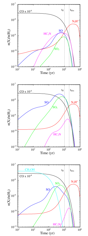
Figure 7: Abundances versus time for selected species. The vertical dotted lines mark the time-scales for gravitational collapse ($t_{\rm ff}$) and clump dissipation ($t_{\rm diss}$). Top: type I cores (no ice sublimation). Middle: type II cores (CO₂ and H₂S sublimation). Bottom: type III cores (CO₂, H₂O, and CH₃OH sublimation).

Figure 7 shows the time evolution of each of the four observed species – CO, SO, HC₃N, and CH₃OH – in each clump. Also shown are N₂H⁺ and SO₂. The free-fall time, $t_{\rm ff}$, and the clump dissipation time, $t_{\rm diss}$ are marked on each panel. In all cases, molecules are depleted from the gas on a freeze-out timescale of a few $\times 10^{5}$ yr. For type I clumps, SO and HC₃N are produced by chemical reactions in the dense gas, peaking between $5\times 10^{4}$ and $10^{5}$ yr. SO is formed via the reaction of atomic S with OH, and HC₃N from ${\rm CN+C_{2}H_{2}}$. Type I clumps younger than $\sim 10^{5}$ yr can account for regions with both SO and HC₃N emission but no methanol. At longer times, SO is destroyed faster than HC₃N, so long-lived clumps of this type are able to explain those regions which are HC₃N-rich but SO-poor. In type II clumps, the injection of H₂S significantly enhances the amount of SO produced in the gas. Compared to type I clumps, the HC₃N peak is slightly reduced, and shifted to later times. This is due to the reduced hydrocarbon abundances which result from the fact that the injected CO₂ drives down the C⁺ abundance. Type II cores can explain regions with large SO abundances, together with small HC₃N abundances and no CH₃OH. Type III clumps are obviously the only ones which can explain CH₃OH-rich clumps, but we find that the methanol only survives for $\sim 10^{4}$ yr before it is destroyed by protonation followed by dissociative recombination. The HC₃N in these clumps only peaks after all the CH₃OH has been lost, which naturally explains the anti-correlation between methanol and cyanoacetylene. The SO abundances in type III clumps are intermediate between those of types I and II, and peaks occur at around $2\times 10^{4}$ yr. At this time, much of the initial CH₃OH has been destroyed, and no significant amounts of HC₃N have been formed. Therefore, type III cores younger than $\sim 10^{4}$ yr will contain both CH₃OH and SO, whereas slightly older cores will only contain SO. Because the injected water leads to an increased OH abundance in the gas, type III cores eventually evolve to a state with ${\rm SO_{2}/SO>1}$, so the SO/SO₂ ratio may potentially be used to place more firm constraints on the ages of these clumps [c.f. 68, 69].

4.4 Application to Observations

We can compare our model results with the observational dataset, to try to place constraints on the ages and the dynamical states of specific objects. Considering the general trends described in section 3.2, we find that our model naturally accounts for the CH₃OH–HC₃N anti-correlation. Clumps with CH₃OH emission must have ages of $t\lower 3.01385pt\hbox{$\buildrel<\over{\sim}\ $}10^{4}$ yr, and those with no SO emission must be even younger ($t\lower 3.01385pt\hbox{$\buildrel<\over{\sim}\ $}5\times 10^{3}$ yr). Because these ages are much less than those associated with the dynamical evolution of the clumps, the dynamical state of methanol clumps cannot be constrained from the observations. As these type III clumps evolve, they eventually lose all the initial methanol; for $3\times 10^{4}\lower 3.01385pt\hbox{$\buildrel<\over{\sim}\ $}t\lower 3.01385pt\hbox{$\buildrel<\over{\sim}\ $}10^{5}$ yr, they will appear only in SO, after which time the HC₃N abundance rises. The evolution of type III clumps provides a simple explanation for the observed transition from pure-CH₃OH to mixed-CH₃OH-SO to pure-SO gas in different velocity channels. Clumps with both SO and HC₃N emission could be old type II or III ($t>10^{5}$ yr), or possibly younger type I clumps. Regions containing only HC₃N emission are likely to be old type I clumps, with ages $t\sim 2\times 10^{5}~{}{\rm yr}\sim t_{\rm diss}$. As these latter clumps have ages comparable to t_diss, it is probable that pure HC₃N clumps represent long-lived, stable clumps: gravitationally bound against dissipation, but not collapsing. If so, then some of these regions should also be associated with enhanced N₂H⁺ abundances, as we in fact see in L1512.

We now briefly consider each source in turn:

L1512

The strong CH₃OH and SO clump in the northwest must have an age of $\sim 10^{4}$ yr. In contrast, the SO cores toward the southeast have only weak methanol emission and must be older. This SO emission surrounds the HC₃N peak which must be even older, as no SO is seen at this position, suggesting an age of $\sim 2\times 10^{5}$ yr. This is consistent with the CO depletion and N₂H⁺ emission also seen toward this position [37]

TMC-1C

The methanol clumps in this source have only weak SO emission, and so must be $t\lower 3.01385pt\hbox{$\buildrel<\over{\sim}\ $}5000$ yr. The clumpy ring of material to the southeast has little or no methanol, but SO and HC₃N are somewhat co-mingled. This is best explained by type I clumps, implying that the mechanism which formed the clumpy ring was not energetic enough to cause significant desorption of grain mantles.

L1262

In this source, the channel velocity maps at 4.12 km s^-1 show a clumpy ring of SO emission surrounding the HC₃N peak. As is the case in L1512 these may represent evolved type III clumps which have lost the original methanol. The central HC₃N clump will be older ($t\lower 3.01385pt\hbox{$\buildrel>\over{\sim}\ $}10^{5}$ yr) than the surrounding SO clumps ($3\times 10^{4}<t<10^{5}$ yr). Both CO clumps in this source display the kinematical sequence of SO followed by SO plus CH₃OH, followed by only CH₃OH, that is typical of the time evolution of type II clumps.

Per 7

Again, we see a transition in velocity space from pure SO to pure CH₃OH via mixed gas. As in L1262, this indicates the evolution of clumps where CH₃OH ice is liberated along the line of sight. The HC₃N peak toward the northeast is associated with weak SO, and may represent evolved gas. However, the peak does not appear to be correlated with the N₂H⁺ peak or with significant CO depletion.

L1389

Again, we see SO-rich gas surrounding a HC₃N-rich region. As in L1512, this suggests an older, stable clump in the center surrounded by regions in which clump formation and/or ice mantle sublimation occurred more recently. This source also shows a clear HC₃N-CH₃OH anti-correlation.

L1251E

SO is only visible in this map toward the north and east, and appears to be associated with some CH₃OH, implying an age for this gas of $\sim 10^{4}$ yr. Towards the south and west, CH₃OH and HC₃N clumps are prevalent yet SO is absent, which requires the presence of both young and old cores. This is the only area in which we see co-mingling of HC₃N and CH₃OH emission – although the peak positions are offset – and is the only region whose chemistry is not readily explained by our simple model.

5 Conclusions

We have mapped several prestellar and protostellar cores in CH₃OH, HC₃N, SO and C¹⁸O. We find that the emission from these molecules traces clumpy structure across all of the cores. The molecular clumps show striking differences in the location and velocity of emission peaks between molecules.

We see a similar degree of chemical differentiation in all of the cores that we have observed, despite the differences in known star forming activity. The HC₃N clumps are generally anti-correlated with N₂H⁺ peaks, and with CH₃OH clumps. In L1512, a HC₃N clump does appear along with a N₂H⁺ peak, perhaps indicative of ongoing molecular depletion. CH₃OH clumps and SO clumps also show distinct emission peaks. C¹⁸O clump peaks are not generally correlated with emission peaks in any of the other molecules that we observed. These morphological differences in molecular peaks towards sources of different evolutionary stage suggest that depletion is important, but that other processes must also be driving the chemical differentiation that we see.

Our observations suggest there is a kinematic sequence through the clumps of different molecular species within the core. There is a well defined emission sequence in velocity space where we see only clumps of SO, then clumps where SO and CH₃OH are intermingled, and then a region with CH₃OH only. This may indicate that we are looking down a cylinder, or filament.

We have investigated the origin of the chemical differentiation using a simple chemical model, in which clumps form rapidly and in which sublimation of ice mantles can occur as the clump is formed. Despite its simplicity, this model is able to account for a wide variety of the chemical differentiation observed in our sources. For clumps in which CH₃OH is injected, the methanol survives for $\sim 10^{4}$ yr, so the observed CH₃OH-rich clumps are young compared to the time-scale for dynamical evolution. In these clumps, HC₃N is not produced until all the CH₃OH has been destroyed, which explains the observed anti-correlation of methanol and cyanoacetylene. The model also predicts some some regions will have ${\rm\hbox{HC${}_{3}$N}/SO}>1$ whereas others will have ${\rm\hbox{HC${}_{3}$N}/SO}<1$, depending on the age of the source and/or the degree of mantle sublimation. HC₃N peaks at late times, and the observed regions with only HC₃N emission are most likely tracing older clumps which are dynamically stable against both collapse and dissipation. Such regions should also be associated with marked CO depletion and elevated N₂H⁺ abundances.

In conclusion, it appears that molecular clouds containing protostars at different epochs of star formation exhibit similar trends in their chemical spatial differentiation. The origin of this differentiation can be understood through simple models of the molecular gas-grain interaction, and suggests that periodic removal of ice mantles is occurring in dark clouds. Mantle disruption and dark cloud chemistry are probably closely connected to the physics of clump evolution, dynamical-chemical models incorporating of these processes are currently being developed [59].

Table 3: Summary of Onsala Observations and Data Analysis

Source	Offset	C18O					CH3OH					HC3N					SO
	(′′)	$\int T_{\rm A}^{*}dv$	$\Delta v$	$V_{\rm LSR}$	$N^{\dagger}$		$\int T_{\rm A}^{*}dv$	$\Delta v$	$V_{\rm LSR}$	$N^{\dagger}$		$\int T_{\rm A}^{*}dv$	$\Delta v$	$V_{\rm LSR}$	$N^{\dagger}$		$\int T_{\rm A}^{*}dv$	$\Delta v$	$V_{\rm LSR}$	$N^{\dagger}$
		(Kkm s-1)	(km s-1)	(km s-1)	($\rm 10^{15}cm^{-2}$)		(Kkm s-1)	(km s-1)	(km s-1)	($\rm 10^{14}cm^{-2}$)		(Kkm s-1)	(km s-1)	(km s-1)	($\rm 10^{12}cm^{-2}$)		(Kkm s-1)	(km s-1)	(km s-1)	($\rm 10^{13}cm^{-2}$)
Per7
	-90,-60	1.77(.07)	0.85(.04)	6.26(.02)	5.43		0.31(.03)	0.52(.03)	6.44(.02)	2.82		0.13(.03)	0.64(.17)	6.38(.07)	0.96		0.93(.07)	0.95(.09)	6.30(.03)	2.32
	-60,0	1.80(.07)	0.72(.04)	6.32(.01)	5.51		0.37(.03)	0.57(.03)	6.53(.02)	3.41		$<$0.01	..	..	$<$0.09		0.75(.07)	0.91(.11)	6.41(.04)	1.86
	-30,30	2.32(.07)	0.87(.03)	6.52(.01)	7.11		0.22(.02)	0.49(.03)	6.68(.02)	2.04		0.09(.01)	0.20(.03)	6.81(.01)	0.68		0.83(.06)	0.68(.06)	6.53(.03)	2.07
	30,0	1.96(.06)	0.75(.03)	6.53(.01)	6.01		0.25(.02)	0.50(.03)	6.68(.02)	2.26		$<$0.01	..	..	$<$0.09		0.53(.07)	0.61(.10)	6.61(.03)	1.31
	30,30	2.30(.06)	0.81(.03)	6.54(.01)	7.03		0.17(.03)	0.44(.03)	6.66(.03)	1.60		0.11(.01)	0.26(.03	6.72(.02)	0.79		0.84(.07)	0.81(.08)	6.55(.03)	2.10
	90,90	2.17(.06)	0.78(.02)	6.62(.01)	6.64		0.43(.04)	0.71(.04)	6.69(.00)	3.93		$<$0.02	..	..	$<$0.11		0.68(.06)	0.64(.07)	6.47(.03)	1.70
L1389
	-60,-30	0.17(.03)	0.37(.06)	-4.81(.04)	0.51		0.11(.03)	0.37(.09)	-4.60(.05)	1.00		0.15(.04)	0.61(.22)	-4.81(.08)	1.11		$<$0.02	..	..	$<$0.04
	-30,-30	0.33(.04)	0.40(.05)	-4.78(.03)	1.01		0.14(.02)	0.29(.02)	-4.64(.01)	1.25		0.27(.02)	0.34(.03)	-4.72(.01)	1.91		0.19(.03)	0.29(.05)	-4.85(.02)	0.47
	-30,0	0.45(.05)	0.59(.07)	-4.81(.04)	1.38		0.11(.03)	0.48(.08)	-4.69(.05)	1.05		0.29(.02)	0.33(.02)	-4.67(.01)	2.07		0.25(.03)	0.36(.04)	-4.85(.02)	0.62
TMC-1C
	-90,120	1.50(.09)	0.43(.03)	5.07(.01)	4.59		0.29(.03)	0.25(.02)	5.28(.01)	2.64		$<$0.03	..	..	$<$0.23		0.50(.08)	0.85(.14)	5.31(.0)8	1.24
	-60,60	1.38(.09)	0.42(.03)	5.12(.01)	4.21		0.50(.03)	0.33(.01)	5.33(.01)	4.58		0.15(.02)	0.22(.03)	5.25(.02)	1.06		0.32(.04)	0.29(.04)	5.13(.02)	0.79
	-30,-60	1.48(.11)	0.47(.05)	5.24(.02)	4.54		0.23(.04)	0.30(.03)	5.38(.02)	2.16		0.33(.03)	0.26(.03)	5.31(.01)	2.35		0.25(.04)	0.17(.03)	5.15(.01)	0.63
	-30,30	1.30(.08)	0.33(.02)	5.16(.01)	3.97		0.48(.03)	0.32(.01)	5.33(.01)	4.42		0.31(.03)	0.21(.02)	5.24(.01)	2.22		0.45(.06)	0.44(.08)	5.22(.03)	1.13
	30,-30	1.35(.08)	0.37(.02)	5.16(.01)	4.12		0.30(.01)	0.30(.08)	5.30(.08)	2.79		0.24(.03)	0.26(.05)	5.08(.02)	1.72		0.38(.05)	0.32(.05)	5.12(.02)	0.94
L1512
	-60,-30	0.65(.04)	0.31(.02)	7.02(.01)	2.00		0.14(.02)	0.29(.03)	7.21(.02)	1.25		0.19(.03)	0.21(.04)	7.07(.02)	1.33		0.14(.03)	0.28(.08)	7.09(.04)	0.34
	-60,120	0.38(.04)	0.25(.03)	6.86(.01)	1.18		0.35(.02)	0.31(.01)	6.97(.01)	3.20		0.09(.02)	0.11(.02)	7.59(.01)	0.67		0.42(.03)	0.31(.03)	6.85(.0)1	1.05
	-30,-30	0.42(.04)	0.22(.0)2	7.02(.01)	1.29		0.16(.02)	0.25(.01)	7.21(.01)	1.44		0.29(.02)	0.17(.02)	7.08(.01)	2.05		0.57(.07)	1.13(.17)	7.05(.0)7	1.43
	-30,0	0.42(.03)	0.22(.02)	7.08(.01)	1.28		0.18(.02)	0.25(.02)	7.21(.01)	1.67		0.48(.03)	0.24(.02)	7.09(.01)	3.41		$<$0.03	..	..	$<$0.07
L1251E
	-210,0	2.63(.17)	1.41(.11)	-3.81(.05)	8.06		0.95(.05)	1.24(.03)	-3.88(.03)	8.70		0.73(.05)	0.97(.08)	-3.67(.03)	5.27		$<$0.02	..	..	$<$0.06
	-180,0	1.71(.16)	1.40(.15)	-3.76(.07)	5.23		0.95(.07)	1.84(.08)	-3.97(.05)	8.72		0.58(.05)	0.76(.09)	-3.40(.03)	4.17		$<$0.03	..	..	$<$0.07
	-150,0	1.58(.15)	1.25(.12)	-3.72(.06)	4.83		0.77(.05)	1.11(.05)	-3.68(.04)	7.04		0.85(.05)	0.59(.04)	-3.43(.01)	6.07		0.80(.09)	1.46(.19)	-3.77(.0)8	1.99
	-120,120	0.96(.08)	0.82(.08)	-4.38(.03)	2.93		0.57(.07)	1.18(.09)	-4.16(.07)	5.22		$<$0.02	..	..	$<$0.16		2.04(.08	1.08(.05)	-4.36(.02)	5.07
	-90,60	1.72(.10)	1.02(.07)	-4.16(.03)	5.28		1.10(.08)	1.73(.08)	-4.21(.06)	10.05		0.17(.03)	0.27(.05)	-3.77(.02)	1.24		1.39(.08)	1.22(.09)	-4.67(.04)	3.47
L1262
	0,0	1.01(.07)	0.51(.04)	3.82(.02)	3.08		0.43(.02)	0.39(.01)	3.98(.01)	3.93		0.19(.01)	0.40(.04)	3.89(.01)	1.36		0.56(.04)	0.51(.04)	3.77(.02)	1.40
	0,30	0.86(.07)	0.58(.06)	3.85(.02)	2.64		0.62(.03)	0.51(.01)	4.02(.01)	5.72		0.28(.02)	0.38(.03)	3.85(.02)	1.99		1.10(.05)	0.64(.03)	3.85(.01)	2.74
	30,-30	0.64(.06)	0.45(.06)	3.96(.02)	1.95		0.28(.02)	0.47(.02)	4.11(.02)	2.57		0.20(.02)	0.35(.06)	4.04(.02)	1.44		0.42(.05)	0.48(.07)	4.04(.03)	1.05
	60,-30	1.11(.08)	0.74(.07)	4.10(.03)	3.40		0.42(.03)	0.60(.03)	4.33(.02)	3.90		0.30(.03)	0.53(.05)	4.06(.02)	2.16		0.68(.05)	0.62(.05)	4.08(.02)	1.70

NOTE: The error estimate in parenthesis is the 1$\sigma$ error estimate. Upper limits are 3$\sigma$. For column densities, upper limits are based on $T_{\rm A}^{*}$$\Delta$v, where the value of $\Delta$v is the channel width, and $T_{\rm A}^{*}$ is taken to be 3 $\sigma$.
^† see text for details

References

- [1] Shu F.H., Adams F.C. & Lizano S., 1987 ARA&A, 25,23
- [2] Mac Low M.-M.& Klessen R. S. 2004, Rev. Mod. Phys., 76, 125
- [3] Hartmann L., Ballesteros-Paredes J, & Bergin E. A. 2001, ApJ, 562, 852
- [4] Evans N.J. II, 1999, ARA&A 37, 311
- [5] Benson P. J., & Myers P.C., 1989 ApJS 71, 89
- [6] Peng R., Langer W.D., Velusamy T., Kuiper T.B.H. & Levin S., 1998, ApJ 497, 842
- [7] Takakuwa, S., Mikami, H., Saito, M., & Hirano, N., 2000, ApJ 542, 367
- [8] Takakuwa S., Kamazaki T., Saito M. & Hirano N., 2003, ApJ 584, 818
- [9] Swade D.A, 1989, ApJ 345 828
- [10] Pratap P., Dickens J.E., Snell R.L., Miralles M.P., Bergin E.A., Irvine W.M. & Schloerb F.P., 1997, ApJ 486, 862
- [11] Dickens J.E., Irvine W.M., Snell R.L., Bergin E.A., Schloerb F.P., Pratap P. & Miralles M.P., 2000, ApJ 542, 870
- [12] Olano, C., Walmsley, C.M. & Wilson, T.L. 1988, A&A 196, 194
- [13] Turner B.E., 2001, ApJS 136, 579
- [14] Hirota T., Ikeda M.& Yamamoto S., 2001, ApJ 547, 814
- [15] Morata O., Girart J.M., Estalella R., 2003, A&A 397, 181
- [16] Tafalla M., Santiago J. 2004, A&A 414, L53
- [17] Bergin E. A., Alves J., Huard T., Lada, C.J., 2002, ApJ 570, L101
- [18] Caselli P., van der Tak F.F.S., Ceccarelli, C. & Bacmann A., 2003, A&A 403, L37
- [19] Scalo J. & Elmegreen B.G., 2004, ARA&A 42, 275
- [20] Elmegreen B.G. & Scalo J., 2004, ARA&A 42, 275
- [21] Reipurth B. & Bally J., 2001, ARA&A 39, 403
- [22] Norman C. & Silk J. 1980, ApJ, 238, 138
- [23] Walawender J., Bally J. & Reipurth B., 2005, AJ 129, 2308
- [24] Quillen A.C., Thorndike S.L., Cunningham A., Frank A., Gutermuth R.A., Blackman E.G., Pipher J.L., Ridge N., 2005, ApJ 632, 941
- [25] Motte F., Andre P. & Neri, R., 1998, A&A 336, 150
- [26] Charnley S.B., Dyson J.E., Hartquist T.W. & Williams D.A., 1988, MNRAS 235, 1257
- [27] Suzuki H., Yamamoto S., Ohishi M., Kaifu N., Ishikawa S., Hirahara Y. & Takano S., 1992, ApJ 392, 551
- [28] Aikawa Y., Herbst E., Roberts H., Caselli P., 2005, ApJ 620, 330
- [29] Markwick, A.J., Millar, T.J. & Charnley S.B., 2000, ApJ, 535, 256
- [30] Charnley S.B., Rodgers S.D., Ehrenfreund P., 2001, A&A 378, 1024
- [31] Garrod R.T., Williams D.A., Hartquist T.W., Rawlings J.M.C., Viti S., 2005, MNRAS 356, 654 (Erratum : 362, 749)
- [32] Goldsmith P.F., Langer W.D., Wilson R.W., 1986, ApJ 303, L11 Langer, W. D., & Wilson, R. W., 1986, ApJ 303, L11
- [33] Fuller, G. A., Myers, P. C., Welch, W. J., Goldsmith, P. F., Langer, W. D., Campbell, B. G., Guilloteau, S. & Wilson, R. W., 1991, ApJ 376, 135
- [34] Kelly M.L., MacDonald G.H., Millar T.J., 1996, MNRAS 279, 1210
- [35] Charnley S.B. et al. 2006, ApJ submitted
- [36] Butner H.M. et al. 2006, ApJ, submitted
- [37] Caselli P., Bensen P.J., Myers P.C. & Tafalla M., 2002, ApJ 572, 238
- [38] Schnee S. & Goodman A., 2005, ApJ 632, 1168
- [39] Cernicharo J., Guelin M., Askne J., 1984, A&A 138, 371
- [40] Laundhardt R. & Henning T. 1997, A&A 326, 329
- [41] Shirley, Y.L., Evans Neal J., II, Rawlings J.M.C., Gregersen E.M., 2000, ApJS 131, 249
- [42] Kun M. & Prusti T., 1993, A&A 272, 235
- [43] Ehrenfreund P. & Charnley S.B., 2000, ARA&A 38, 427
- [44] Geppert W.D. et al., 2006, in Astrochemistry Throughout the Universe: Recent Successes and Current Challenges, eds. D.C. Lis, G.A. Blake & E. Herbst, Cambridge University Press, in press
- [45] Ruffle, D. P., Hartquist, T. W., Caselli, P. & Williams, D. A., 1999, MNRAS 306, 691
- [46] Millar T.J. & Herbst E., 1990, A&A, 231, 466
- [47] Palumbo, M.E., Geballe, T.R. & Tielens A.G.G.M., 1997, ApJ 479, 839
- [48] Thompson M.A., MacDonald G.H. & Millar T.J., 1999, A&A 342, 809
- [49] Pickett H.M., Poynter R.L., Cohen E.A., Delitsky M.L., Pearson J.C., and Muller H.S.P., 1998, J. Quant. Spectrosc. & Rad. Transfer 60, 883
- [50] Schöier F.L., van der Tak F.F.S., van Dishoeck E.F., Black J.H., 2005, A&A 432, 369
- [51] Cragg, D.M., Mikhtiev, M.A., Bettens, R.P.A., Godfrey, P.D., & Brown, R.D., 1993, MNRAS 264, 769
- [52] Menten K.M., Walmsley C.M., Henkel C., & Wilson T.L., 1986, A&A 157, 318
- [53] Kalenskii S.V., Dzura, A.M., Booth R.S., Winnberg A., Alakoz A.V., 1997, A&A 321, 311
- [54] Frerking M.A., Langer W.D. & Wilson R.W., 1982, ApJ 262, 590
- [55] Ruffle D.P., Hartquist T.W., Taylor S.D. & Williams D.A., 1997, MNRAS 291, 235
- [56] Klessen R.S., 2001, ApJ, 556, 837
- [57] Brown P.D. & Charnley S.B., 1990, MNRAS 244, 432
- [58] MacLaren I., Richardson K.M. & Wolfendale A.W., 1988, ApJ 333, 821
- [59] Rodgers, S.D. et al. 2006, in preparation.
- [60] Rodgers S.D. & Charnley S.B., 2001, ApJ, 546, 324
- [61] Geppert W.D. et al., 2004, ApJ, 609, 459
- [62] Geppert W.D. et al., 2004, ApJ, 610, 1228
- [63] Geppert W.D. et al., 2005, ApJ, 631, 653
- [64] Kalhori S. et al., 2002, A&A, 391, 1159
- [65] Dickens J.E., Langer W.D., Velusamy T., 2001, ApJ, 558, 693
- [66] Knez C. et al., 2005, ApJL, 635, L145
- [67] Aikawa Y., Umebayashi T., Nakano T., Miyama S.M., 1997, ApJ, 486, L51
- [68] Charnley S.B., 1997, ApJ, 481, 396
- [69] Buckle J.V. & Fuller G.A., 2003, A&A, 399, 1047