Optimization in Gradient Networks

Abstract

Gradient networks can be used to model the dominant structure of complex networks. Previous works have focused on random gradient networks. Here we study gradient networks that minimize jamming on substrate networks with scale-free and Erdős-Rényi structure. We introduce structural correlations and strongly reduce congestion occurring on the network by using a Monte Carlo optimization scheme. This optimization alters the degree distribution and other structural properties of the resulting gradient networks. These results are expected to be relevant for transport and other dynamical processes in real network systems.

Complex networks have been shown to offer a powerful framework for the study of dynamical processes in complex systems general_1 ; general_2 . A fundamental question in this context is to identify how the structure of dominant connections influences the dynamical properties of the entire system. Gradient networks have been introduced in references zoltan ; zoltan2 precisely to characterize the structure governing transport in complex networks. Remarkably, similar structures have been identified recently in the optimization of synchronizability in oscillator networks grad_application1 ; grad_application2 . Here, we consider the problem of optimization of transport and show that by using a Monte Carlo approach congestion can be reduced in complex networks. We discuss the structural correlations that emerge with optimization and its implications for real systems.

I Introduction

The efficiency of transport systems has been of interest in various fields, including physics, biology and engineering. In transport processes, the item being transported usually follows the steepest descent of the underlying surface, e.g., water flowing down the slopes of a mountain. Flow in networks has been modeled by Toroczkai et al. zoltan ; zoltan2 by the introduction of local gradients on a substrate network. The gradient network defined on this network has provided significant insights into the dominant structures that provide transport efficiency. They have considered a fixed network of $N$ nodes with a scalar potential, $V_{i}$ at each node $i$. The gradient $\nabla V_{i}$ of the potential at each node $i$ is a directed edge which points from $i$ to the neighbor with the minimum potential among all the neighbors of $i$.

Toroczkai et al have shown several properties of gradient networks which we briefly summarize. An interesting topological property of the gradient network is that its in-degree distribution is scale-free for both scale-free (SF) and Erdős-Rényi (ER) substrate networks general_2 . A gradient network with a non-degenerate potential distribution, is a group of trees, hence no loops exist in this network other than self-loops. Only this property makes the gradient networks very common in seemingly unrelated problems, i.e., synchronization in oscillatory networks grad_application1 ; grad_application2 . The relationship between network topology and congestion has also been investigated zoltan ; zoltan2 by introducing a measure of congestion, the jamming coefficient. This measure involves the ratio of the number of nodes that receive at least one gradient link, $N_{\rm receive}$ and the number of nodes that send a link. By definition, every node sends one out link, therefore the number of senders in the network, $N_{send}=N$. The jamming coefficient is

$$J=1-\left\langle\!\left\langle N_{\rm receive}/N_{\rm send}\right\rangle_{V}\right\rangle_{\rm network}.$$ (1)

The operations $\langle\ldots\rangle_{V}$ and $\langle\ldots\rangle_{\rm network}$ denote the statistical averaging over local potentials and networks respectively. Maximal congestion occurs at $J=1$, and no congestion occurs when every link receives a gradient link, corresponding to $J=0$. It was also found that $J$ is independent of number of nodes $N$ for scale free substrate network, and these networks are not prone to maximal jamming. The jamming coefficient was extensively studied by Park et al. park where they compared it for ER and SF networks with the same average degree, $\langle k\rangle$, for $2<\langle k\rangle<200$. With randomly assigned potentials on each node, below $\langle k\rangle\approx 10$, they found that ER networks are less congested than SF networks.

Here we introduce a Monte Carlo optimization scheme that reduces jamming significantly and introduces structural correlations into the system that are not built in. The remainder of the paper is organized as follows. In Section II we introduce the algorithm for optimizing jamming coefficient that is initially calculated from randomly assigned scalar values at each node. We compare the optimized jamming values of a scale-free network and an Erdős-Rényi network for various values of average degrees. In Section III we investigate the structure of the optimal gradient network. In particular we study the degree distribution and the correlations between the degree and the potential of each node. Finally in Section IV we discuss the implications and the possible extensions of optimal gradient networks.

II Optimization of Jamming

Previous work  zoltan ; zoltan2 has focused on random gradient networks where the potential on each node has a randomly assigned value. More generally, the potentials can be a dynamic quantity evolving in time due to perturbations, sources and sinks internal and external to the system of interest. Alternatively, the potentials can evolve to become correlated to the network properties such as its degree distribution. For example, consider the networks of routers where every router has a capacity. If a router is central and highly connected, it usually has a higher capacity in order to handle the traffic en-route effectively. Recently, a congestion aware routing algorithm has been introduced where the transport on the network of routers is driven by congestion-gradients danila .

Here we develop a Monte Carlo algorithm to achieve two goals: reduce jamming in the network, and observe the emerging optimal correlation between in-degree and potential of each node. For a given network and potential distribution, we redefine J in Eq. 1 as $J=1-N_{\rm receive}/N$ where $N_{\rm send}=N$ by definition. The initial potential distribution is chosen from a Gaussian distribution, and at each iteration the potential of a random node is modified such that global congestion is reduced. We use a Metropolis algorithm barkema with the following steps:

1. Pick a node, $i$ at random.

2. Vary $V_{i}$ by $\delta V$, i.e., ${V_{i}}_{\rm new}=V_{i}+\delta V$ where $\delta V$ is a Gaussian random variable with variance $\sigma^{2}=1$.

3. Recalculate $J$ with ${V_{i}}_{\rm new}$.

4. Accept ${V_{i}}_{\rm new}$ with probability $p\sim\exp[-\Delta J/T]$ where $\Delta J=J_{\rm new}-J_{\rm old}$.

5. Go to step 1, and repeat.

The fictitious temperature, $T$ is chosen to adjust the acceptance ratio to about 40%. We perform the optimization procedure until $J(t)$ equilibrates, i.e., at large $t$ the time autocorrelation function of $J(t)$ gould ,

$$C_{J}(t)=\frac{[\langle J(t)J(0)\rangle-\langle J\rangle^{2}]}{[\langle J^{2}\rangle-\langle J\rangle^{2}]},$$ (2)

goes to zero.

Using the described optimization algorithm, we can significantly reduce the jamming coefficient in both SF and ER networks. Following previous work zoltan ; park we choose as the SF network a Barabási-Albert model general_2 ; science . For this network the average connectivity is $\langle k\rangle=2m$ where each node has at minimum $m$ links. The network size throughout the paper is chosen to be $N=10000$. For the ER networks, $\langle k\rangle=pN$ where $p$ is the probability of having a link between any pair of nodes. We use the same $\langle k\rangle$ when comparing the two types of network by adjusting $m$ and $p$. The evolution of jamming coefficient during optimization is shown in Fig. 1 as a function of algorithmic time in units of Monte Carlo steps (mcs) for $\langle k\rangle=4$. At $t=0$ (see also inset of Fig. 1), the SF network has a higher jamming coefficient, but after roughly 50000 mcs, the SF network becomes less congested compared to the ER network. The initial and final jamming coefficients for the two networks are ${J_{i}}_{SF}=0.57$, ${J_{i}}_{ER}=0.52$, ${J_{f}}_{SF}=0.31$, and ${J_{f}}_{ER}=0.36$, respectively.

Figure 1: Optimized jamming, $J(t)$, as a function of time in Monte Carlo steps (mcs) for SF ($\bullet$) and ER ($\circ$) networks with the same average degree, $<k>=4$ and $N=10000$. As shown in the inset, SF network with random potential distribution has a higher jamming coefficient at $t=0$ compared to the ER network. After optimization is completed, however, optimal SF network has a lower jamming coefficient.

We define $\Delta J_{r}$ and $\Delta J_{o}$, the difference in jamming between SF and ER networks for random and optimal networks respectively. For a given network with $\langle k\rangle$, $\Delta J_{r}$ is calculated initially at $t=0$ and $\Delta J_{o}$ at $t_{\rm opt}$ after optimization is completed, for $2\leq\langle k\rangle\leq 126$. As shown in Fig. 2, $\Delta J_{o}<0$ for $\langle k\rangle>2$ whereas $\Delta J_{r}>0$ indicating that SF networks have a lower jamming coefficient after optimization, a result significantly different than those for random gradient networks park .

Figure 2: Difference between the jamming values of SF and ER networks, $\Delta J=J_{SF}-J_{ER}$ for various $\langle k\rangle$ for random ($\circ$) and optimal ($\bullet$) gradient networks. $\Delta J<0$ for all simulated $\langle k\rangle>2$ indicating that optimal SF networks have a lower jamming coefficient than optimal ER networks.

III Structural Properties of Optimal Networks

As shown in Fig. 1 congestion can be reduced in gradient networks by varying the potentials at each node. It is reasonable to expect that the obtained optimal potentials may also alter the structure of the gradient network. Next, we analyze the structural properties of optimal gradient networks such as the degree distribution. Previously, the random gradient network of an ER substrate network was shown numerically and analytically zoltan ; zoltan2 to have an in-degree distribution of $R(l)\sim l^{-1}$. However, the SF substrate network with degree distribution $P(k)\sim k^{-3}$, was shown to have a gradient degree distribution of $R(l)\sim l^{-3}$.

The degree distribution of the random and optimal ER and SF networks are shown for $p=0.001$ ($\langle k\rangle=10$) and $m=3$ ($\langle k\rangle=6$) respectively in Figure 3 along with the expected scaling exponents for the random gradient networks of $-1$ and $-3$. The statistical averaging is obtained over 100 networks. For ER networks, the scaling region extends with higher average connectivity, however we chose to use a small $\langle k\rangle=10$ for which optimization is more efficient. The optimization is performed for 1 million Monte Carlo steps. The jamming values initially are 0.62, 0.71 and after optimization reduce to 0.36, 0.60 for SF and ER respectively. The in-degree distribution, $R(l)$, for the SF network varies significantly with the optimization. The cut-off degree is reduced an order of magnitude (from roughly 100 to 10) compared to the random one, and the scaling is now steeper. On the other hand, the ER network does not show a major change in the degree distribution.

Figure 3: In-degree distributions, $R(l)$, for gradient networks of (a) SF and (b) ER networks with $m=3$ and $p=0.001$ respectively before ($\circ$) and after ($\bullet$) optimization of jamming. The dashed lined indicates the scaling of $R(l)\sim l^{\alpha}$ from Ref. zoltan ; zoltan2 , where $\alpha=-3$ and $-1$ for random SF and ER networks respectively. The scaling exponent $\alpha$ is not a good fit for optimal SF data but a good fit for optimal ER network.

Next, we analyze the probability distribution of potentials for nodes in the substrate networks with degree $k$, before and after the optimization to observe any degree-potential correlations. The results are shown in Fig. 4 for the SF network ($m=3$). To reduce noise in the data especially for large values of $k$, the degrees are binned into four groups: $3<k\leq 10$, $10<k\leq 30$, $30<k\leq 50$, $50<k\leq 100$. Before optimization with initial random Gaussian potentials within range [-4, 4] , each set has the same probability distribution $P(V_{i})$ as shown in the inset of Fig 4. This behavior is expected as no correlation was built in between the degree of a node and its potential. After the optimization however, the range of the potentials has broadened significantly, and the nodes with high degree have accumulated very large potentials.

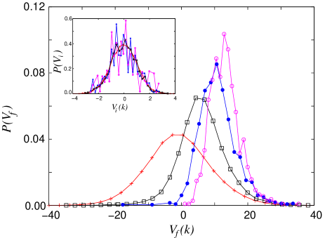
Figure 4: Probability distribution of the potentials of nodes with degree $k$ for SF network with $m=3$ before (inset) and after optimization. The degrees are binned to indicate the correlation between degree of a node and its potential: $3<k\leq 10$ ($+$), $10<k\leq 30$ ($\square$), $30<k\leq 50$ ( $\bullet$), $50<k\leq 100$ ( $\circ$). Before the optimization $P(V_{i})$ do not show any correlations with $k$, however after the optimization, nodes with high degree, get the large values of potential which facilitates reduced jamming.

With the improved jamming coefficient, it is natural to expect some correlation to emerge between the potential of the node and its degree. If the node has a large degree and a small potential, this node will be preferred by most of its neighbors for sending an out link, and thus this will contribute to higher jamming. However if the potential is large, the neighboring nodes will not prefer this highly connected node and thus not increase the jamming. This intuitive observation implies the possibility of obtaining a reduced congestion by starting with potentials that are inversely correlated with the degree of each node on the substrate network. We tested this case for the SF network ($m=3$) with a correlated potential distribution, $V_{i}=r/k_{i}$ at node $i$ with degree $k_{i}$ where $r$ is a random number chosen from a uniform distribution. This assignment with correlations built-in did not make the jamming coefficient lower. On the contrary it was higher, $J=0.77$, than the value without degree correlation, $J=0.62$.

An interesting observation that Fig. 4 provides is that nodes with small degree carry potentials distributed over a large range $[-40,40]$. For example, nodes with degrees, $3<k<10$ have a roughly Gaussian potential distribution. For higher $k$, the distribution narrows down and shifts toward larger values. For nodes with $50<k<100$, all nodes have large potentials, within range $[0,40]$. This observation might explain why in the test case the jamming was actually higher when the degree was correlated with the potential. In that case, we only assigned low potentials to low degree nodes which still yields congestion much higher than the optimal one. An analytical formulation that distributes the potentials according to its degree mimicking the transitive behavior in Fig. 4 seems possible, but is beyond the scope of this paper.

IV Conclusion

We have introduced a Monte Carlo method to optimize congestion in random gradient networks. Previously the potentials have been assigned randomly and was shown that ER networks had lower jamming coefficient below $\langle k\rangle=10$ than SF networks with the same connectivity park . This was puzzling as the connectivity commonly observed in natural and man-made networks general_2 is usually in this range, but tends to be scale-free, and in scale-free networks jamming is independent of $N$. With the Monte Carlo based optimization scheme we optimized jamming by varying the potentials so that optimal congestion was achieved. We found that optimal SF networks have lower congestion factor for $\langle k\rangle>2$. This reduced congestion is the result of a complex correlation between the degree and the potential of a node. We found that nodes with large degrees in the substrate network get large positive values whereas nodes with small degrees get a Gaussian like distribution of potentials.

Throughout the paper we have used the definition of jamming introduced in Ref. zoltan for a substrate network with unweighted links. A natural extension of this work for generality is to assign weights to links and redefine the jamming coefficient accordingly. A possible definition is $J=\big{(}\sum_{i}\big{[}\sum_{j}w_{ij}-c_{i}\big{]}\big{)}/\sum_{i}c_{i}$ where $i=1\cdots N$, $j$ is the number of neighboring links node $i$ has, $c_{i}$ is the capacity of node $i$, $w_{ij}$ is the weight of the incoming link from j to i, and the operation $[x]=0$ if $x<0$. If the weights and capacity of all nodes are 1, then this definition of $J$ reduces to the one in Eq. 1 without the averaging. With this definition and the optimization method introduced in the paper, it is possible to study real world networks and get insights to the dominant structures of transport for these systems.

- (1) A. E. Motter, M. A. Matias, J. Kurths, and E. Ott, Physica D 224, vii (2006).
- (2) M. E. J. Newman, A.-L. Barabási and D. J. Watts (Editors), The Structure and Dynamics of Networks (Princeton University Press, 2006).
- (3) A.-L. Barabási and R. Albert, Science 286, 509 (1999).
- (4) Z. Toroczkai and K. E. Bassler, Nature 428, 716 (2004).
- (5) Z. Toroczkai, B. Kozma, K. E. Bassler, N. W. Hengartner, and G. Korniss, e-print cond-mat/0408262.
- (6) T. Nishikawa and A. E. Motter Phys. Rev. E 73, 065106 (2006).
- (7) T. Nishikawa and A. E. Motter, Physica D 224, 77 (2006).
- (8) K. Park, Y.-C. Lai, L. Zhao, and N. Ye, Phys. Rev. E 71, 065105 (2005).
- (9) B. Danila , Y. Yu, S. Earl, J. A. Marsh, Z. Toroczkai, and K. E. Bassler, Phys. Rev. E 74, 046114 (2006).
- (10) H. Gould, J. Tobochnik and W. Christian, Introduction to Computer Simulations Methods, Addison-Wesley (2006).
- (11) M. E. J. Newman and G. T. Barkema, Monte Carlo Methods in Statistical Physics, Oxford University Press (1999).