Fluctuations of the partial filling factors in competitive RSA from binary mixtures

Abstract

Competitive random sequential adsorption on a line from a binary mix of incident particles is studied using both an analytic recursive approach and Monte Carlo simulations. We find a strong correlation between the small and the large particle distributions so that while both partial contributions to the fill factor fluctuate widely, the variance of the total fill factor remains relatively small. The variances of partial contributions themselves are quite different between the smaller and the larger particles, with the larger particle distribution being more correlated. The disparity in fluctuations of partial fill factors increases with the particle size ratio. The additional variance in the partial contribution of smaller particle originates from the fluctuations in the size of gaps between larger particles. We discuss the implications of our results to semiconductor high-energy gamma detectors where the detector energy resolution is controlled by correlations in the cascade energy branching process.

I Introduction

One dimensional irreversible random sequential adsorption (RSA) has been of interest for several decades. Its numerous extensions include RSA with particles expanding in the adsorption process Rodg ; viot ; assl , two-size particle adsorption bartelt ; hassan1 ; hassan2 ; Araujo , and also RSA with an arbitrary particle-size distribution function mao . The interest is due to the relevance of this process to a number of physical phenomena in different fields of application, such as information processing coff , particle branching in impact ionization ino and crack formations in crystals under external stress crack . The simplest example of RSA is the so-called car parking problem (CPP). In the context of CPP, one studies the average number of particles (“cars”) adsorbed on a long line and the variance of this number. Equivalently, one is concerned with the distribution function for the size of gaps between the parked cars (see Refs. Talbot ; Privman for the review).

The problem of competitive RSA from a binary mixture is of special interest because of the non-trivial correlations in both the particle and gap-size distributions, developed during the deposition. These correlations manifest themselves in the final irreversible state corresponding to the so-called “jamming limit” — when every gap capable of adsorbing a particle has done so. Numerous studies, reported in the literature for the binary-mixture RSA in the jamming limit, addressed the problem of correlations only indirectly, through its manifestation in the fill factor or the gap distribution. Available results include binary mixtures with point-like particles bartelt ; hassan1 and those with a relatively small particle size ratio, $b/a<2$ hassan2 . Also available are Monte-Carlo studies of the fill factor and the gap-size distribution for a binary-mixture deposition with equal abundance of both particles Araujo .

The present study is concerned with the correlation between the fluctuations in the number of adsorbed particles of each kind from a two-size binary mixture, as well as with their partial contributions to the fill factor. We present both analytical results and those obtained by Monte-Carlo simulations for a wide range of binary-mixture compositions and size ratios.

We are interested in the RSA problem primarily because of its relevance to the propagation of high-energy $\gamma$-particles through a semiconductor crystal — with particle energy branching (PEB) due to cascade multiplication of secondary electrons and holes ino ; Devan ; Spieler ; Klein ; rusb . The correlation of energy distribution between secondaries is quite similar to that of the gap distribution in the RSA process corr . In both cases, the ratio of the variance of the final number of particles to the average particle number in the final (jamming) state can be much less than unity, which is favorable for the detector energy resolution. This ratio (which would be unity if the particle number obeyed a Poisson distribution) is called the Fano factor, $\Phi$ Fano .

The reported attempts to evaluate $\Phi$ employed oversimplified models of the semiconductor band structure. In such models, all crystal properties are characterized by three parameters, namely, the band gap, the phonon frequency, and the ratio of the rate of phonon emission to that of impact ionization. The price of this oversimplification had been that correspondence with experiment could be achieved only by assuming unphysically large rates of phonon losses (about $0.5$ eV per created e-h pair). This does not corroborate with the known values for the ratio of the impact ionization and the phonon emission probabilities for high-energy electrons in semiconductors. The model furthermore obscures the role of features in the band structure and the ionization process that are specific to a particular semiconductor.

In our earlier work assl , we used an extended RSA model of particles that expand or shrink upon adsorption. The shrinking model is relevant to the PEB problem in that it helps to elucidate such factors as the non-constant density of states in the semiconductor band and the fact that due to momentum conservation the ionization threshold is larger than the actual (bandgap) energy that is lost in impact ionization.

The recursive technique employed in Ref. assl allowed us to assess the accuracy of approximate approaches to the yield and variance calculations (such as, e.g., the average-loss approach of Refs. Spieler ; Klein ).

In the present work, the RSA model is extended in a different direction — competitive deposition of different-size particles from a binary mixture — that is suitable to simulate the role of multiple channels of pair production, owing to the multi-valley nature of semiconductor bands. We arrive at a number of qualitative conclusions that should be taken into account in both the interpretation of experimental data and the choice of the crystal composition and device structure in gamma detectors optimized for energy resolution.

The paper is organized as follows. Section II presents the basic equations of the recursive approach and the analytical results for the fill factor and its variance for the larger particles. In Sect. III, we analyze the results that demonstrate high correlation in the particle distribution. Based on the gained understanding, we formulate in Sec. IV the implications of our results for the Fano factor of semiconductor $\gamma$ detectors. Our conclusions are summarized in Sect. V. Certain analytical results are derived in the Appendix.

II Partial contributions to the fill factor and its variance for two-size RSA problem

We consider the problem of competitive deposition from a binary mixture of particles with sizes $a$ and $b$, whose relative contributions to the total flux on the adsorbing line are $q$ and $p=1-q$, respectively. We shall use a recursive approach to first study the mean number of particles $n_{a}(x)$ and $n_{b}(x)$, adsorbed on a line of length $x$ (in the jamming limit), and then the corresponding variances.

Consider a large enough empty length $x>a,b$. We assume that the adsorption is sequential, i.e. only one particle is adsorbed at a time. The first adsorbed particle will be of size $a$ with the probability of landing at any point $q(x-a)/(x-\overline{l})$ or of size $b$ with the landing probability $p(x-b)/(x-\overline{l})$. Here $\overline{l}=qa+pb$ is the “average” particle size in the binary flux. After the first particle is adsorbed, it fills a certain interval $[y,y+a]$ (or $[y,y+b]$), and leaves two independent segments, whose combined size is either $x-a$ or $x-b$. The average numbers of $a$-particles $n_{a}(y)$ and $n_{a}(x-y-a)$ (or $n_{a}(y)$ and $n_{a}(x-y-b)$) will be subsequently adsorbed in these gaps. Thus, the recursion relation is of the form

$$n_{a}(x) = \frac{q(x-a)}{x-\overline{l}}[1+n_{a}(y)+n_{a}(x-a-y)]$$

$$+\frac{p(x-b)}{x-\overline{l}}[n_{a}(y)+n_{a}(x-b-y)]~{},$$

where the first and the second terms (upper and lower lines) correspond to the cases of the first landed particle being a particle of sort $a$ or $b$, respectively. These cases must be averaged over all possible landing coordinates $y$ of the first particle in a different way, viz. for $a$ first,

$$<n_{a}(y)>_{a}=\frac{1}{x-a}\int_{0}^{x-a}n_{a}(y)dy~{},$$

whereas for $b$ first,

$$<n_{a}(y)>_{b}=\frac{1}{x-b}\int_{0}^{x-b}n_{a}(y)dy~{}.$$

Performing the average and using the symmetry between left and right segments we obtain, finally:

$$n_{a}(x) = \frac{q(x-a)}{x-\overline{l}}+\frac{2q}{x-\overline{l}}\int_{0}^{x-a}n_{a}(y)dy$$ (1)

$$+\frac{2p}{x-\overline{l}}\int_{0}^{x-b}n_{a}(y)dy.$$

A similar equation holds for the particles of size $b$:

$$n_{b}(x) = \frac{p(x-b)}{x-\overline{l}}+\frac{2q}{x-\overline{l}}\int_{0}^{x-a}n_{b}(y)dy$$ (2)

$$+\frac{2p}{x-\overline{l}}\int_{0}^{x-b}n_{b}(y)dy.$$

With the help of Eqs. (1,2) one can readily derive an equation for the average total covered length $f(x)$, defined as $f(x)=an_{a}(x)+bn_{b}(x)$, giving

$$f(x) = \frac{x\overline{l}-qa^{2}-pb^{2}}{x-\overline{l}}+\frac{2q}{x-\overline{l}}\int_{0}^{x-a}f(y)dy$$ (3)

$$+\frac{2p}{x-\overline{l}}\int_{0}^{x-b}f(y)dy.$$

Equation (3) agrees with that of Ref. mao for the total covered length in RSA from a multi-size mixture. However, the advantage of Eqs. (1,2) is that they permit studying the partial contributions to the coverage by each of the two sorts of particles separately.

Note that the symmetry between the $a$- and the $b$- particles is broken by the initial conditions. To be specific, let $b>a$. Then, for $b$-particles the boundary condition at small $x$ is simply

$$n_{b}(x)=0,\ \ 0\leq x<b$$ (4)

whereas for $a$-particles we have

$$n_{a}(x)=\left\{\begin{array}[]{ccc}0,&\hfill\hfil&0\leq x<a\\ 1,&\hfill\hfil&a<x\leq{\rm min}(2a,b)\cr\end{array}\right.$$ (5)

For $b>2a$, Eq. (5) should be supplemented with

$$n_{a}(x)=1+\frac{2}{x-a}\int_{0}^{x-a}n_{a}(y)dy$$ (6)

Eq. (6) accounts for the deposition of smaller particles in small gaps where the larger particle does not fit. Clearly, this process is not influenced by the $b$-particles and does not involve particle competition.

More refined arguments are needed to derive the second moment of the distribution, i.e. the expected value of the square of the number of particles of a given sort, $u_{a}(x)={\rm E}n_{a}^{2}(x)$. It may not be $a~{}priori$ evident that one can write independent expressions for particles of both sorts, because parameters $a$ and $b$ not only describe the particle size but also designate the sort of a particle. Indeed, we can even have $a=b$ and distinguish the particles by some other parameter, like “color”. Our approach should remain valid in this case too. To be rigorous, we therefore introduce an artificial parameter, the “mass” of a particle, $m_{a}$ and $m_{b}$, whose value may depend on the particle shape and is simply proportional to the particle length only for a fixed transverse particle size. Hence one can regard $m_{a}$ and $m_{b}$ as independent parameters.

Consider a total mass $M(x)=m_{a}n_{a}(x)+m_{b}n_{b}(x)$ of the particles adsorbed in a line segment $x$. We first evaluate recursively the mean square of the total mass $<M^{2}(x)>=\langle[m_{a}n_{a}(x)+m_{b}n_{b}(x)]^{2}\rangle$, and then calculate the second partial derivatives with respect to $m_{a}$ and $m_{b}$. Using the landing probabilities of particles to perform the averaging, we obtain

$$u_{a}(x) = (x-\overline{l})^{-1}\left[q(x-a)+2q\int_{0}^{x-a}u_{a}(y)dy\right.$$ (7)

$$+2p\int_{0}^{x-b}u_{a}(y)dy+4q\int_{0}^{x-a}n_{a}(y)dy$$

$$+2q\int_{0}^{x-a}n_{a}(y)n_{a}(x-y-a)dy$$

$$+\left.2p\int_{0}^{x-b}n_{a}(y)n_{a}(x-y-b)dy\right]$$

Similarly, equation for $u_{b}(x)$ reads

$$u_{b}(x) = (x-\overline{l})^{-1}\left[p(x-b)+2q\int_{0}^{x-a}u_{b}(y)dy\right.$$ (8)

$$+2p\int_{0}^{x-b}u_{b}(y)dy+4p\int_{0}^{x-b}n_{b}(y)dy$$

$$+2q\int_{0}^{x-a}n_{b}(y)n_{b}(x-y-a)dy$$

$$\left.+2p\int_{0}^{x-b}n_{b}(y)n_{b}(x-y-b)dy\right]$$

We could have derived Eqs. (1,2) in a similar way, by first evaluating the total average mass $M(x)=m_{a}n_{a}(x)+m_{b}n_{b}(x)$ recursively, and then calculating the derivatives. For a more general case, when the total mass is a linear functional $M(x)=\int m_{l}n_{l}(x)dl$ on the mass distribution $m_{l}$, one would have to use variational derivatives $\delta M(x)/\delta m_{l}$. For the case of binary mixtures we consider, partial derivatives are sufficient.

Similarly, we derive an equation for the correlation function $u_{c}(x)=\langle n_{a}(x)n_{b}(x)\rangle$ by calculating a mixed derivative of $<M^{2}(x)>$ with respect to $m_{a}$ and $m_{b}$. For particles uniform in the transverse direction with unit mass density, both the mass and the length of particles are identical, which gives a way to check the equations. An appropriate linear combination of equations for $u_{a}$, $u_{b}$, and $u_{c}$ then gives an equation for the variance of the total filled length or, equivalently, for the variance of the wasted length, $w(x)=x-f(x)$. The resulting equation can also be obtained directly, by applying recursion arguments to the waste. The identical results obtained can be viewed as an additional proof of Eqs. (7,8).

Note the asymmetry in the 4-th terms of Eqs. (7,8) that are proportional, respectively, to $4q$ and $4p$. These terms ensure the correct (linear) asymptotic behavior of the variance at large $x$.

An important feature of Eqs. (1,2,7,8) is that in spite of the competitive character of the deposition of particles of different sorts, the equations for $n_{a}$, $n_{b}$ and the higher moments are independent. This is rooted in the fact that a single deposition step on an empty length $x$ does not depend on the already adsorbed particle distribution.

Due to the self-averaging nature of the filling length (and waste length) in the limit $x\rightarrow\infty$ the averaged (hence approximate) recursion equations yield exact results. The recursive technique is in this sense equivalent to the alternative “kinetic” approach to RSA that is sometimes regarded as a higher-level theory. In the kinetic approach one considers the rate equation that describes the sequential deposition of particles with the particle distribution on a line characterized by a time-dependent function $G(x,t)$ representing the average density of gaps whose size is between $x$ and $x+dx$ viot ; hassan1 . It has been ascertained for a number of problems that both approaches give the same result for the coverage. Still, each has its own benefits. The kinetic approach allows studying the temporal variation of a state with specified particle distribution. The recursive approach, while simulating a simplified version of the kinetics, allows to study more complex effects, such as variance of the adsorbed particles of different size.

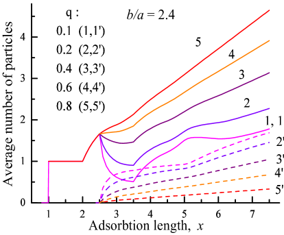
Figure 1: (color online) Average number of adsorbed particles $n_{a}$ (solid lines) and $n_{b}$ (dashed lines) as functions of the length $x$ (measured in units of $a$) of the adsorption interval, assumed initially empty. The results are obtained by iterating Eqs. (1,2) with the assumed ratio of the particle size $b/a=2.4$ and the varying fraction $q$ of $a$-particles in the flux.

Evaluation of $n_{a}(x)$ and $n_{b}(x)$ is readily done by repeated iterations of Eqs. (1,2), going from the small to progressively larger lengths $x$. Results of the numerical recursion are shown in Fig. 1 for a particle size ratio $b/a=2.4$ and varying $q$.

The noteworthy features of the functions $n_{a}(x)$ and $n_{b}(x)$ are (i) the step-like features at $x=a$, $x=b$ (which are replicated with ever smaller amplitudes at $x=na+mb$, where $n$ and $m$ are integers), (ii) the dip in the number of small particles $n_{a}(x)$ at $x=b$, which increases with $p$, and (iii) the reduction of $n_{b}$ with increasing $q$. We also note that for all $q$ the behavior of both $n_{a}(x)$ and $n_{b}(x)$ becomes very close to linear already at $x\approx 7$.

The asymptotic behavior of $n_{a}(x)$ and $n_{b}(x)$ at large $x$ can be obtained by multiplying Eqs. (1,2) by $x-\overline{l}$ and taking the derivative with respect to $x$. The resulting differential equations are satisfied by linear functions of the form

$$n_{a}=\alpha_{a}(x+\overline{l})-q,\ \ n_{b}=\alpha_{b}(x+\overline{l})-p,$$ (9)

where $\alpha_{a}$ and $\alpha_{b}$ are arbitrary constants. When correctly chosen (by matching to the recursive solution) these constants become the partial filling factors. After the matching is done, the total filled length in the asymptotic limit is given by $f(x)=\theta x+(\theta-1)\overline{l},$ where $\theta=a\alpha_{a}+b\alpha_{b}$ is the specific coverage. It is worthwhile to stress that the value of the asymptotic solutions (9) consists precisely in that they are asymptotically exact. Hence they provide a sanity check on any solution we could have obtained by a numerical recursion up to moderate values of $x$.

Similarly, Eqs. (7-9) yield the variances at large $x$,

$$u_{a}-n_{a}^{2} = \mu_{a}(x+\overline{l})-qp[1+(b-a)\alpha_{a}]^{2},$$ (10a)

$$u_{b}-n_{b}^{2} = \mu_{b}(x+\overline{l})-qp[1-(b-a)\alpha_{b}]^{2}.$$ (10b)

Again, these solutions are asymptotically exact; they satisfy Eqs. (7,8) with arbitrary values of $\mu_{a}$ and $\mu_{b}$, provided of course that $n_{a}(x)$ and $n_{b}(x)$ are in the correct asymptotic form (9) with properly chosen [i.e., satisfying Eqs. (1,2)] coefficients $\alpha_{a}$ and $\alpha_{b}$. In principle, we could now follow a procedure similar to above, viz. determine $\mu_{a}$ and $\mu_{b}$ by matching Eqs. (10) against a numerical recursive solution at some moderate value of $x$. However, it would be rather difficult to control the numerical accuracy in this procedure, because of the difference of nonlinear functions that enter Eqs. (10), even though that difference itself behaves linearly with $x$ at large $x$.

Fortunately, our model admits of an exact solution based on the use of Laplace transformation (details can be found in assl and references therein). Below we present an exact evaluation of variance for particles of larger size, while details of similar though lengthier calculations for smaller particles are presented in Appendix.

Firstly, we need exact solutions of Eqs. (1,2). To obtain these, we substitute $x\rightarrow x+b$ in Eq. (2) and multiply it by $x-\overline{l}$. Taking the Laplace transformation of the resulting equation and using the boundary condition (4), we obtain

$$\left[-\frac{d}{ds}+b-\overline{l}\right]e^{bs}N_{b}(s)=\frac{p}{s^{2}}+\frac{2}{s}\left(qe^{(b-a)s}+p\right)N_{b}(s)$$ (11)

Here $N_{b}(s)$ is the Laplace transform of $n_{b}(x)$,

$$N_{b}(s)=\int_{0}^{\infty}e^{-sx}n_{b}(x)dx,$$ (12)

Rearranging the terms and multiplying by $e^{-bs}$, we put Eq. (11) into the form

$$N_{b}^{\prime}(s)+\left[\overline{l}+\frac{1}{s}\left(qe^{-as}+pe^{-bs}\right)\right]N_{b}(s)=-\frac{p}{s^{2}}e^{-bs}.$$ (13)

For $p\rightarrow\infty$, the solution of Eq. (13) is, asymptotically,

$$N_{b}(s)|_{s\rightarrow\infty}=\frac{p}{s(b-\overline{l})}e^{-bs},$$ (14)

as follows from the known variation of $n_{b}(x)\approx p(x-b)/(b-\overline{l})$ at small $x-b$. Hence we have

$$N_{b}(s)=\frac{p\exp(-\overline{l}~{}s)}{s^{2}\beta(s)}\int_{s}^{\infty}e^{-q(b-a)t}\beta(t)dt,$$ (15)

where

$$\beta(s)=\exp\left[-2\int_{0}^{s}\left(\frac{1-q\exp(-at)-p\exp(-bt)}{t}\right)dt\right].$$ (16)

To find the asymptotic behavior of $n_{b}(x)$ at large $x$, it is convenient to use Karamata’s Tauberian theorem for the asymptotic growth rate of steadily growing functions (see e.g. Variat , p. 37). According to the theorem, the asymptotics of $n_{b}(x)$ [or $n_{a}(x)$ or their variances] can be readily obtained (by taking the inverse Laplace transformation) from the Laurent power series expansion of the Laplace transforms of these functions at small $s$ (see coff for the mathematical details of this analysis).

Function $N_{b}(s)$ is analytic at all $s\neq 0$ and at $s=0$ it has a second-order pole with the following asymptotic

$$N_{b}(s)=\frac{\alpha_{b,0}}{s^{2}}+\frac{\alpha_{b,0}\overline{l}-p}{s}+O(s),$$ (17)

where

$$\alpha_{b,0}=p\int_{0}^{\infty}e^{-q(b-a)s}\beta(s)ds.$$ (18)

To calculate $n_{b}(x)$ at large $x$, we take the inverse Laplace transformation of (17). This gives

$$n_{b}(x)=\alpha_{b,0}(x+\overline{l})-p,$$ (19)

with an exponentially small error term, in line with the asymptotics given by Eq. ($\ref{asy_nab})$.

In the limit $p=1$, equation (18) duly gives the so-called jamming filling factor $R$ for the standard RSA, $\alpha_{b,0}(l=1)\equiv R=0.74759\cdots$ (also called the Renyi constant renyi ). In the limit $a\rightarrow 0$, Eq. (18) recovers the results of Refs. bartelt ; hassan1 for the coverage of a line from a binary mixture of finite size particles and point defects. Moreover, Eq. (18) gives the large particle contribution to the total coverage, obtained in mao ; hassan2 for the range $a<b<2a$. Here we see that this result remains valid for arbitrary $a<b$.

Next, we perform similar manipulations with Eq. (8) and obtain an equation for the Laplace transform of the variance $U_{b}(s)=\hat{L}[u_{b}(x)]$, viz.

$$U_{b}^{\prime}(s)+\left[\overline{l}+\frac{2}{s}\left(qe^{-as}+pe^{-bs}\right)\right]U_{b}(s)=-\frac{\exp(-bs)}{s^{2}}R_{b}(s),$$ (20)

where

$$R_{b}(s)=p+4psN_{b}(s)+2s^{2}N_{b}^{2}(s)\left(qe^{(b-a)s}+p\right),$$ (21)

with $N_{b}(s)$ defined by Eq. (15). The solution of Eq. (20) can be written in a form similar to Eq. (15), namely

$$U_{b}(s)=\frac{\exp(-s\overline{l})}{s^{2}\beta(s)}\int_{s}^{\infty}\beta(t)e^{-q(b-a)t}R_{b}(t)dt.$$ (22)

The integrand in the right-hand side of Eq. (22) is proportional to $1/t^{2}$ causing the integral to diverge as $1/s$ for $s\rightarrow 0$. This is due to the square-law dependence of $u(x)$ at large $x$ .

To separate the regular part needed for the estimation of variance, we note that at small $t$ one has $R_{b}(t)\propto\alpha_{b,0}t^{-2}$. Moreover, the series expansion shows that the difference $\beta(t)\exp[-q(b-a)t]R_{b}(t)-2\alpha_{b,0}^{2}t^{-2}$ is regular at $t\rightarrow 0$. Therefore, it is convenient to define an entire function $\kappa_{b}(t)=\beta(t)\exp[-q(b-a)t]R_{b}(t)-2\alpha_{b,0}^{2}t^{-2}$. In terms of this function, the solution $U_{b}(s)$ can be expressed as follows:

$$U_{b}(s)=\frac{\exp(-s\overline{l})}{s^{2}\beta(s)}\left[\frac{2\alpha^{2}_{f,0}}{s}+k_{b,0}-\int_{0}^{s}\kappa_{b}(t)dt\right],$$ (23)

where

$$\ \ k_{b,0}=\int_{0}^{\infty}\kappa_{b}(t)dt.$$ (24)

To apply Karamata’s Tauberian theorem, we note that the asymptotic expansion of $U_{b}(s)$ near its third-order pole is of the form

$$U_{b}(s) = \frac{2\alpha_{b,0}^{2}}{s^{3}}+\frac{k_{b,0}+2\alpha_{b,0}^{2}\overline{l}}{s^{2}}$$ (25)

$$+\frac{k_{b,0}\overline{l}-\kappa_{b}(0)-qp(b-a)^{2}\alpha_{b,0}^{2}}{s}.$$

Taking the inverse Laplace transformation, we find the asymptotic form of $u_{b}(x)$:

$$u_{b}(x) = \alpha_{b,0}^{2}x^{2}+(k_{b,0}+2\alpha_{b,0}^{2}\overline{l})x$$ (26)

$$+k_{b,0}\overline{l}-\kappa_{b}(0)-qp(b-a)^{2}\alpha_{b,0}^{2},$$

with an exponentially small error term. Using Eq. (19) to subtract $n_{b}^{2}(x)$, we find an equation of the form (10b) with $\mu_{b}=k_{b,0}+2p\alpha_{b,0}$. The specific variance of the adsorbed number of $b$-particles is given by (at $x\rightarrow\infty$)

$$\mu_{b} = \alpha_{b,0}(1+2p)+2\int_{0}^{\infty}\left\{\beta(s)sN_{b}(s)e^{\overline{l}s}\left[2pe^{-bs}\right.\right.$$ (27)

$$\left.\left.+sN_{b}(s)\left(qe^{-as}+pe^{-bs}\right)\right]-\frac{\alpha_{b,0}^{2}}{s^{2}}\right\}ds.$$

Integrating by parts the last term and rearranging the result, we finally obtain

$$\mu_{b} =\alpha_{b,0}(1-2p)+4p\int_{0}^{\infty}\frac{\alpha_{b}(u)}{u}e^{-bu}\left(1-qe^{-au}\right.$$ (28)

$$\left.-pe^{-bu}\right)du+2\int_{0}^{\infty}\frac{\alpha^{2}_{b}(u)}{\beta(u)u^{2}}e^{-\overline{l}u}K(u)du,$$

where

$$K(u) =qe^{-au}\left[2(1-qe^{-au}-pe^{-bu})-(a+\overline{l})u\right]$$ (29)

$$+pe^{-bu}\left[2(1-qe^{-au}-pe^{-bu})-(b+\overline{l})u\right]$$

and

$$\alpha_{b}(u)=\alpha_{b,0}-p\int_{0}^{u}e^{-q(b-a)y}\beta(y)dy.$$ (30)

In the limit of small $p\rightarrow 0$, the Fano factor $\Phi=\mu_{b}/\alpha_{b,0}\rightarrow 1$. In this limit, large particles are distributed on the line randomly, without correlations. In the opposite limit, $p=1$, Eq. (28) reduces to the standard RSA result, first obtained for a lattice RSA model by Mackenzie Mack . The numerical value of the Mackenzie constant, $\mu_{0}=0.0381564\cdots$, corresponds to $\Phi=0.0510387\cdots$, see coff . Expression (28) for the larger particles has the same structure as the corresponding formula in the standard RSA model (fixed-size CPP). Due to the exponential factors in the integrands of Eq. (28), the dependence of $\mu_{b}$ on $a$ for $a\ll b$ is quite weak. The limiting value of the specific variance for $a/b\rightarrow 0$ gives the specific variance of the fill factor for the case of finite-size particles ($b=1$) mixed with point-size particles,

$$\mu_{b,p} =\alpha_{b,p,0}(1-2p)+4p^{2}\int_{0}^{\infty}\frac{\alpha_{b,p}(u)}{u}e^{-u}\left(1-e^{-u}\right)du$$ (31)

$$+2p\int_{0}^{\infty}\frac{\alpha^{2}_{b,p}(u)}{\beta_{p}(u)u^{2}}\left\{qe^{-pu}\left(2-2e^{-u}-u\right)\right.$$

$$\left.+e^{-(1+p)u}\left[2p\left(1-e^{-u}\right)-(1+p)u\right]\right\}du,$$

where $\alpha_{b,p,0}$ is the fill factor for this case,

$$\alpha_{b,p}(u)=p\int_{u}^{\infty}e^{-qy}\beta_{p}(y)dy,\ \ \alpha_{b,p,0}=\alpha_{b,p}(u=0)$$ (32)

and

$$\beta_{p}(u)=\exp\left[-2p\int_{0}^{u}\left(\frac{1-\exp(-t)}{t}\right)dt\right].$$ (33)

It is worth to note that Eqs. (2,8) and their solutions can be readily generalized to the case when particles of the smaller size have an arbitrary distribution in the interval $[a_{1},a_{2}]$ so long as $a_{2}\leq b$ asslr .

The above analytic results for the variance of larger particles are essentially exact, as will be confirmed in the next Section by Monte Carlo simulations. For the smaller particles, the calculations are messier and accurate analytical results can be obtained only in a certain range of particle size ratios. Estimations of the variance for small-size particles are further discussed in the Appendix.

III Discussion of the results, comparison with Monte Carlo modeling

Here we present the results of numerical calculations using both the analytical expressions obtained in the preceding section and Monte Carlo simulations. For large-size particles the Monte Carlo results are very close to analytical expressions both for the fill factor and the variance, so we shall not dwell on their comparison. For small-size particles, especially in the range $2<b/a<8$, analytical calculations are rather unwieldy, so Monte Carlo simulations become indispensable. Larger size ratios, $b/a>8$, lend themselves to an approximate analytical approach (see Appendix). In this case, we use the Monte Carlo to estimate its accuracy for the small particle contribution.

Traditional studies of the generalized RSA via Monte Carlo simulations follow a temporal sequence of events. For the case of adsorption on a line of the length $x$ from a binary mixture, one step of the sequence comprises:

(i) selection of a particle from the mixture according to the deposition flux ratio (with the probability $q$ of choosing the small-size ($a$) particle, and the probability $p=1-q$ of selecting a particle of larger size $b$);

(ii) random choice of a deposition coordinate of particle center on the line $x$ with formerly deposited particles;

(iii) rejection of the particle if it overlaps by any part with formerly deposited particles or with the line borders; otherwise, the particle deposition proceeds with the formation of two new disconnected adsorption lengths.

This traditional approach has several drawbacks, that make the modeling very demanding, both in terms of the computer time and memory allocation.

Firstly, both the filled length in the jamming limit and the specific fill factor (coverage) depend on the initial length. Due to the self-averaging property of the coverage it tends to a unique exact value in the limit $x\rightarrow\infty$. To obtain the accuracy of about $0.1$ %, the common strategy has been to use large initial length values (10${}^{5}b$ -$10^{7}b$) and make additional averaging over a set of about $N_{R}=$100-1000 different realizations.

Secondly, as time evolves and the jamming limit is approached, the probability of finding a free gap for particle deposition becomes greatly reduced, so that the adsorption time tends to infinity. The process is terminated when variations of the adsorbed particle number are smaller than those required by the desired accuracy.

The recursive analysis of the generalized RSA suggests a revision of the above scheme. Since the deposition is random and sequential, it does not depend on the temporal history of the process or the growing number of rejected particles and their coordinates. Therefore one step of the sequence can be chosen as follows:

(i) selection of any free deposition length, $l_{1}>a$. It is convenient to choose for $l_{1}$ the outermost free deposition length on the left-hand side.

(ii) if $l_{1}<b$, then particle of size $a$ is deposited, otherwise the deposited particle is chosen according to the landing probability, given by $q(l_{1}-a)/(l_{1}-\overline{l})$ for $a$-particle and $p(l_{1}-b)/(l_{1}-\overline{l})$ for $b$-particle, where $\overline{l}=qa+pb$.

(iii) random choice of a deposition coordinate (taken as the coordinate of particle’s left end) on the line $l_{1}$ for a given particle size, i.e. within the interval $l_{1}-a$ for $a$-size or within $l_{1}-b$ for $b$-size particle, with the formation of two new adsorption lengths from the initial length $l_{1}$.

It is readily seen that although the sequence of deposition events is different from the actual temporal sequence of adsorption (the simulated deposition proceeds by sequentially filling the left-hand lengths), the statistics of divisions is identical and therefore so is the final distribution of the gaps, as well as all statistical properties of the jamming state. Our sequential scheme excludes deposition of to-be-rejected particles and therefore is incomparably faster. Besides, it terminates exactly when the jamming limit (with no gaps larger than unity) is achieved. Direct comparison with the traditional Monte Carlo results, e.g. hassan1 ; Araujo ; mao exhibits total agreement. The difference in the calculation time is especially evident for small (close to zero) $q$: in the time scale of “real” deposition, the jamming limit will be strongly delayed because of the rarity of events with small particle chosen. In our modified approach, all gaps smaller than $b$ are “rapidly” populated by small-size particles, however small be the value of $q$.

The next step of the revision is to exploit the fact (proven analytically in the preceding section) that in the jamming limit, the linear dependence on the adsorption length of both the average filled length and its variance is exponentially accurate, starting from a reasonably short length, certainly not exceeding $x\approx 10b$. Since this linear dependence has only two parameters [actually only one, as the parameter ratio is exactly fixed by analytical considerations, Eqs. (9,10)], both the coverage and the variance can be determined with Monte Carlo simulations of short samples.

To be sure, in order to achieve the same accuracy as that obtained for long samples, the results should be averaged over a sufficient number of realizations $N_{R}$. This, however, takes little memory or time. Calculations show similar accuracy for different $x$ and $N_{R}$, so long as their product $x\times N_{R}$ is fixed. The results presented below were obtained using a sample of size $x=200a$ for $b/a<10$ and $x=400a$ for $b/a=20,40$, subsequently averaged over 10 000 realizations, which appeared to be sufficient to eliminate any spread of the results in the graphical presentation (producing an accuracy of better than 0.1%).

The use of small samples is very effective in reducing the calculation time (with an ordinary PC, high-accuracy results can be obtained in minutes, compared to days in the traditional scheme mao ).

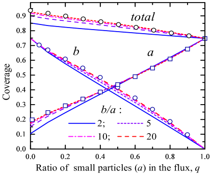
Figure 2: (color online) Partial contributions of small and large particles to the total coverage depicted as functions of $q$, for different particle-size ratios $b/a$ in the flow. Open points correspond to the limit $b/a\gg 1$, as described by the analytical formulae (32) for $b$-particles and (47) for $a$-particles. For the total coverage, the open circles to the wasted length product approximation, Eq. (34).

Figure 2 shows partial contributions to the coverage as functions of the fraction $q$ of small particles in the binary mixture at different ratios of particle size. As $q$ increases, the coverage with large particles is substituted by that with small particles, producing some decrease in the total coverage. In the regions of corresponding parameters, our results reproduce those of reported analytical calculations (i.e. for $b/a<2$ hassan1 ; mao and for $a=0$ hassan2 for the large particle contribution) and those obtained by the Monte Carlo simulations of hassan1 ; Araujo ; mao , demonstrating the validity of our revised approach.

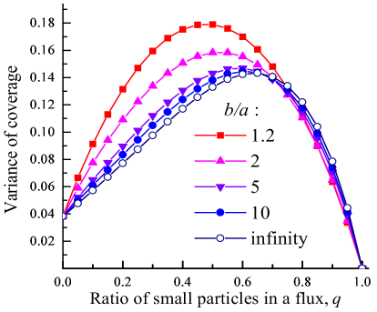
Figure 3: (color online) Variance of the partial coverage by adsorbed $b$-particles from the binary mixture for different values of the particle size ratio $b/a$ in the flow.

It is evident from Fig. 2, that the total coverage increases at smaller $q$, as can be explained by sequential deposition of the two kinds of particles. In the regime of small $q$, large particles are adsorbed first and their deposition, unobstructed by small particles, is tight. Subsequently, the small particle fill the gaps between large particles and this clearly reduces the total wasted length.

The effect of increasing the particle size ratio $b/a$ is pronounced only for $b/a<10$, then it rapidly saturates. Therefore, for large $b/a$, say $b/a=20$ the coverage by large particles is very close to that obtained for a model mixture of point-like and finite-size particles [by formally letting $a=0$ in Eq. (18)]. Such a model, however, has little relevance to any practical situation, because it simply ignores the partial contribution of small particles to the total coverage. The latter can be described analytically in the limiting case $b/a\rightarrow\infty$, Eq. (47).

The partial contribution of small particles steadily grows with the increasing size ratio due to the expanding gaps between the large particles. In the limit $q\rightarrow 0$, the total coverage can be estimated by observing that the specific wasted length in this case is a simple product of the specific lengths wasted in initial deposition of large particles and subsequent deposition of small particles, i.e. $1-\theta=(1-\theta_{a})(1-\theta_{b})$. Since for $q=0$ the specific coverage $\theta_{b}=R$ and since for large size ratios (when the gaps between large particles are large) the specific coverage $\theta_{a}=R$, we have $\theta=1-(1-R)^{2}$=0.936, in agreement with the results reported in the literature hassan1 ; Araujo . However, the sequential nature of the deposition suggests that the entire $q$ dependence of the total $\theta$ can also be approximated by a product of the specific wasted lengths in the competitive deposition of large particles $q(1-R)$ and subsequent deposition of small particles in the remaining gaps, which gives

$$\theta=1-(1-R)(1-pR)=R[1+p(1-R)].$$ (34)

This product-waste approximation is shown in Fig. 2 by the open circles.

Next, we concentrate on the specific waste variance and the Fano factor. We shall discuss the $b$- and $a$-particles separately, since the effects are rather different in nature and also since they have been evaluated by different techniques. Results for large particles are obtained by numerical integration of Eq. (30) and confirmed by Monte Carlo simulations. Results for $a$ particles are obtained by Monte Carlo stimulations and are accompanied by analytical expressions in the limit $b/a\gg 1$.

Variance, $\tilde{\mu}$, of the partial contribution of $b$-particles to the total coverage is shown in Fig. 3 for different particle size ratios. Unlike the particle number variance $\mu$, the variance of coverage, $\tilde{\mu}=\mu b$, depends only on the size ratio $b/a$ and does not directly scale with $b$. It is therefore more indicative of the effect of decreasing size of small particles on the fluctuations of the number of large particles. At $q\rightarrow 0$, when the adsorption of large particles is unconstrained by small particles, the variance of large particles is minimal and corresponds to the highly correlated distribution corr in the standard CPP problem (one-size RSA). The variance rapidly increases with $q$ as the small particle deposition destroys the CPP correlations. The maximum of this effect is shifted to larger $q$ values for larger $b/a$. For $q$ approaching unity, the variance decreases simply due to the decrease of the average number of adsorbed $b$-particles.

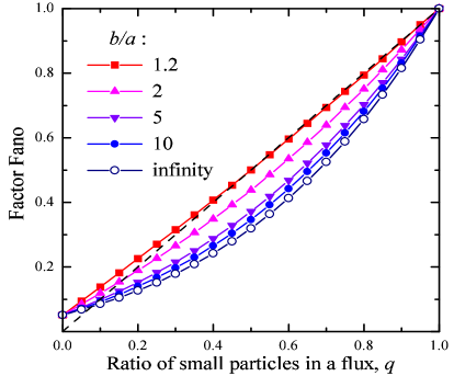
Figure 4: (color online) The Fano factor for the number of adsorbed $b$-particles from the binary mixture as functions of $q$, for different values of the ratio $b/a$ of particle sizes in the flow. Dotted line corresponds to a random particle packing on a lattice with suitable lattice constant (aka monomer adsorption).

Correlation effects are more adequately characterized by the Fano factor $\Phi_{b}$, shown in Fig. 4. With the increasing number of competing small particles in the flux, the Fano factor grows from the smallest value $\Phi=0.051\cdots$, corresponding to the one-size RSA problem, to unity in the limit $q\rightarrow 1$. Small coverage by the large particles in the latter limit means that they are distributed randomly on the line, so that Poisson statistics recovers. The most noticeable effect is a rapid decrease of the Fano factor with $1-q$, manifesting a strong enhancement of the correlation effects in the large particle distribution. These correlation effects become exhausted only near $q\leq 0.1$. The correlation effects increase with $b/a$ but saturate at about $b/a=20$.

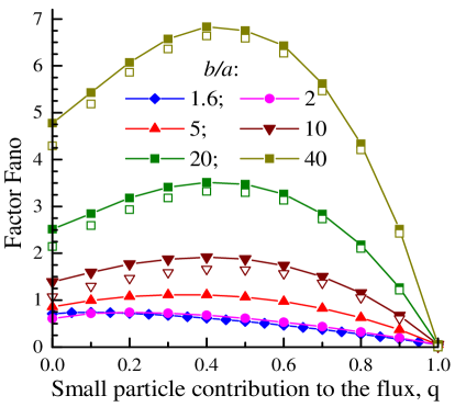
Figure 5: (color online) The Fano factor for adsorbed $a$-particles from the binary mixture for different values of the particle size ratio $b/a$ in the flow. Open points show the contribution of fluctuations of the gap sizes between large particles.

Figure 5 shows the Fano factor for $a$-particles competitively deposited along with large particles. The results are strikingly different at all $q\neq 1$ (when $\Phi_{a}=\Phi$, as expected). While the distribution remains correlated ($\Phi_{a}\leq 1$) for small ratios $b/a\leq 5$, at larger $b/a$ one has $\Phi_{a}>1$, almost for all $q$, which means that the number of small particles per unit length is strongly fluctuating. This is due to the widely fluctuating size of the gaps available for small particle deposition between large particles. For large values of $b/a$ and in the entire range of $q$, the Fano factor $\Phi_{a}$ can be approximated in terms of the fluctuations of the coverage by the large particles, viz. $\Phi_{a}=(b/a)\mu_{b,p}R^{2}/\theta_{a}$, where $\mu_{b,p}$ is given by Eq. (31) and $\theta_{a}$ by Eq. (47). This approximation, which neglects fluctuations of the density of adsorbed $a$ particles in the gaps, is shown in Fig. 5 by open points. This contribution is proportional to $b/a$ and for $b/a>10$ it is evidently dominant.

For the particle energy branching process at small $b/a<2$, both the variance of the partial numbers of small and large particles and the total number variance are of importance. We shall illustrate this point in the instance of $b/a=1.2$ shown in Fig. 6. We see that at $q\approx 0.5$ the fill factor fluctuations are larger for $a$ particles and somewhat smaller for $b$ particles, but both are pretty large, compared to the variance of the total number of adsorbed particles. This is due to the strong anti-correlation in their distribution, as evidenced by the specific fluctuation correlation function, $f_{cor}=x^{-1}\langle\delta n_{a}\delta n_{b}\rangle$, also plotted in Fig. 6. We note that $f_{cor}<0$, which means that any excess in the number of $a$-particles is accompanied by a downward fluctuation in the number of adsorbed $b$-particles. Importantly, the variance and the Fano factor for the total number of adsorbed particles does not exceed substantially its value for the single-size RSA.

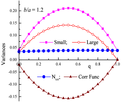
Figure 6: (color online) Variance of the partial number of adsorbed $a$- and $b$-particles and of the total number of adsorbed particles for $b/a=1.2$. Also shown is the fluctuation correlation function $f_{cor}$.

Note the asymmetry of the curves for $a$ and $b$ particles, e.g. the variance of large particles goes to zero as $q\rightarrow 1$ whereas that of small particles remains finite even as $q\rightarrow 0$. This is a feature of our model that allows ”infinite” amount of time for the deposition of small particles in the gaps left after the deposition of large particles is completed, but not vice versa. Therefore, the deposition of small particles remains finite even in the limit of $q\rightarrow 0$ and the same is true for the $a$-particle number variance.

Another interesting feature of the $a$-particle number variance, already evident from Fig. 5, is its non-monotonic behavior as function of $b/a$ at small $q$. This variation is displayed directly in Fig. 7 that shows the dependence of the Fano factor on $b/a$ for $q$=0.05, 0.1 and 0.2 — where its non-monotonic nature is most pronounced. The minimum of the Fano factor is achieved at $b/a\approx 2$. Note that the non-monotonic dependence of the Fano factor is accompanied by non-monotonic variations in the dispersion of the gaps between small particles. In Ref. Araujo it was found that for $q=$0.5 the dispersion is noticeably reduced at $b/a\approx 1.55$. These effects were interpreted as a manifestation of the so-called “snug fit” events, i.e. particle deposition in gaps that are just barely above the unit length $a$. In contrast, the Fano factor for $b$-particles and that for the total number of particles remain monotonic everywhere.

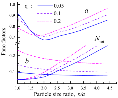
Figure 7: (color online) The Fano factor for adsorbed $a$- and $b$-particles as functions of the particle size ratio $b/a$. Also shown is the Fano factor for the total number of adsorbed particles.

IV Some consequences for the energy branching in high-energy particle detectors

The model of RSA from binary mixtures is relevant to an important practical problem of particle energy branching (PEB) where high-energy particle propagates in an absorbing medium and multiplies producing secondary electron-hole (e-h) pairs. Multiplication proceeds so long as the particle energy is above the impact ionization threshold Spieler . The energy distribution of secondary particles is random to a good approximation.

The affinity between the two problems was fully recognized already in 1965 by van Roosbroek rusb (see also Alkhas ). The PEB process can be considered in terms of a CPP if one identifies the initial particle kinetic energy with an available parking length and the pair creation energy with the car size. Similarly, the kinetic energies of secondary particles can be identified with the new gaps created after deposition of a particle. Full equivalence of PEB to CPP further requires that only one of the secondary particles takes on a significant energy, which corresponds to binary cascades Nay . Otherwise, one has to consider a simultaneous random parking of two cars in one event.

To estimate the particle initial energy in PEB, one measures the number $N$ of created electron-hole pairs. Variance of this number, due to the random character of energy branching and also due to random energy losses in phonon emission, limits the accuracy of energy measurements. Both the yield $\overline{N}$ and the e-h pair variance ${\rm var}(N)=\overline{(N-\overline{N})^{2}}$ are proportional to the initial energy. The ratio of the e-h pair variance to the yield, i.e. the Fano factor of the PEB process, is a parameter that quantifies the energy resolution of high-energy particle detectors.

For semiconductor crystals, the PEB problem has additional complications due to the energy dependence of phonon losses and the energy dependence of the electron density of states and the impact ionization matrix element. Full quantitative analysis of the PEB is possible only with detailed numerical calculations, which goes far beyond the scope of the present article.

A common feature of the energy branching process in semiconductors is the presence of several pair production channels, associated with the multi-valley energy band structure of the crystal. In Si, Ge and common A₃B₅ semiconductors, the e-h pair creation produces electrons in one of the ellipsoids near the edge of the Brillouin zone, in 100 (X) or 111 (L) directions. Owing to the difference in the final densities of states and the matrix elements, the impact ionization processes associated with X and L valleys have different but competitive probabilities. Because of its low density of states, the $\Gamma$ valley is usually not competitive, even when it is the lowest valley.

Ultimately, electrons will end up in the lowest energy valley but when the final electron valley is itself degenerate, as in Ge or Si, the resulting electron states may not be fully equivalent, because of the different collection kinetics owing to the crystal anisotropy. This effect may have important consequences for the observed variance. For example, in Si diode detectors electrons are created in 6 degenerate energy valleys that represent ellipsoids of revolution elongated along (100) and equivalent directions in k-space. Suppose the diode structure is such that the current flows along the (100) direction, as it is usually the case. Electrons from the two valleys along the current have a large mass and low mobility. The measured current is hence dominated by electrons from the 4 valleys elongated perpendicular to the current that have a low mass and high mobility along the current. Since the choice of equivalent valley in the PEB process is fully random, the number of high-mobility electrons will fluctuate more strongly than the total number of generated carriers. These fluctuations will dominate if the inter-valley transition rate is low compared to the inverse collection time. In the opposite limit of high inter-valley transition rates, this effect will average out as the collected current will fluctuate in time. The current fluctuation mechanism due to the carrier escape into heavy-mass valleys is a well-known source of noise in multi-valley semiconductors Kogan ). More detailed account for these effects will be presented elsewhere asslr .

Here we shall discuss an opposite situation, that is common to direct-gap semiconductors, such as GaAs or InP. In these materials, the lowest ($\Gamma$) electron valley has a very low density of states, compared to that in the satellite (X and L) valleys. Therefore, the probability of electron generation in the $\Gamma$-valley can be neglected in first approximation, so that the branching competition occurs only between the satellite valleys of two different kinds. Both the density of states and the threshold energy are different between X and L valleys and we can use the results of the present study to interpret and predict the consequences, at least qualitatively.

The binary-mixture RSA model interprets the higher density of states as higher deposition rate and the higher threshold as larger particle size. To make our conclusions more transparent, let us re-formulate the required results in terms of a random parking problem with cars of two sizes. We are now interested only in the numbers of parked cars and the fluctuations of these numbers.

Several qualitative conclusions can be drawn from our results:

(i) The total number of parked cars (in the jamming state) will decrease with increasing fraction of larger cars in the flow and with the growth of their size. For $b/a=1.4$ the effect is illustrated in Fig. 8 (which can be viewed as an extension of Fig. 2). It follows from the fact that adsorption of a large car excludes larger length for subsequent parking events and thus causes a decrease of the total fill factor. Note that the decrease in the total particle number is accompanied by an increase in the total filled length, as smaller number of cars cover larger area.

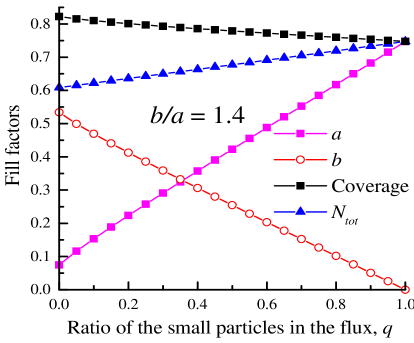
Figure 8: (color online) Partial fill factors and the total coverage for $b/a=1.4$ as a function of $q$. Also shown is the total number $N_{tot}$ of adsorbed particles

The next two conclusions (ii) and (iii), illustrated in Fig. 6, are interconnected and will be discussed jointly.

(ii) Variance of the total number of parked cars and the Fano factor will both grow with the increasing fraction of larger cars in the flow and with the growth of their size.

(iii) Variance of the separate numbers of parked small and large cars and their Fano factors are considerably larger than that of the total number of cars. Therefore, if for some reason one type of cars is neglected or undercounted, the registered variance and the Fano factor can be substantially increased.

These conclusions are connected with the nature of the car number fluctuations and the strong anti-correlation between the fluctuations in the number of small and large cars. Fluctuations in the number of parked cars of one kind are strongly enhanced by the presence of more or less randomly distributed cars of the second kind, especially when cars of the second kind dominate. This leads to conclusion (iii). However, the two distributions are anti-correlated (higher number of parked small cars is accompanied by a smaller number of large cars and vice versa). The anti-correlation is particularly strong for a size ratio that is close to unity.

One can imagine a case when the two kinds of cars differ only in “color”. In this case, Eqs. (18,28) yield $\alpha_{a,0}=qR$, $\alpha_{b,0}=pR$, $\mu_{a}=Rqp+q^{2}\mu_{0}$ and $\mu_{b}=Rqp+p^{2}\mu_{0}$, so that at large $x$ we have $<\delta n_{a}\delta n_{b}>/x=-(R-\mu_{0})qp$. Then, the anti-correlation is almost complete: the fluctuations of the total number are much smaller than those of a given color, but still non-zero. Both the individual-color number fluctuations and the anti-correlation are largest at $q\approx 0.5$, cf. Fig. 6. The anti-correlation decreases with increasing size ratio, as reflected in our conclusion (ii).

To discuss the above conclusions in terms of the PEB problem, we note that estimation of the initial particle energy is equivalent in CPP to a measurement of the unknown length of a parking lot in terms of the total number of cars that were able to fit into it by random parking, assuming that the average fill factor for a given two-size car mixture is known from earlier measurements. The absolute accuracy of such a measurement depends on the variance of the fill factor, and the relative accuracy is determined by the Fano factor. As shown above for a mixture of cars, the larger disparity of car sizes leads to the higher fill-factor variance and therefore reduces the absolute accuracy.

A particle detector measures the total number of secondary particles of all sorts (but not their total creation energy, that would be equivalent to the filled length). In any channel, all secondaries that have sufficient energy for further branching will do so. Therefore, only those pair creation energy ratios that leave the channels competitive (i.e. $b/a<2$) are relevant to the PEB problem — otherwise additional energy branching would be possible.

We conclude that the presence of competing channels with different energies [e.g. impact ionization with excitation in X and L valleys] will decrease the quantum yield (the number of secondaries per unit energy of the primary particle) and enlarge the Fano factor. The attendant loss in energy resolution is not that bad when the ionization energies associated with different valleys are not too disparate. For example, in Ge besides the lowest eight L valleys ($E_{G}=0.66\>$eV) one has a non-competitive $\Gamma$ valley ($E_{\Gamma}=0.8\>$eV) and six very competitive Si-like valleys ($E_{G}=0.85\>$eV). The downgrading of energy resolution should be more important for crystals with larger ($\approx 2$) threshold energy ratio. For example, in Si one has besides the 6 lowest valleys ($E_{G}=1.12\>$eV) in X direction, eight germanium-like L valleys with the gap $E_{L}=2.0\>$eV. Their effect on the Fano factor in silicon may not be negligible.

Finally, reformulating (iii), we stress that any significant disparity in the collection efficiency between different equivalent valleys will strongly enhance the Fano factor and downgrade energy resolution. This happens because any collection disparity breaks the symmetry between the equivalent valleys and destroys the anti-correlation, responsible for keeping the total Fano factor low even when the partial particle numbers associated with individual valleys exhibit fully random fluctuations. One possible origin for the asymmetry in the collection efficiency in semiconductors has been discussed above in the case of silicon diodes with the electric field in (100) direction. In germanium diodes all different valleys are equivalent relative to the (100) direction and the symmetry is not broken. It would be broken, however, if one were to use Ge diodes oriented in (111) direction. This would lead to a situation similar to Si — with a possible degradation in the Fano factor. These effects deserve additional study, both experimental and theoretical.

V conclusions

We have studied a generalized 1-dimensional competitive random sequential adsorption problem from a binary mixture of particles with varying size ratio. Using a recursive approach, we obtained independent equations for the number of adsorbed particles of given sort and exact analytical expressions for the partial filling factors and variances for the larger particles. For the smaller particles analytical expressions were obtained in a number of limiting cases. The results have been confirmed by direct Monte Carlo simulations. To do so, we have introduced a modified Monte Carlo procedure that enabled us to explore a wide range of particle size ratios and particle fractions in the flux.

A number of qualitative implications have been formulated, relevant to the energy branching problem in high-energy particle propagation through a semiconductor crystal. Conclusions made concern the quantum yield and the energy resolution in semiconductor detectors made of crystals with several competing channels of impact ionization with different final electronic states.

We have found a very strong anti-correlation effects which strongly suppress fluctuations of the total particle number compared to the fluctuations of partial contributions by particles of a given sort. This effect is particularly evident when one considers the deposition of similar competing particles, e.g. parking of cars that are different only in “color”. It may have dramatic consequences for semiconductor $\gamma$-radiation detectors, if the symmetry between anti-correlated particles is broken by a biased collection. This leads to an important conclusion that the energy resolution of semiconductor detectors is very sensitive to the collection efficiency of competing secondary particles.

We have also found a very strong correlation effects that suppress fluctuations of the larger particle number for all particle ratios. As a result, the Fano factor for the larger particles is as a rule considerably smaller than that for the smaller particles. The variance of the coverage by the smaller particles strongly increases with the growth of the particle size ratio $b/a$. This effect is due to the fluctuations in the size of gaps between larger particles that serve as receptacles for small-particle deposition. For $b/a\geq 5$ the small-particle variance exceeds that for the Poisson distribution in almost the entire range of particle fractions in the flux onto the adsorbing line.

Acknowledgement. This work was supported by the New York State Office of Science, Technology and Academic Research (NYSTAR) through the Center for Advanced Sensor Technology (Sensor CAT) at Stony Brook.

Appendix A Small particle contributions to coverage and coverage variance

To calculate the contribution of small particles to the total coverage at large $x$, we use Eq. (1) with the initial boundary conditions (5). With the substitution $x\rightarrow x+b$ and using Eq. (6), we rewrite Eq. (1) in the form

$$(x+b-\overline{l})n_{a}(x+b)=q(b-a)n_{a}(b)+qx$$

$$+2q\int_{b-a}^{x+b-a}n_{a}(y)dy+2p\int_{0}^{x}n_{a}(y)dy$$ (35)

Equation (35) is valid for all $x\geq b$. Taking Laplace transformation of $n_{a}(x)$ cut at $x<b$ by a step-function factor, we find that the transform,

$$\tilde{N}_{a}(s)=\int_{b}^{\infty}e^{-sx}n_{a}(x)dx,$$ (36)

satisfies the following equation

$$\left(-\frac{d}{ds}+b-\overline{l}\right)e^{bs}\tilde{N}_{a}(s)=\frac{q}{s^{2}}[1+(b-a)n_{a}(b)s]$$

$$+2\frac{q}{s}e^{(b-a)s}\left[\tilde{N}_{a}(s)+J_{1}(s)\right]+2\frac{p}{s}\left[\tilde{N}_{a}(s)+J_{2}(s)\right]$$ (37)

Here

$$J_{1}(s)=\int_{b-a}^{b}e^{-sx}n_{a}(x)dx,\ \ J_{2}(s)=\int_{0}^{b}e^{-sx}n_{a}(x)dx$$ (38)

Rearranging the terms, we rewrite it in form

$$\left[\frac{d}{ds}+\overline{l}+\frac{2}{s}\left(qe^{-as}+pe^{-bs}\right)\right]\tilde{N}_{a}(s)=-\frac{1}{s^{2}}e^{-bs}R_{a}(s)$$ (39)

where

$$R_{a}(s)=q[1+(b-a)n_{a}(b)s]+2s\left[qe^{(b-a)s}J_{1}(s)+pJ_{2}(s)\right]$$ (40)

The form of Eq. (39) is similar to Eq. (20) in which, however $R_{a}$ should be calculated through $J_{1}(s)$ and $J_{2}(s)$, using Eqs. (5,6). For the case $b<2a$ we have $n_{a}(b)=1$, and $J_{1}(s)=J_{2}(s)$, while the explicit expression for $J_{1}(s)$ is easily obtained by substituting $n_{a}(x)=1$ in Eq. (38). Solution of Eq. (39) then enables one to retrieve the result of Ref hassan1 . To calculate $J_{1}(s)$ and $J_{2}(s)$ for $b>2a$, it is necessary to use Eq. (6), which describes RSA of small particles onto a short line $x<b$. Its analytical solution and therefore the explicit expressions for $J_{1}(s)$ and $J_{2}(s)$ can be obtained for the case $b/a<5$ using direct recursion to find $n_{a}(x)$ (for one-particle RSA problem!). The result is rather cumbersome but suitable for numerical integration.

For the case $b/a>5$ one can exploit the exponentially rapid approach of the solution of Eq. (6) to its asymptotic behavior in the limit $x\gg 1$ (see e.g. Lal for the numerical data). This asymptotic solution,

$$n_{a}(x)=\frac{R}{a}(x+1)-1,$$ (41)

can be used to calculate $J_{1}(s)$ and then $J_{2}(s)$. To do this, we multiply Eq. (6) by $\exp(-sx)$ and integrate between 0 and $b-1$. We obtain an equation for $J_{2}(s)$ of the form

$$J_{2}^{\prime}(s)+\left(a+\frac{2}{s}e^{-as}\right)J_{2}(s)=-\frac{1}{s^{2}}\left\{e^{-as}I(s)\right.$$

$$\left.+s(b-a)e^{-bs}[n_{a}(b)-1]+2se^{-as}J_{1}(s)\right\},$$ (42)

where

$$I(s)=\int_{0}^{(b-a)s}dyye^{-y}.$$ (43)

Solution of Eq. (42), satisfying the boundary conditions for $n_{a}$ given by Eq. (5), is of the form

$$J_{2}(s) = \frac{1}{\tilde{\beta}(s)s^{2}}e^{-as}\int_{0}^{s}dt\tilde{\beta}(t)\left[n_{a}(b)(b-a)te^{-(b-a)t}\right.$$ (44)

$$\left.+2tJ_{1}(t)-\left(1-e^{-(b-a)t}\right)\right]$$

with

$$\tilde{\beta}(t)=\exp\left[-2\int_{0}^{at}\left(\frac{1-e^{v}}{v}dv\right)\right].$$ (45)

The contribution of small particles to the fill factor is then given by

$$\alpha_{a}=\int_{0}^{\infty}\beta(u)R_{a}(u)du.$$ (46)

in which $\beta(u)$ is given by the Eq. (16) and $R_{a}(u)$ is defined by Eq. (40). The obtained solution, though rather unwieldy, is suitable for numerical integration and for $b/a>5$ it gives the results that agree with Monte Carlo simulations.

In the limiting case $b/a=b/a\gg 1$ it reduces to a more compact final expression for the contribution to the total coverage from the small particles

$$\theta_{a}=R\left\{1+\int_{0}^{\infty}due^{-qu}\beta_{p}(u)\left[q(u-1)-2pe^{-u}\right]\right\},$$ (47)

with $\beta_{p}(u)$ defined by (33). For $q=1$, Eq. (47) properly gives $\theta_{a}=R$, while for $q=0$ one has $\theta_{a}=R(1-R)$. The latter expression corresponds to the coverage by small particles of the gaps between the large particles left after their initial deposition. For arbitrary $q$, the coverage given by Eq. (47) is depicted in Fig. 2 by the open squares.

Similar approach can be used to calculate the small particle coverage variance. However, for $b/a>2$ the equation for the Laplace transform of $u_{a}(x)$ given by Eq. (7), including all contributions to $N_{a}(s)$, becomes rather impractical. In the limiting case $b/a\gg 1$, when fluctuations of the large particle gaps dominate the variance of small-particle coverage, one gets a more compact result shown in Fig. 5.

References

- (1) G. J. Rodgers and Z. Tavassoli, Phys. Lett. A 246, 252 (1998).
- (2) D. Boyer, J. Talbot, G. Tarjus, P. Van Tassel, and P. Viot, Phys. Rev. E 49, 5525 (1994).
- (3) A. V. Subashiev and S. Luryi, Phys. Rev. E 75, 011123 (2007).
- (4) M. C. Bartelt and V. Privman, Phys. Rev. A 44, R2227-R2230 (1991).
- (5) M. K. Hassan, J. Schmidt, B. Blasius, J. Kurths, Phys. Rev. E 65, 045103(R) (2002).
- (6) M. K. Hassan and J. Kurths, J. Phys. A 34, 7517 (2001).
- (7) N. A. M. Araujo, and A. Cadilhe, Phys. Rev. E 73, 051602 (2006).
- (8) D. J. Burridge and Y. Mao, Phys. Rev. E 69, 037102 (2004).
- (9) E. G. Coffman, Jr., L. Flatto, P. Jelenkovich, and B. Poonen, Algorithmica 22, 448 (1998).
- (10) M. Inoue, Phys. Rev. B 25, 3856 (1982).
- (11) P. Calka, A. Mezin, P. Vallois, Stochastic Processes and their Applications, 115, 983-1016 (2005).
- (12) J. Talbot, G. Tarjus, P.R Van Tassel, P. Viot, Colloids and surfaces A: Physicochemical and Engineering Aspects B 165, 278 (2000).
- (13) V. Privman, Colloids Surf A 165 231-240 (2000).
- (14) R. Devanathan, L. R. Corrales, F. Gao, W. J. Weber, Nuclear Instrum. Methods Phys. Res. A 565, 637-649 (2006).
- (15) H. Spieler, Semiconductor Detector Systems, Oxford University Press, 2005.
- (16) C. Klein, J. Appl. Phys. 39, 2029 (1968).
- (17) W. van Roosbroeck, Phys. Rev. 139, A 1702 (1965).
- (18) This correlation originates from the basic fact that a simple random division of a segment in two parts produces highly correlated pieces: if one is short the other is long and vice versa. Energy branching by impact ionization evidently has the similar property, as the sum of secondary-particle energies is fixed by energy conservation. This type of correlations was first pointed out by Ugo Fano in 1947 Fano and bears his name.
- (19) U. Fano, Phys. Rev, 72, 26 (1947).
- (20) N. H. Bingham, C. M. Goldie, J. L. Teugels, Regular Variation, Cambridge University Press, Cambridge, 1987.
- (21) A. Rényi, Publ. Math. Inst. Hung. Acad. Sci. 3 109 (1958); Trans. Math. Stat. Prob. 4, 205 (1963).
- (22) J. K. Mackenzie, Journ. Chem. Phuys. 37, 723 (1962).
- (23) S. Luryi and A. V. Subashiev, unpublished.
- (24) G.D.Alkhazov, A.A. Vorob’ev, A.P Komar, Nucl. Instr. Meth. 48, 1-12 (1967).
- (25) P. E. Nay, Annals of Mathematical Statistics, 33, 702-718 (1962).
- (26) Sh. Kogan, Electronic Noise and Fluctuations in Solids, Cambridge University Press, Cambridge, 1996.
- (27) M. Lal and P. Gillard, Math. Computation 28, 562 (1974).