Two-way coupling of FENE dumbbells with a turbulent shear flow

Abstract

We present numerical studies for finitely extensible nonlinear elastic (FENE) dumbbells which are dispersed in a turbulent plane shear flow at moderate Reynolds number. The polymer ensemble is described on the mesoscopic level by a set of stochastic ordinary differential equations with Brownian noise. The dynamics of the Newtonian solvent is determined by the Navier-Stokes equations. Momentum transfer of the dumbbells with the solvent is implemented by an additional volume forcing term in the Navier-Stokes equations, such that both components of the resulting viscoelastic fluid are connected by a two-way coupling. The dynamics of the dumbbells is given then by Newton’s second law of motion including small inertia effects. We investigate the dynamics of the flow for different degrees of dumbbell elasticity and inertia, as given by Weissenberg and Stokes numbers, respectively. For the parameters accessible in our study, the magnitude of the feedback of the polymers on the macroscopic properties of turbulence remains small as quantified by the global energy budget and the Reynolds stresses. A reduction of the turbulent drag by up to 20$\%$ is observed for the larger particle inertia. The angular statistics of the dumbbells shows an increasing alignment with the mean flow direction for both, increasing elasticity and inertia. This goes in line with a growing asymmetry of the probability density function of the transverse derivative of the streamwise turbulent velocity component. We find that dumbbells get stretched preferentially in regions where vortex stretching or bi-axial strain dominate the local dynamics and topology of the velocity gradient tensor.

I Introduction

When a few parts per million in weight of long-chained polymers are added to a turbulent fluid its properties change drastically and a significant reduction of turbulent drag is observed. Lumley1969 Although the phenomenon is known from pipe flow experiments for almost 60 years,Toms1949 ; Virk1975 a complete understanding is still lacking. One reason for this circumstance is that the physical processes in a turbulent and dilute polymer solution cover several orders of magnitude in space and time; in other words, we are faced with a real multiscale problem. McKinley2002 ; Larson2005 In case of fully developed turbulence, the integral scale $L$, which measures the extension of largest vortex structures in the flow, exceeds the viscous Kolmogorov scale $\eta_{\mathrm{K}}$, which stands for the extension of the smallest turbulent eddies, by a factor of at least 1000. However, long-chained polymers barely exceed the viscous flow scale even in an almost stretched state. Their equilibrium extension as given by the Flory radius $R_{0}$ is usually by a factor of 100 smaller than $\eta_{\mathrm{K}}$.Doi1996 In terms of time scales the situation differs slightly. The viscous Kolmogorov time $\tau_{\eta}$ can become smaller than the slowest relaxation time $\tau$ of the macromolecules. Although macroscopic closures can rationalize some issues of drag reduction Benzi2006 , the challenging question remains of how the individual dynamics of numerous polymer chains, which is present on sub-Kolmogorov and Kolmogorov scales, adds up to a macroscopic effect at scales $r\lesssim L$ as being observed in several experiments. Warholic1999 ; White2000 ; White2004

The description of dilute polymer solutions relies for most studies on one of the following two models: on one side, macroscopic continuum models such as Oldroyd-B or FENE-P models Bird1987 ; Sureshkumar1997 ; Ilg2002 ; Eckhardt2002 ; Dimitropolous2005 include the polymer dynamics as an additional additive macroscopic stress field. Only the largest scales $\ell\gtrsim\eta_{\mathrm{K}}$ of the viscoelastic fluid are described in its full complexity. Numerical problems arise in connection with the pure hyperbolic character of the equation of motion for the polymer stress field, such as the conservation of its positivity (see e.g. Ref. Vaithianathan2003 for a detailed discussion). In addition, the coarse graining to the macroscopic polymer stress can lead to deeper conceptional difficulties, e.g., the failure of energy stability of viscoelastic flows, which is an important building block for investigations of stability and upper bounds on the dissipation rate in Newtonian flows. Doering2006 Further problems arise for the macroscopic description of non-Newtonian fluids in the limits of very low and high frequencies, where they should behave as Newtonian fluids and solids, respectively. Pleiner2000 ; Beris2001 ; Pleiner2001

On the other side, Brownian dynamics models Oettinger1996 ; Puliafito2005 ; Hur01 ; Graham2003 ; Terrapon2004 describe the polymer chain on a mesoscopic level as overdamped coupled oscillators arranged in bead-spring chains. The models include complex conformations of the macromolecules and screening effects due to the solvent such as hydrodynamic interaction.Zimm1956 The simplest of such mesoscopic models for a polymer chain is a dumbbell where two beads are connected by a spring. The dynamics in these models is on scales $\ell\lesssim\eta_{\mathrm{K}}$. This means that the surrounding fluid is spatially smooth and either a steady Puliafito2005 , a start-up shear flow Hur01 , or a white-in-time random flow. Celani2005 In a recent work by Davoudi and SchumacherSchumacher2006 , numerical studies at the interface of both descriptions were conducted by combining Brownian dynamics simulations (BDS) with direct numerical simulations of a turbulent Navier-Stokes shear flow. The simplest mesoscopic model with a linear spring force - the Hookean dumbbell model - was taken there in order to study the stretching of the dumbbell as a function of the outer shear rate and the elastic properties of the springs. However, a feedback of the polymers on the shear flow was not included in their study.

In the following, we want to extend these investigations into two directions. Firstly, we will model the macromolecules more realistically as finitely extensible nonlinear elastic (FENE) dumbbells. Secondly, their feedback on the shear flow is included via a two-way coupling. The effect of the FENE dumbbells on the statistical fluctuations of the velocity and the velocity gradients will be studied. In addition, conformational properties of the dumbbells, such as their extension and angular distribution with respect to the mean flow component, will be addressed. The polymer feedback results in an additional forcing that has to be added to the right hand side of the Navier-Stokes equations for the advecting Newtonian solvent similar to the case of two-phase flows with dispersed particles Squires1990 ; Elgobashi1993 ; Bosse2006 or bubbles.Mazzitelli2003 We will keep the full dynamic equation of motion for the dumbbells, containing accelerations due to elastic, friction and stochastic forces, and cannot neglect inertia. This step is necessary in order to describe the momentum transfer of the dumbbells to the solvent as discussed in Ref.Ahlrichs1999 .

In contrast to the conventional BDS that neglect inertia effects from beginning, we will be left here with three physical parameters: the Stokes number $\mathrm{St}$ for the particle inertia, the Weissenberg number $\mathrm{Wi}$ for the elastic properties of the dumbbells, and the Reynolds number $\mathrm{Re}$ of the flow, respectively. The Reynolds number is defined as

$$\mathrm{Re}=\frac{UL}{\nu}\,,$$ (1)

with the characteristic (large-scale) velocity $U$, the characteristic length $L$ (both are specified later in the text), and the kinematic viscosity of the Newtonian solvent $\nu$. The Weissenberg number $\mathrm{Wi}$ compares the characteristic dumbbell relaxation time $\tau$ from a stretched to a coiled state with the characteristic time scale of the advecting flow, $L/U$, and is given by

$$\mathrm{Wi}=\frac{U\tau}{L}\,.$$ (2)

The Stokes number $\mathrm{St}$ relates the particle response time to changes in the surrounding velocity, $\tau_{\mathrm{st}}$, with the characteristic flow time scale. It follows to

$$\mathrm{St}=\frac{U\tau_{\mathrm{st}}}{L}\,.$$ (3)

The physics of dispersed FENE dumbbells in a turbulent shear flow is thus described by three dimensionless numbers. For a fixed Reynolds numbers $\mathrm{Re}$, we can basically distinguish the following four limiting cases: (i) $\mathrm{Wi}\gg 1$, $\mathrm{St}\gg 1$; (ii) $\mathrm{Wi}\ll 1$, $\mathrm{St}\gg 1$; (iii) $\mathrm{Wi}\ll 1$, $\mathrm{St}\ll 1$; (iv) $\mathrm{Wi}\gg 1$, $\mathrm{St}\ll 1$. Case (i) would stand for very heavy particles (or dumbbells) which are stretched almost to their contour length. They will behave as dispersed rods. In case (ii), the dumbbells would act as heavy spherical particles since they remain coiled in practical terms. The cases of interest for dilute polymer solutions are (iii) and (iv), respectively. Inertia effects are then very small, Schieber1988 and the Weissenberg number can vary from very small to large values implying an increasingly slower relaxation of the macromolecules from a stretched non-equilibrium to a coiled equilibrium state in comparison to the characteristic flow variation time scale. As we will discuss in the next section, the numerical treatment becomes challenging, on one hand due to the finite extensibility, on the other hand due to the small Stokes numbers we are aiming at. The Stokes time $\tau_{\mathrm{st}}$ sets a small but finite time scale then, which can cause stiffness problems for an explicit integration algorithm. Despite these efforts, our values for the Stokes number will still exceed the realistic magnitudes for polymer chains in solution by orders of magnitude. Nevertheless, we think it is interesting and to some degree necessary to study the dumbbell dynamics under these circumstances and to provide a systematic study of how a shear flow will be affected by the presence of dispersed bead-spring chains with variable degree of inertia. This will shed some light on possible reasons for drag reduction in our model.

The outline of the manuscript is as follows. In the next section the equations of motion, the two-way coupling and the numerical scheme are presented. Afterwards, we discuss the results for the macroscopic energy balance as well as for the Reynolds stresses. This is followed by studies of small-scale properties such as the statistics of the extension and orientation of the dumbbells and of their impact on the fluctuations of velocity gradients. We conclude with a discussion of our results and will give a brief outlook to extensions of the present work toward more realistic parameter settings.

II Model and equations

II.1 The Newtonian solvent

The Navier-Stokes equations that describe the dynamics of the three-dimensional incompressible Newtonian fluid are solved by a pseudo-spectral method using a second-order predictor-corrector scheme for advancement in time.Schumacher2006 The equations of motion are

$$\frac{\partial{\bm{u}}}{\partial t}+({\bm{u}}\cdot{\bm{\nabla}}){\bm{u}} = -{\bm{\nabla}}p+\nu{\bm{\nabla}}^{2}{\bm{u}}+{\bm{f}}+{\bm{f}}_{\mathrm{p}}\,,$$ (4)

$${\bm{\nabla}}\cdot{\bm{u}} = 0\,,$$ (5)

where ${\bm{u}}$ is the (total) velocity field, $p$ the kinematic pressure field, ${\bm{f}}$ the volume forcing which sustains the turbulence, and ${\bm{f}}_{\mathrm{p}}$ the feedback of the dumbbells (see section II C). The shear flow is modeled in a volume with free-slip boundary conditions in the shear direction $y$ and periodic boundaries in the streamwise and spanwise directions $x$ and $z$. The free-slip boundary conditions at $y=0,L_{y}$ are given by

$$u_{y}=0\,,\;\;\;\qquad\frac{\partial u_{x}}{\partial y}=\frac{\partial u_{z}}{\partial y}=0\,.$$ (6)

Here, the total velocity field follows by a Reynolds (de)composition as a linear mean part with the constant shear rate $S$ and a turbulent fluctuating part

$${\bm{u}}=\langle{\bm{u}}\rangle+{\bm{u}}^{\prime}=Sy{\bm{e}}_{x}+{\bm{u}}^{\prime}\,.$$ (7)

The notation $\langle\cdot\rangle$ stands for the ensemble average, which will be a combination of volume and time averages for most cases. The aspect ratio is $L_{x}\colon L_{y}\colon L_{z}=4\pi\colon 2\colon 2\pi$. The characteristic length is the halfwidth of the slab, $L=L_{y}/2$. Velocities are measured in units of the laminar flow profile ${\bm{U}}(y)=-\sqrt{2}\cos(\pi y/2){\bm{e}}_{x}$. We will take $U_{x}(L_{y}/4)$ as the characteristic velocity $U$ (see also (1), (2), and (3)). The applied volume forcing sustains this laminar flow profile and follows from (4) consequently to ${\bm{f}}(y)=-\sqrt{2}\pi^{2}/(4\nu)\cos(\pi y/2){\bm{e}}_{x}$. Forcing amplitude and profile will remain unchanged throughout this study. At sufficiently large Reynolds numbers this linearly stable laminar shear flow becomes turbulent when a finite perturbation is applied.Schumacher2001 The volume forcing $\bm{f}$ is then a permanent source of kinetic energy injection into the shear flow which sustains turbulence in a statistically stationary state. Although the steady forcing is of cosine shape, the resulting mean turbulent flow profile will be linear except for small layers in the vicinity of both free-slip planes, where the boundary conditions have to be satisfied. Our mean profiles follow to $\langle u_{x}(y)\rangle\simeq S(y-1)$ for $y\in[0,2]$ with $S=0.035-0.04$ for $\mathrm{Re}=800$. This range of $S$-values remained nearly unchanged for all parameter sets. In addition, $\langle u_{y}^{\prime}\rangle=\langle u_{z}^{\prime}\rangle=0$. The shear flow can be considered therefore as being nearly homogeneous.

The simulation program is run with two spectral resolutions. For $\mathrm{Re}=400$, a grid with $64\times 32\times 32$ mesh points was taken. For $\mathrm{Re}=800$, we took a grid with $128\times 32\times 64$ points. The spectral resolution as given by the product $k_{\mathrm{max}}\eta_{\mathrm{K}}=\sqrt{8}\pi N_{x}/(3L_{x})\eta_{\mathrm{K}}$ was 1.5 for the first case and 2.3 for the second. Here, $\eta_{\mathrm{K}}$ is the viscous Kolmogorov scale and defined as $\eta_{\mathrm{K}}=\nu^{3/4}/\langle\varepsilon^{\prime}\rangle^{1/4}$ with the mean turbulent energy dissipation rate $\langle\varepsilon^{\prime}\rangle$, where $\varepsilon^{\prime}({\bm{x}},t)=(\nu/2)(\partial u^{\prime}_{i}/\partial x_{j}+\partial u^{\prime}_{j}/\partial x_{i})^{2}$ for $i,j=x,y,z$. Clearly, the spectral resolutions are not very large, but they give us the opportunity to perform parametric studies in the three-dimensional space which is spanned by $\mathrm{Re}$, $\mathrm{Wi}$, and $\mathrm{St}$. Most of our following studies will be conducted for the better resolved case of $\mathrm{Re}=800$.

II.2 The FENE dumbbells

The smallest building block for the mesoscopic description of the polymer stretching can be accomplished by considering dumbbells where two beads (that stand for several hundreds of monomers) are connected by a spring. The entropic elastic force follows the Warner force law Bird1987 and depends on the separation vector ${\bm{R}}(t)={\bm{x}}_{2}(t)-{\bm{x}}_{1}(t)$ that is spanned between both beads at positions ${\bm{x}}_{2}(t)$ and ${\bm{x}}_{1}(t)$, respectively. The force law is given by

$${\bm{F}}_{\mathrm{el}}({\bm{R}})=\frac{H{\bm{R}}}{1-R^{2}/L_{0}^{2}}\,,$$ (8)

where $L_{0}$ is the contour length of the dumbbells which cannot be exceeded. The spring constant is denoted by $H$. When taking into account the elastic entropic force, hydrodynamic Stokes drag, and thermal noise, the second Newtonian law for a FENE dumbbell written in relative coordinates ${\bm{R}}(t)$ and center-of-mass coordinates ${\bm{r}}(t)=({\bm{x}}_{1}(t)+{\bm{x}}_{2}(t))/2$ reads Schieber1988 ; Celani2005

$$\dot{\bm{r}} = {\bm{v}}\,,$$ (9)

$$\frac{m_{\mathrm{b}}}{\zeta}\dot{\bm{v}} = -{\bm{v}}+\frac{1}{2}({\bm{u}}_{1}+{\bm{u}}_{2})+\sqrt{\frac{k_{\mathrm{B}}T}{\zeta}}{\bm{\xi}}_{\bm{r}}\,,$$ (10)

$$\dot{\bm{R}} = {\bm{V}}\,,$$ (11)

$$\frac{m_{\mathrm{b}}}{\zeta}\dot{\bm{V}} = -{\bm{V}}+\Delta{\bm{u}}-\frac{2H{\bm{R}}}{\zeta\left(1-R^{2}/L_{0}^{2}\right)}+\sqrt{\frac{4k_{\mathrm{B}}T}{\zeta}}{\bm{\xi}}_{\bm{R}}\,,$$ (12)

where $\Delta{\bm{u}}={\bm{u}}({\bm{x}}_{2},t)-{\bm{u}}({\bm{x}}_{1},t)$ is the relative fluid velocity at the bead centers. The last terms in the velocity equations, containing ${\bm{\xi}}_{\bm{r}}$ and ${\bm{\xi}}_{\bm{R}}$, stand for vectors of thermal Gaussian noise with the properties

$$\langle\xi_{i}(t)\rangle = 0\,,$$ (13)

$$\langle\xi_{i}(t)\xi_{j}(t^{\prime}\rangle = \delta_{ij}\delta(t-t^{\prime})\,$$ (14)

for $i,j=x,y,z$. The three components of each vectorial noise term are statistically independent stochastic processes. Furthermore, the vectorial noise with respect to the center-of-mass velocity is statistically independent to that for the relative velocity dynamics. The noise prevents the extension of a dumbbell to shrink below its equilibrium length

$$R_{0}=\sqrt{\frac{k_{\mathrm{B}}T}{H}}\,,$$ (15)

with $k_{\mathrm{B}}$ being the Boltzmann constant, $T$ the temperature. Equation (15) follows from the equipartition theorem. The contour length $L_{0}=10R_{0}$ is used throughout this study and $R_{0}\simeq\eta_{\mathrm{K}}$. The relaxation time of the dumbbells is given by Bird1987

$$\tau=\frac{\zeta}{4H},$$ (16)

where

$$\zeta=6\pi\rho_{\mathrm{f}}\nu a$$ (17)

is the Stokes drag coefficient of a spherical bead with radius $a$. The fluid mass density is $\rho_{\mathrm{f}}$. Due to the current resolution contraints the dumbbells will experience both the smooth and partly rough scales of the advecting flow. Consequently, the velocity difference $\Delta{\bm{u}}$ is kept in the equation and not approximated by the linearization $\Delta{\bm{u}}\approx({\bm{R}\cdot\nabla}){\bm{u}}$ as it is done in BDS where $L_{0}\ll\eta_{K}$. For spatially smooth flows both expressions give the same results.

The equations (9) through (12) introduce the other two dimensionless parameters beside the Reynolds number $\mathrm{Re}$, the Weissenberg number $\mathrm{Wi}$ and the Stokes number $\mathrm{St}$, respectively (see definitions (2) and (3)). The Stokes time $\tau_{\mathrm{st}}$ is the response time of an inertial particle which is required to speed up to the velocity of its local surrounding. A zero Stokes time implies a behavior as a passive Lagrangian tracer. For beads, this time follows to $\tau_{\mathrm{st}}=m_{\mathrm{b}}/\zeta$ with $\zeta$ as given above and consequently

$$\tau_{\mathrm{st}}=\frac{2\rho_{\mathrm{p}}a^{2}}{9\rho_{\mathrm{f}}\nu}\,.$$ (18)

The density contrast $\rho_{\mathrm{p}}/\rho_{\mathrm{f}}$ is to very good approximation unityFlory , i.e. polymers are considered as neutrally buoyant. In Ref. Schumacher2006 , we have compared the polymer relaxation time to the microscopic stretching time scale. This is given by the inverse of the maximum Lyapunov exponent and is comparable to the microscopic time scale of the flow, the Kolmogorov time $\tau_{\eta}=\sqrt{\nu/\langle\varepsilon\rangle}$. Table 1 gives an overview of the values of $\mathrm{St}$ and $\mathrm{Wi}$ that have been used and of how they translate into $\mathrm{St}_{\eta}$ and $\mathrm{Wi}_{\eta}$, respectively. We see that the Stokes numbers get as low as $10^{-4}$ when measured in viscous units, which is still orders of magnitude above the realistic estimates for dilute polymer solutions which are about three to four order of magnitude below our minimal value.

In most cases, an ensemble of $6.3\times 10^{4}$ FENE dumbbells, i.e. $1.2\times 10^{5}$ beads, is advanced by a weak second-order predictor-corrector scheme simultaneously with the flow equations.Oettinger1996 The finite extensibility and the small Stokes numbers require a semi-implicit time-stepping for some variables. In order to avoid a total length larger than $L_{0}$, we proceed in line with Ref. Oettinger1996 and solve a cubic equation for $R=|{\bm{R}}|$ in the corrector step. Initially, the center of mass of the dumbbells is seeded randomly in space with a uniform distribution and an initial extension of $R_{0}$. All Lagrangian interpolations were done with a trilinear scheme. Details on the numerical procedure are outlined in appendix A.

In order to build a bridge to macroscopic simulations we provide an estimate for the contribution of the dumbbell ensemble to the zero-shear viscosity. Following Ref. Oettinger1996 it is defined as

$$\eta_{\mathrm{p}}=\rho_{\mathrm{p}}\nu_{\mathrm{p}}=n_{\mathrm{p}}k_{\mathrm{B}}T\tau\,,$$ (19)

with the number density of dumbbells $n_{\mathrm{p}}$. When applying (15) as well as definitions (16) and (17), and using $\rho_{\mathrm{f}}/\rho_{\mathrm{p}}=1$ one gets

$$\nu_{\mathrm{p}}=\frac{3}{2}\pi n_{\mathrm{p}}R_{0}^{2}\nu a\,$$ (20)

with the solvent viscosity $\nu$. The bead radius $a$ is substituted by the Stokes time $\tau_{\mathrm{st}}$. Recalling the definitions for the Kolmogorov length $\eta_{\mathrm{K}}=\nu^{3/4}/\langle\varepsilon^{\prime}\rangle^{1/4}$ and for the Kolmogorov time $\tau_{\eta}=\sqrt{\nu/\langle\varepsilon^{\prime}\rangle}$, one ends with the relative viscosity

$$s=\frac{\nu_{\mathrm{p}}}{\nu}=\frac{9\pi}{2\sqrt{2}}n_{\mathrm{p}}R_{0}^{2}\eta_{\mathrm{K}}\sqrt{\mathrm{St}_{\eta}}\,.$$ (21)

For the present simulations, one dumbbell is seeded per grid cell and therefore $n_{\mathrm{p}}\approx 1/\eta_{\mathrm{K}}^{3}$. Additionally, $R_{0}\simeq\eta_{\mathrm{K}}$. Following table 1 for the runs at $\mathrm{Re}=800$, one gets ratios of $s$ between between 0.1 for the smallest Stokes number going up to 3 for the largest one. The latter value is rather large for polymer solutions. Values below unity are usually taken, such as in DNS with the Oldroyd-B model.Eckhardt2002 Equation (21) is in this spirit consistent with the discussion in the introductory part. Only the lower Stokes numbers result to values of $s$ as taken for macroscopic DNS for viscoelastic shear flows.

	$\mathrm{Re}=400$	$\mathrm{Re}=800$
$\mathrm{Wi}=3$	$\mathrm{Wi}_{\eta}=0.8$	$\mathrm{Wi}_{\eta}=0.6$
$\mathrm{Wi}=20$	$\mathrm{Wi}_{\eta}=5.1$	$\mathrm{Wi}_{\eta}=4.3$
$\mathrm{Wi}=100$	$\mathrm{Wi}_{\eta}=25.7$	$\mathrm{Wi}_{\eta}=21.5$
$\mathrm{St}=5.0\times 10^{-4}$	$\mathrm{St}_{\eta}=1.3\times 10^{-4}$	$\mathrm{St}_{\eta}=1.1\times 10^{-4}$
$\mathrm{St}=5.0\times 10^{-3}$	$\mathrm{St}_{\eta}=1.3\times 10^{-3}$	$\mathrm{St}_{\eta}=1.1\times 10^{-3}$
$\mathrm{St}=5.0\times 10^{-2}$	$\mathrm{St}_{\eta}=1.3\times 10^{-2}$	$\mathrm{St}_{\eta}=1.1\times 10^{-2}$
$\mathrm{St}=5.0\times 10^{-1}$	$\mathrm{St}_{\eta}=1.3\times 10^{-1}$	$\mathrm{St}_{\eta}=1.1\times 10^{-1}$

Table 1: The Weissenberg and Stokes numbers rescaled by the Kolmogorov time $\tau_{\eta}$ of the flow. $\mathrm{Wi}_{\eta}=\tau/\tau_{\eta}$ and $\mathrm{St}_{\eta}=\tau_{\mathrm{st}}/\tau_{\eta}$. Note that $\tau_{\eta}$ is based on the pure Newtonian case. Only minor changes arise when polymers are added to the solvent.

II.3 Two-way coupling

The back-reaction of the dumbbells on the fluid consists of contributions from the Stokes friction and the stochastic noise term. In accordance with Newton’s third law, the force contribution from each of the two beads at positions ${\bm{x}}_{i}$ ($i=1,2$) follows to

$${\bm{F}}_{i}=-{\bm{F}}_{i}^{(st)}-{\bm{F}}_{i}^{(n)}=\zeta(\dot{\bm{x}}_{i}-{\bm{u}}({\bm{x}}_{i}))-\sqrt{2k_{\mathrm{B}}T\zeta}\,{\bm{\xi}}_{i}\,.$$ (22)

The force density generated by all FENE dumbbells results to

$$\rho_{\mathrm{f}}{\bm{f}}_{\mathrm{p}}=\sum_{j=1}^{N_{\mathrm{p}}}\sum_{i=1}^{2}{\bm{F}}_{i}^{(j)}\delta({\bm{x}}-{\bm{x}}_{i}^{(j)})\,,$$ (23)

where $N_{\mathrm{p}}$ is the number of dumbbells. The volume integral of (23) gives a force since the delta function carries the dimension of an inverse volume due to $\int\delta({\bm{x}}-{\bm{x}}_{i}^{(j)})\,\mbox{d}^{3}x=1$. Consequently, the dimensionless form of the forcing reads

$${\bm{f}}_{\mathrm{p}}=\frac{V_{\mathrm{b}}}{L^{3}\mathrm{St}}\sum_{j=1}^{N_{\mathrm{p}}}\sum_{i=1}^{2}\left[(\dot{\bm{x}}_{i}^{(j)}-{\bm{u}}({\bm{x}}_{i}^{(j)}))-\frac{R_{0}}{\sqrt{\mathrm{Wi}}\,L}\xi_{i}^{(j)}\right]\,\tilde{\delta}({\bm{x}}-{\bm{x}}_{i}^{(j)})\,,$$ (24)

where the bead volume follows to $V_{\mathrm{b}}=4\pi a^{3}/3=(4\pi/3)(9\nu\tau_{\mathrm{st}}/2)^{3/2}$. The notation $\tilde{\delta}$ is for the dimensionless delta function. We have used again $\rho_{\mathrm{f}}/\rho_{\mathrm{p}}\approx 1$. The force density has to be evaluated at space points that are between the mesh vertices. Again the trilinear interpolation has to be used to evaluate the contributions of the point force to the eight next neighboring mesh vertices.

III Large-scale properties

III.1 Energy balance

The first analysis step is the study of the effects of the two-way coupling on the macroscopic properties of turbulence. Given the boundary conditions for our problem, eq. (4) results in the following balance for the total kinetic energy $E(t)=\frac{1}{2V}\int_{V}|{\bm{u}}|^{2}\,\mbox{d}^{3}x$ with $V=L_{x}L_{y}L_{z}$,

$$\frac{dE}{dt} = -\nu\langle(\partial u_{i}/\partial x_{j})^{2}\rangle_{V}+\langle{\bm{u}\cdot\bm{f}}\rangle_{V}+\langle{\bm{u}\cdot{\bm{f}}_{\mathrm{p}}}\rangle_{V}\,,$$ (25)

$$= -\varepsilon(t)+\varepsilon_{\mathrm{in}}(t)-\varepsilon_{\mathrm{p}}(t)$$

where $\langle\cdot\rangle_{V}=\frac{1}{V}\int\cdot\,\mbox{d}^{3}x$ is the short notation for the volume average. In case of statistical stationarity, one gets $\mbox{d}\langle E\rangle_{t}/\mbox{d}t=0$ and thus

$$\langle\varepsilon_{\mathrm{in}}\rangle=\langle\varepsilon\rangle+\langle\varepsilon_{\mathrm{p}}\rangle\,.$$ (26)

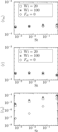
Figure 1: Mean dissipation and injection rates as a function of the Stokes and Weissenberg numbers. Upper picture: mean energy injection rate due to shear flow forcing $\langle\varepsilon_{\mathrm{in}}\rangle$. Mid panel: mean energy dissipation rate $\langle\varepsilon\rangle$. Lower panel: mean dissipation rate which arises from the coupling to the dumbbell ensemble $\langle\varepsilon_{\mathrm{p}}\rangle$. The Reynolds number is $\mathrm{Re}=800$. The case with $F_{\mathrm{el}}=0$ is for the case without spring force and stands for a shear flow with dispersed inertial particles.

Figure 1 shows the three mean rates as a function of the Stokes number for two Weissenberg numbers $\mathrm{Wi}=20,100$. The mean energy dissipation rate $\langle\varepsilon\rangle$ and the mean energy injection rate $\langle\varepsilon_{\mathrm{in}}\rangle$ are of the same order of magnitude for all cases. They remain nearly unchanged with respect to Weissenberg number, which indicates that the effect of the dumbbell ensemble on the macroscopic flow properties is small. Nevertheless, one observes a slight increase of the mean energy injection rate $\langle\varepsilon_{\mathrm{in}}\rangle$ with respect to $\mathrm{St}$ going in line with a decrease of $\langle\varepsilon\rangle$ (see upper and mid panel of Fig. 1). Recall that the energy injection rate will be maximal for the laminar case, i.e. for ${\bm{u}}\parallel{\bm{f}}$. The trend of the data indicates that the streamwise flow component relaminarizes slightly with growing inertia. The lower panel of the same figure shows the findings for the dissipation due to polymer stretching $\langle\varepsilon_{\mathrm{p}}\rangle$. As an additional energy dissipation mechanism, it consumes injected energy which goes into the elastic energy budget of the dumbbell ensemble. The rate $\langle\varepsilon_{\mathrm{p}}\rangle$ grows in magnitude with respect to both parameters, the Stokes and Weissenberg number. For $\mathrm{Wi}=3$, the dumbbells are not significantly extended and no clear trend of $\langle\varepsilon_{\mathrm{p}}\rangle$ with $\mathrm{St}$ could be observed. The dissipation rate $\langle\varepsilon_{\mathrm{p}}\rangle$ is significantly smaller in comparison to the runs with larger $\mathrm{Wi}$.

In order to estimate the maximum feedback of the dumbbells on the flow, we performed an “academic experiment” for our system by tethering one of the two beads of a dumbbell at a fixed position. The dumbbells get then stretched more efficiently and undergo strong conformational fluctuations. Figure 2 illustrates their dramatic effect on the total kinetic energy. We compare the freely draining case with the tethered one and observe a significant decrease of the kinetic energy. An inspection of the flow structures indicates that the turbulent fluctuations are supressed almost completely. The flow becomes basically laminar. The magnitude of the feedback for freely draining dumbbells will always remain significantly below this artifical limit with tethered dumbbells.

III.2 Reynolds stresses

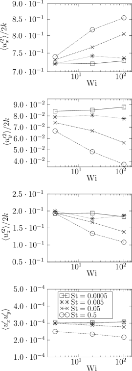
Figure 3: Reynolds stresses $\langle u_{i}^{\prime}u_{j}^{\prime}\rangle$ normalized by the turbulent kinetic energy $k=\langle(u_{i}^{\prime})^{2}\rangle/2$ as a function of the Weissenberg and Stokes numbers. From top to bottom: streamwise fluctuations, fluctuations in shear direction, spanwise fluctuations, and shear stress. The Reynolds number is $\mathrm{Re}=800$.

Figure 3 shows the four non-vanishing components of the Reynolds stress tensor $\langle u_{i}^{\prime}u_{j}^{\prime}\rangle/(2k)$ where $k=\langle(u_{i}^{\prime})^{2}\rangle/2$ is the turbulent kinetic energy (TKE). The moments are averages over the whole simulation volume for a sequence of about 100 statistically independent snapshots of the time evolution of the shear flow. The results can be summarized to the following trends. For the two smallest Stokes numbers, no dependence on the Weissenberg number is observed. For $\mathrm{St}=0.05$ and 0.5, the mean streamwise fluctuations are enhanced while the remaining components of the Reynolds stress tensor decrease as a function of $\mathrm{Wi}$. This finding is in agreement with observations in a Kolmogorov flow by Boffetta et al. Boffetta2005

Similar to the friction factor for a turbulent pipe Schlichting , we can define a friction factor for the present flow where the applied pressure gradient term has to be substituted by an amplitude of the static volume forcing profile ${\bm{f}}$ that sustains the laminar cosine flow profile. Consequently,

$$c_{f}=\frac{2FL_{y}}{\langle u_{x}(y=L_{y})\rangle^{2}}\,.$$ (27)

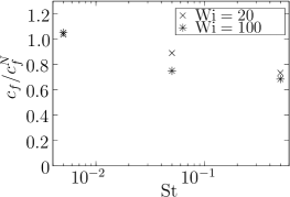
Figure 4: Ratio of friction factors as a function of $\mathrm{St}$ for the largest $\mathrm{Wi}$. The friction factor for the fluid with the dispersed dumbbells is $c_{f}$ (cf. Eq. (27)). The quantity $c_{f}^{N}$ is the friction factor of the Newtonian fluid.

Since ${\bm{f}}(y)=-\sqrt{2}\pi^{2}/(4\nu)\cos(\pi y/2){\bm{e}}_{x}$, we take $F=f_{x}(y=L_{y})=\sqrt{2}\pi^{2}/(4\nu)$. A similar definition was suggested for a Kolmogorov flow which is also driven by a volume forcing.Boffetta2005 Drag reduction by dispersed dumbbells would go in line with a decrease of the dimensionless measure $c_{f}$ below the Newtonian value $c_{f}^{N}$. For the smallest Stokes number, the ratio goes to about unity. The slight overshoot is attributed to the strong variations of the streamwise velocity at the free-slip planes. Figure 4 indicates a reduction by $20\%-25\%$ at $\mathrm{St}=0.05,0.5$ and for the larger Weissenberg numbers. The series with $\mathrm{Wi}=3$ gave $c_{f}\simeq c_{f}^{N}$.

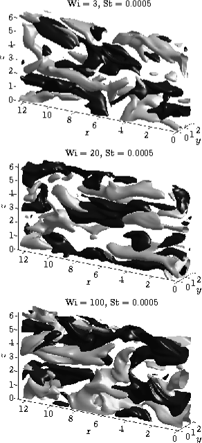
Figure 5: Isosurface plot of the fluctuations of the streamwise turbulent velocity component $u_{x}^{\prime}$. The snapshots are for $\mathrm{Re}=800$ and $\mathrm{St}=0.0005$. The isolevels are for $\pm 0.04$ in each case.

An important structural ingredient of shear flows are the asymmetric fluctuations of the three diagonal elements of the Reynolds stress tensor. The streamwise fluctuations $\langle(u_{x}^{\prime})^{2}\rangle$ are spatially arranged in streamwise streaks which interact with streamwise vortices in a so-called regeneration cycle of coherent structures. This cycle is sustained by the non-normal amplification mechanism.Waleffe1997 ; Grossmann2001 The impact of long-chained polymers on the extension of the streamwise streaks has been demonstrated in experiments White2004 and numerical simulations.Stone2004 ; Dubief2004 While streamwise fluctuations were found to increase, the fluctuations in shear and spanwise directions decreased. This is in line with our observations as discussed above. In Fig. 5, we show isolevels of the streamwise turbulent fluctuations for opposite sign at $\mathrm{Wi}=3,20,100$. Although not very pronounced, a slight increase in the connectivity and extension of the streamwise streaks can be observed with increasing Weissenberg number.

As we can see, the statistics of macroscopic turbulent properties is affected only slightly by the dispersed FENE-dumbbells. Their impact increases with Weissenberg number as well as with Stokes number. In order to rule out that particle inertia dominates the discussed trends of our studies, we considered the case of dispersed beads in the same flow at the same Stokes numbers. This is achieved by switching off the elastic spring force, i.e. $F_{\mathrm{el}}=0$. The Stokes friction force remained as the only force. The quantity ${\bm{f}}_{\mathrm{p}}$ models then the feedback of the particles on the flow. We added the statistical means of injection and dissipation rates as a function of the Stokes number for this case to Fig. 1. While the mean injection and mean dissipation rates are of the same magnitude, the dissipation due to particle feedback is orders of magnitude smaller in comparison to the polymer feedback, except for the largest $\mathrm{St}$. In addition, we found no clear trends for the Reynolds stress components as a function of $\mathrm{St}$.

IV Small-scale properties

IV.1 Extensional and angular statistics of dumbbells

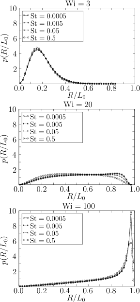
Figure 6: Probability density function (PDF) of the extension $R$ normalized by the contour length $L_{0}$. Three different Weissenberg numbers are shown. The Stokes numbers of the data are indicated in the legend. Data are for $\mathrm{Re}=800$.

The finite extensibility of the dumbbells will affect the shape of the probability density function (PDF) of $R$, which is supported on scales smaller than $L_{0}$ only. Figure 6 reports our findings for $p(R)$ for different Weissenberg and Stokes numbers. For the lowest Weissenberg number, $\mathrm{Wi}=3$, the majority of the dumbbells remains at the extension of about the Kolmogorov length $\eta_{\mathrm{K}}$. This picture changes for larger values of $\mathrm{Wi}$. At $\mathrm{Wi}=100$, the majority of the ensemble is stretched to almost $L_{0}$, which manifests in the sharp maximum at $R\lesssim L_{0}$. Qualitatively, the change of the shapes of the PDFs with increasing $\mathrm{Wi}$ agrees well with experimental findings Steinberg2005 and analytical studies Celani2005 ; Chertkov2005 for the coil-stretch transition in random flows. The trends with the Stokes number remain small in all cases. However, the data show that growing particle inertia suppresses the stretching to very extended molecules since the response time of the molecules to the variation of the structures increases (see e.g. mid panel of Fig. 6).

As we have seen in the last section, the fluctuations of the turbulent velocity field in the shear flow vary strongly from one space direction to another (see e.g. Fig. 3). The major contribution is contained in the streamwise component $\langle(u_{x}^{\prime})^{2}\rangle$ parallel to the direction of the mean turbulent flow. This suggests an investigation of the angular statistics of the polymers since their stretching can be expected to become anisotropic as well. The following dumbbell coordinate system will be used therefore throughout this text: $R_{x}=R\cos\varphi\cos\theta$, $R_{y}=R\sin\varphi\cos\theta$, and $R_{z}=R\sin\theta$, where $R$ is the distance between both beads. The notation differs from conventional spherical coordinates, but has the advantage of giving perfect alignment with the outer mean flow direction for $\varphi=\theta=0$. $\varphi$ is the azimuthal angle and $\theta$ the polar angle. While the azimuthal angle always remains in the shear plane that is spanned by the streamwise and shear directions, the polar angle $\theta\neq 0$ indicates a dumbbell orientation out of this plane.

Davoudi and Schumacher Schumacher2006 discussed the statistics of both angles as a function of the Weissenberg number for passively advected Hookean dumbbells. The PDF of the polar angle was found to remain symmetric and to be less sensitive with respect to variations of $\mathrm{Wi}$. Our focus will be therefore on the statistics of the azimuthal angle $\varphi$ which can take values between $-\pi/2$ and $\pi/2$. The asymmetry between both quadrants is quantified by the following measure for the PDF $p(\varphi)$:

$$A(\varphi)=p(\varphi)-p(-\varphi)\,,$$ (28)

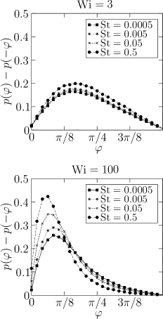
Figure 7: Asymmetry of the probability density function (PDF) of the azimuthal angle $\varphi$. It is defined as $A(\varphi)=p(\varphi)-p(-\varphi)$. The upper panel shows the data for $\mathrm{Wi}=3$ and four different Stokes numbers. The lower panel shows the data for $\mathrm{Wi}=100$ and four different Stokes numbers. The analysis is for $\mathrm{Re}=800$.

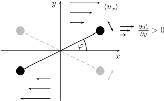
Figure 8: Sketch of the orientation of a dumbbell in the turbulent shear flow. The mean turbulent flow profile is indicated. The dark-colored dumbbell stands for the preferentially oriented one while the gray-colored orientation is less probable. This orientation asymmetry leads to the asymmetry in the angular distribution as given in Fig. 7.

with $\varphi\in[0,\pi/2]$. The measure $A(\varphi)$ is plotted for two Weissenberg numbers in Fig. 7. A pronounced maximum of $A(\varphi)$ implies that the dumbbells are preferentially slightly tilted in the direction of shear, away from the mean flow direction (see an illustration in Fig. 8). We find that with increasing Weissenberg number the asymmetry of the angular distribution grows in magnitude. The same trend holds when the Stokes number grows at fixed Weissenberg number. In each case, the graph of $A(\varphi)$ shows an increasingly sharper maximum, which is shifted towards smaller $\varphi$. Fluctuations of the dumbbells in the vicinity of $\varphi=0$ are enhanced while the tails for very large $\varphi$ are depleted. Growing inertia amplifies this trend. Once the dumbbells are aligned along the mean flow they remain in this orientation for longer periods of their evolution.

IV.2 Velocity gradient statistics

Since the polymer dynamics takes place at the smallest scales of the turbulent flow, we study the impact of the dumbbells on the small-scale statistical properties of the flow in the following. Recent experimental and numerical studies in simple Newtonian shear flows indicate that in particular the statistics of the transverse derivative of the streamwise turbulent velocity component $\partial u_{x}^{\prime}/\partial y$ is a sensitive measure for detecting deviations from local isotropy in homogeneous or nearly homogeneous shear flows.Warhaft2002 ; Schumacher2003 ; Biferale2005 In a shear flow with a mean shear rate $S>0$, one expects a positive value for derivative skewness and other higher odd order moments which are defined as

$$M_{2n+1}(\partial u_{x}^{\prime}/\partial y)=\frac{\langle(\partial u_{x}^{\prime}/\partial y)^{2n+1}\rangle}{\langle(\partial u_{x}^{\prime}/\partial y)^{2}\rangle^{n+1/2}}\,.$$ (29)

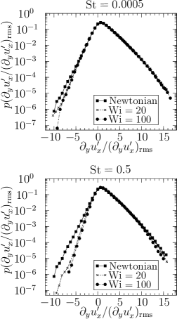
Figure 9: Probability density function (PDF) of the transverse velocity gradient of the streamwise turbulent fluctuations, $\partial u_{x}^{\prime}/\partial y$. The Newtonian case is compared with the two larger values of the Weissenberg number at $\mathrm{St}=5\times 10^{-4}$ and 0.5, respectively. The data are for $\mathrm{Re}=800$.

The derivative moments would be exactly zero in a perfectly isotropic flow. Their non-zero magnitudes indicate that velocity gradient fluctuations of the streamwise component along the direction of the outer shear gradient are more probable than the ones in the opposite direction. It can be expected that the asymmetry in the angular distribution, which we discussed above, will have an impact on the statistics of exactly these gradient fluctuations. Figure 9 reports our findings for the PDF of the transverse derivative, which has been normalized by its root mean square value for all cases. We observe in both figures a depletion of the left hand tail, which stands exactly for the velocity gradient fluctuations opposite to the direction of the mean shear. The results suggest that the preferential orientation fluctuations of the dumbbells at azimuthal angles $\varphi>0$ go in line with a depletion of the negative tail of the PDF of the transverse derivative. As sketched in Fig. 8, negative transverse gradients would be amplified by prefential orientations with $\varphi<0$ which correspond to the dumbbell colored in gray. The findings are consistent with our observations on the $\varphi$-statistics. They can also be rationalized (but not explained) when considering the equation for the Brownian dynamics of the FENE dumbbell Oettinger1996

$$\frac{\mbox{d}{\bm{R}}}{\mbox{d}t}={\bm{R}\cdot\nabla u}-\frac{{\bm{R}}}{2\tau(1-R^{2}/L_{0}^{2})}+\sqrt{\frac{R_{0}^{2}}{\tau}}{\bm{\xi}}_{\bm{R}}\,.$$ (30)

In the plane shear flow geometry the component $R_{x}$ along the mean flow direction is of particular interest. Since we are interested in stretched dumbbells with $R_{x}>R_{0}$ and in $\mathrm{Wi}>1$ we neglect contributions from the spring force and the noise for a moment. With the Reynolds decomposition (7) we get

$$\frac{\mbox{d}R_{x}}{\mbox{d}t} \simeq \left(S+\frac{\partial u_{x}^{\prime}}{\partial y}\right)R_{y}+\left(\frac{\partial u_{x}^{\prime}}{\partial x}\right)R_{x}+...\,,$$ (31)

$$\frac{\mbox{d}R_{y}}{\mbox{d}t} \simeq \left(\frac{\partial u_{y}^{\prime}}{\partial y}\right)R_{y}+\left(\frac{\partial u_{y}^{\prime}}{\partial x}\right)R_{x}+...$$ (32)

The important term is the first term on the r.h.s. of (31). The other three contributions will behave as noise terms. Fluctuating gradients $\partial u_{x}^{\prime}/\partial y$ along $S{\bm{e}}_{y}$ lead to a more rapid growth of $R_{x}$ (for an angle $\varphi>0$) and a prefered alignment with the mean flow. This causes a more rapid decrease of $R_{y}$ and consequently of $R_{x}$ via (31). The dumbell can be kicked afterwards again to larger $\varphi$ values and transfers momentum to the flow which corresponds exactly to a local patch of $\partial u_{x}^{\prime}/\partial y>0$ (see also Fig. (8)). Then $R_{y}$ grows and this whole cycle starts anew. Small scale gradients with the opposite sign diminish the total shear in the surrounding of the dumbbell and cause a less efficient stretching and cycle. Clearly, this picture omits some important features such as the tumbling of the dumbbells.

The depletion of gradient fluctuations goes in line with experimental observations by Liberzon et al. Liberzon2005 ; Liberzon2006 The authors found e.g. that the enstrophy production became anisotropic when polymers are added to the fluid. This quantity is directly related to transverse gradient components discussed here.

IV.3 Invariants of the velocity gradient tensor and dumbbell extension

The efficient stretching of the dumbbells is connected to particular local flow topologies. They are related to the three eigenvalues $\lambda_{i}$ of the velocity gradient tensor or the corresponding three velocity gradient tensor invariants, which are denoted as $I_{1}$, $I_{2}$, and $I_{3}$. The eigenvalues of the velocity gradient tensor $\partial u_{i}^{\prime}/\partial x_{j}$ result as zeros of the following third-order characteristic polynomialDavidson

$$\lambda^{3}-I_{1}\lambda^{2}+I_{2}\lambda-I_{3}=0\,.$$ (33)

For an incompressible flow ,

$$I_{1} = \lambda_{1}+\lambda_{2}+\lambda_{3}=\mbox{Tr}\left(\frac{\partial u_{i}^{\prime}}{\partial x_{j}}\right)=0\,,$$

$$I_{2} = \lambda_{1}\lambda_{2}+\lambda_{2}\lambda_{3}+\lambda_{3}\lambda_{1}=-\frac{1}{2}\,\frac{\partial u_{i}^{\prime}}{\partial x_{j}}\,\frac{\partial u_{j}^{\prime}}{\partial x_{i}}\,,$$

$$I_{3} = \lambda_{1}\lambda_{2}\lambda_{3}=\mbox{det}\left(\frac{\partial u_{i}^{\prime}}{\partial x_{j}}\right)=\frac{1}{3}\,\frac{\partial u_{i}^{\prime}}{\partial x_{j}}\,\frac{\partial u_{j}^{\prime}}{\partial x_{k}}\,\frac{\partial u_{k}^{\prime}}{\partial x_{i}}\,.$$ (34)

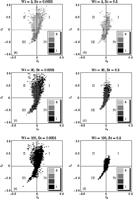
Figure 10: Relation between the extension of the dumbbells and the local velocity gradient at the center of mass of the dumbbells. The local flow topology that is related to the velocity gradient is quantified by the second and third invariants $I_{2}$ and $I_{3}$ (see eqns. (34) for the definition). Quadrant I stands for vortex stretching, II for vortex compression, III for bi-axial strain, and IV for uniaxial strain, respectively. The gray color coding of the bins for $0<R/L_{0}<0.25$, $0.25\leq R/L_{0}<0.5$, $0.5\leq R/L_{0}<0.75$, $0.75\leq R/L_{0}\leq 1$ is indicated by the legend for each figure. Data are for $\mathrm{Re}=800$.

The remaining coefficients of (33) are therefore $I_{2}$ and $I_{3}$, which span the $I_{3}-I_{2}$ parameter plane. The scatter plots for turbulent flows result in a typical skewed teardrop shape. With our definitions given above the following crude classification scheme can be given. For $I_{2}>0,I_{3}>0$ vortex stretching is present corresponding to $\lambda_{1}=a,\lambda_{2,3}=-a\pm\mbox{i}b$ (first quadrant); for $I_{2}>0,I_{3}<0$ vortex compression is present corresponding to $\lambda_{1}=-a,\lambda_{2,3}=a\pm\mbox{i}b$ (second quadrant). The cases $I_{3}<0$ are associated with bi-axial strain for $I_{2}<0$ (third quadrant) corresponding to $\lambda_{1}=a,\lambda_{2}=b,\lambda_{3}=-(a+b)$ and with uniaxial strain at $I_{2}>0$ (fourth quadrant) corresponding to $\lambda_{1}=a,\lambda_{2}=-b,\lambda_{3}=-(a-b)$. Constants $a$ and $b$ are larger than zero in all cases. Figure 10 relates the extension of the dumbbells to the corresponding local velocity gradients in the $I_{3}-I_{2}$ plane (and consequently to the existing local flow topology). The invariants of the velocity gradient were evaluated in the center of mass of each dumbbell. The typical teardrop shape for the turbulence data in the parameter plane is detected.

Our findings can be summarized as follows. Strongly stretched dumbbells go in line with the largest excursions of the gradients in the $I_{3}-I_{2}$ plane. The longest dumbbells are found preferentially in regions where vortex stretching or bi-axial strain dominate the local flow topology. The preferential stretching by bi-axial strain was discussed already for the passive advection of FENE dumbbells in a minimal flow unit.Terrapon2004 It corresponds to the scenario that different parts of the dumbbell get pulled by counterstreaming streamwise streaks. The preferential extension close to vortex stretching means that the polymers are pulled around streamwise vortices. This point was outlined in Ref. Dubief2004 on the basis of an analysis of the energetics of viscoelastic turbulence. Here, we find both in a common description based on the analysis of the full velocity gradient tensor, i.e. the symmetric strain tensor plus the anti-symmetric vorticity tensor. We do also observe that the area of the teardrop shape shrinks with increasing Stokes number. This indicates that the small-scale velocity gradients are supressed in magnitude, which goes in line with more limited excursions across the $I_{3}-I_{2}$ plane and a relaminarization of the turbulence. Again, this goes in line with very recent experimental observations by Liberzon et al.Liberzon2006

V Summary and discussion

The presented numerical studies aimed at connecting a macroscopic description for the Newtonian turbulent shear flow to the mesoscopic description of an ensemble of FENE dumbbells which are advected in such flow. The momentum transfer of the dumbbells with the fluid is implemented by an additional volume forcing in the Navier-Stokes equations. In numerical terms, pseudospectral simulations for the solvent are coupled to a system of stochastic nonlinear ordinary equations in order to model a viscoelastic fluid.

For the accessible parameters we found slight modifications of the macroscopic flow structures and mean statistical properties only. This was demonstrated for the global energy balance and the mean components of the Reynolds stress tensor. We conclude that dumbbell inertia effects are present, but remain subleading in comparison to the elastic properties. For the present viscoelastic flow a drag reduction of up to 20% is achieved. The microscopic properties of turbulence were found to be more sensitive with respect to the Weissenberg number. The statistics of the azimuthal angle $\varphi$ is consistent with former findings for elastic Hookean dumbbells. Schumacher2006 A growing number of dumbbells becomes increasingly aligned with the mean flow direction. The feedback of the FENE dumbbells on the small-scale properties of turbulence is demonstrated for two gradient measures, the PDF of the transverse derivative of the turbulent streamwise velocity component $\partial u_{x}^{\prime}/\partial y$ and the diminished scattering of the velocity gradient invariants ampiltudes in the $I_{3}-I_{2}$ plane with increasing $\mathrm{Wi}$. The asymmetry of the PDF $p(\partial u_{x}^{\prime}/\partial y)$ is found to increase with increasing $\mathrm{Wi}$. Furthermore, we determined that strongly stretched dumbbells can be found close to vortex stretching or biaxial strain topologies of the advecting shear flow.

The present study should be considered as a first step for such class of hybrid models. One difference to the situation in a dilute polymer solution is the relatively large Stokes number that had to be taken. Our dispersed dumbbells behave in parts like deformable particles rather than polymer chains. Frequently, heavier quasi-particles are used for the study of turbulence in particle-ladden flows.Bosse2006 Extensions of our investigations will have to go into two directions. Firstly, it is desirable that larger spectral resolutions, like the ones in Ref. Schumacher2006 , are achieved. This will require a fully parallel implementation of the current numerical scheme. Larger computational grids and higher Reynolds numbers will give us the opportunity to decrease the ratio $R_{0}/\eta_{\mathrm{K}}$ and to increase $L_{0}/R_{0}$ to more realistic values. Secondly, eq. (21) implies the efforts that have to be taken in order to approach the situation in a polymer solution. Decreasing values of $R_{0}$ and $\mathrm{St}$ have to be compensated by $n_{\mathrm{p}}$, e.g., a reduction of both – $R_{0}$ and $\mathrm{St}_{\eta}$ – by an order of magnitude requires an increase of the concentration (or number density) by a power of 5/2. Once such operating point is reached, the time scale argument which is thought to be important for the drag reduction effect, can also be studied.Lumley1969 Finally, a recent work by Vincenzi and co-workers Vincenzi2006 provides an interesting ansatz for modelling the polymer dynamics. The authors studied a conformation-dependent Stokes drag coefficient that caused a significant dynamical slow-down of the coil-stretch transition in steady elongational and random flows. The test of these ideas in turbulent shear flows is still to be done.

Appendix A Semi-implicit integration scheme for dumbbells

The FENE dumbbells consist of two beads at positions ${\bm{x}}_{1}(t)$ and ${\bm{x}}_{2}(t)$ which are connected by a nonlinear elastic spring. The velocities of the advecting flow at both beads are denoted by ${\bm{u}}_{1}$ and ${\bm{u}}_{2}$, respectively. Note that these velocities coincide with $\dot{\bm{x}}_{1}$ and $\dot{\bm{x}}_{2}$, respectively, for $\mathrm{St}=0$ only. Since the beads are usually found between mesh vertices, the values for ${\bm{u}}_{1}$ and ${\bm{u}}_{2}$ have to be determined by trilinear interpolation from the known velocity vectors at the neighboring grid sites. The dynamical equations for the dumbbells are set up in relative and center-of-mass coordinates. The relative coordinate (or separation) vector of the dumbbell is given by

$${\bm{R}}(t)={\bm{x}}_{2}(t)-{\bm{x}}_{1}(t)\,.$$ (35)

The center-of-mass coordinate vector is given by

$${\bm{r}}(t)=\frac{1}{2}({\bm{x}}_{1}(t)+{\bm{x}}_{2}(t))\,.$$ (36)

The velocities which are assigned with the relative and center-of mass coordinates are denoted as ${\bm{V}}$ and ${\bm{v}}$, respectively. The Newtonian equations for the dynamics of the FENE dumbbells in dimensionless form, which follow then from (9)-(12) with the definitions (3) and (2), are given by

$$\frac{\mbox{d}\tilde{\bm{r}}}{\mbox{d}t} = \tilde{\bm{v}}\,,$$ (37)

$$\frac{\mbox{d}\tilde{\bm{v}}}{\mbox{d}t} = \frac{1}{\mathrm{St}}\left[-\tilde{\bm{v}}+\frac{1}{2}(\tilde{\bm{u}}_{1}+\tilde{\bm{u}}_{2})+\frac{R_{0}}{2L\sqrt{\mathrm{Wi}}}\tilde{\bm{\xi}}_{\bm{r}}\right]\,,$$ (38)

$$\frac{\mbox{d}\tilde{\bm{R}}}{\mbox{d}t} = \tilde{\bm{V}}\,,$$ (39)

$$\frac{\mbox{d}\tilde{\bm{V}}}{\mbox{d}t} = \frac{1}{\mathrm{St}}\left[-\tilde{\bm{V}}+(\tilde{\bm{u}}_{2}-\tilde{\bm{u}}_{1})-\frac{\tilde{\bm{R}}}{2\mathrm{Wi}\left(1-\tilde{R}^{2}L^{2}/L_{0}^{2}\right)}+\frac{R_{0}}{\sqrt{\mathrm{Wi}}\,L}\tilde{\bm{\xi}}_{\bm{R}}\right]\,.$$ (40)

For the following, we omit the tilde symbol for the dimensionless quantities. The predictor values of the center-of-mass vector ${\bm{r}}$ and the distance vector ${\bm{R}}$ are calculated by an explicit Euler step whereas the corresponding velocities are treated by an implicit Euler step, giving

$${\bm{r}}^{*} = {\bm{r}}^{l}+\Delta t{\bm{v}}^{l}\,,$$ (41)

$${\bm{v}}^{*} = \frac{1}{\mathrm{St}+\Delta t}\left[\mathrm{St}\,{\bm{v}}^{l}+\frac{1}{2}({\bm{u}}_{1}^{l}+{\bm{u}}_{2}^{l})\Delta t+\frac{R_{0}}{2L\sqrt{\mathrm{Wi}}}\Delta{\bm{w}}^{l}\right]\,,$$ (42)

$${\bm{R}}^{*} = {\bm{R}}^{l}+\Delta t{\bm{V}}^{l}\,,$$ (43)

$${\bm{V}}^{*} = \frac{1}{\mathrm{St}+\Delta t}\left[\mathrm{St}\,{\bm{V}}^{l}+({\bm{u}}_{2}^{l}-{\bm{u}}_{1}^{l})\Delta t-\frac{{\bm{R}}^{l}}{2\mathrm{Wi}\left(1-(R^{l})^{2}L^{2}/L_{0}^{2}\right)}\,\Delta t+\frac{R_{0}}{L\sqrt{\mathrm{Wi}}}\Delta{\bm{W}}^{l}\right]\,.$$ (44)

The corrector step for the center-of-mass and distance vectors is given as

$${\bm{r}}^{l+1} = {\bm{r}}^{l}+\frac{1}{2}({\bm{v}}^{*}+{\bm{v}}^{l})\Delta t$$ (45)

$${\bm{v}}^{l+1} = \frac{1}{\mathrm{St}+\Delta t}\,\Bigg{[}\frac{1}{2}\left(\mathrm{St}\,{\bm{v}}^{*}+\frac{1}{2}({\bm{u}}^{*}_{1}+{\bm{u}}^{*}_{2})\Delta t+\mathrm{St}\,{\bm{v}}^{l}+\frac{1}{2}({\bm{u}}^{l}_{1}+{\bm{u}}^{l}_{2})\Delta t\right)+$$ (46)

$$\frac{R_{0}}{2L\sqrt{\mathrm{Wi}}}\Delta{\bm{W}}^{l}\Bigg{]}$$

$${\bm{R}}^{l+1} = {\bm{R}}^{l}+\frac{1}{2}({\bm{V}}^{l}+{\bm{V}}^{l+1})\Delta t$$ (47)

$${\bm{V}}^{l+1} = \frac{1}{\mathrm{St}+\Delta t}\,\Bigg{[}\frac{1}{2}\Bigg{(}\mathrm{St}\,{\bm{V}}^{*}+({\bm{u}}^{*}_{2}-{\bm{u}}^{*}_{1})\Delta t+\mathrm{St}\,{\bm{V}}^{l}+({\bm{u}}^{l}_{2}-{\bm{u}}^{l}_{1})\Delta t-$$ (48)

$$\frac{{\bm{R}}^{l+1}}{2\mathrm{Wi}\left(1-({\bm{R}}^{l+1})^{2}L^{2}/L_{0}^{2}\right)}\,\Delta t-\frac{{\bm{R}}^{l}}{2\mathrm{Wi}\left(1-({\bm{R}}^{l})^{2}L^{2}/L_{0}^{2}\right)}\,\Delta t\Bigg{)}+$$

$$\frac{R_{0}}{L\sqrt{\mathrm{Wi}}}\Delta{\bm{W}}^{l}]\,.$$

Note that the corrector step for the distance vector is semi-implicit in the velocity in order to avoid stiffness of the equation system at small Stokes numbers. The corrector step for the distance velocity ${\bm{V}}$ has to be semi-implicit in the separation vector ${\bm{R}}$ due to the finite extensibility of the dumbbells.Oettinger1996 When inserting (48) into (47) one gets

$$\left(1+\frac{(\Delta t)^{2}}{8\mathrm{Wi}\,(\mathrm{St}+\Delta t)\left(1-({\bm{R}}^{l+1})^{2}L^{2}/L_{0}^{2}\right)}\right){\bm{R}}^{l+1}={\bm{A}}\,,$$ (49)

where the abbrevation ${\bm{A}}$ contains terms only which are known. By taking the norm of (49) one ends up with a cubic polynomial for $R^{l+1}$. The formula for the “casus irreducibilis” of three real solutions of the polynomial goes back to F. Viète Vieta and yields directly the unique solution for $R=|{\bm{R}}|$ between 0 and $L_{0}$. From (49) follows now

$${\bm{R}}^{l+1}=R^{l+1}\frac{\bm{A}}{A}\,.$$ (50)

This value is inserted into (48) which completes the corrector step.

Figure 2: Comparison of the kinetic energy for two cases at $\mathrm{Wi}=20$ and $\mathrm{St}=0.05$: for the tethered case one bead of each dumbbell is fixed at a grid site while the second bead can fluctuate. The freely draining case is the usual situation which allows the free motion of the dumbbells through the turbulent flow volume. The Reynolds number is $\mathrm{Re}=400$.

References

- (1) J. L. Lumley, “Drag reduction by additives,” Annu. Rev. Fluid Mech. 1, 367 (1969).
- (2) B. A. Toms, “Observations on the flow of linear polymer solutions through straight tubes at large Reynolds numbers,” in Proceedings of the International Congress on Rheology (Holland 1948), Vol. 2, pp. 135-141 North-Holland, Amsterdam (1949).
- (3) P. S. Virk, “Drag reduction fundamentals,” AIChE J. 21, 625 (1975).
- (4) G. H. McKinley and T. Sridhar, “Filament-stretching rheometry of complex fluids,” Annu. Rev. Fluid Mech. 34, 375 (2002).
- (5) R. G. Larson, “The rheology of dilute solutions of polymers: Progress and problems,” J. Rheol. 49, 1 (2005).
- (6) M. Doi, Introduction to polymer physics, Cambridge University Press, Cambridge, 1996.
- (7) R. Benzi, E. De Angelis, V. S. L‘vov, I.Procaccia, and V. Tiberkevich, “Maximum drag reduction asymptotes and the cross-over to the Newtonian plug,” J. Fluid Mech. 551, 185 (2006).
- (8) M. D. Warholic, H. Massah, and T. J. Hanratty, “Influence of drag-reducing polymers on turbulence: effects of Reynolds number, concentration and mixing,” Exp. Fluids 27, 461 (1999).
- (9) K. R. Sreenivasan and C. M. White, “The onset of drag reduction by dilute polymer additives and the maximum drag reduction asymptote,” J. Fluid Mech. 409, 149 (2000).
- (10) C. M. White, V. S. R. Somandepalli, and M. G. Mungal, “The turbulence structure of drag reduced boundary layer flow,” Exp. Fluids 36, 62 (2004).
- (11) R. B. Bird, R. C. Amstrong, and O. Hassager, Dynamics of polymeric liquids, John Wiley & Sons, New York, 1987.
- (12) R. Sureshkumar, A. N. Beris, and R. A. Handler, “Direct numerical simulation of the turbulent channel flow of a polymer solution,” Phys. Fluids 9, 743 (1997).
- (13) P. Ilg, E. De Angelis, I. V. Karlin, C. M. Casciola, and S. Succi, “Polymer dynamics in wall turbulent flow,” Europhys. Lett. 58, 616 (2002).
- (14) B. Eckhardt, J. Kronjäger, and J. Schumacher, “Stretching of polymers in a turbulent enviroment,” Comp. Physics Comm. 147, 538 (2002).
- (15) C. D. Dimitropolous, Y. Dubief, E. S. G. Shaqfeh, P. Moin, and S. K. Lele, “Direct numerical simulation of polymer-induced drag reduction in a turbulent shear flow,” Phys. Fluids 17, 011705 (2005).
- (16) T. Vaithianathan and L. R. Collins, “Numerical approach to simulating turbulent flow of a viscoelastic polymer solution,” J. Comp. Phys. 187, 1 (2003).
- (17) C. R. Doering, B. Eckhardt, and J. Schumacher, “Failure of energy stability in Oldroyd-B fluids at arbitrarily low Reynolds numbers,” J. Non-Newtonian Fluid Mech. 135, 92 (2006).
- (18) H. Temmen, H. Pleiner, M. Liu, and H. R. Brand, “Convective nonlinearity in non-Newtonian fluids,” Phys. Rev. Lett. 84, 3228 (2000).
- (19) A. N. Beris, M. D. Graham, I. Karlin, and H.-C. Öttinger, “Comment on Convective nonlinearity in non-Newtonian fluids,” Phys. Rev. Lett. 86, 744 (2001).
- (20) H. Temmen, H. Pleiner, M. Liu, and H. R. Brand, “Temmen et al. reply,” Phys. Rev. Lett. 86, 745 (2001).
- (21) H.-C. Öttinger, Stochastic processes in polymeric fluids, Springer Verlag, Berlin, 1996.
- (22) A. Celani, A. Puliafito, and K. Turitsyn, “Polymers in linear shear flow: a numerical study,” Europhys. Lett. 70, 464 (2005).
- (23) J. S. Hur, E. S. G. Shaqfeh, H. P. Babcock, D. E. Smith, and S. Chu, “Dynamics of dilute and semidilute DNA solutions in the start-up of shear flow,” J. Rheol. 45, 421 (2001).
- (24) P. A. Stone and M. D. Graham, “Polymer dynamics in a model of the turbulent buffer layer,” Phys. Fluids 15, 1247 (2003).
- (25) V. E. Terrapon, Y. Dubief, P. Moin, E. S. G. Shaqfeh, and S. K. Lele, “Simulated polymer stretch in a turbulent flow using Brownian dynamics,” J. Fluid Mech. 504 61 (2004).
- (26) B. H. Zimm, “Dynamics of polymers in dilute solution - viscoelasticity, birefringence and dielectric loss,” J. Chem. Phys. 24, 269 (1956).
- (27) A. Celani, S. Musacchio, and D. Vincenzi, “Polymer transport in random flow,” J. Stat. Phys. 118, 531 (2005).
- (28) J. Davoudi and J. Schumacher,“Stretching of polymers around the Kolmogorov scale in a turbulent shear flow,” Phys. Fluids 18, 025103 (2006).
- (29) K. D. Squires and J. K. Eaton, “Particle response and turbulence modification in isotropic turbulence,” Phys. Fluids A 2, 1191 (1990).
- (30) S. Elghobashi and G. C. Truesdell, “On the two-way interaction between homogeneous turbulence and dispersed solid particles. I: Turbulence modification,” Phys. Fluids A 5, 1790 (1993).
- (31) T. Bosse, L. Kleiser, and E. Meiburg, “Small particles in homogeneous turbulence: Settling velocity enhancement by two-way coupling,” Phys. Fluids 18, 027102 (2006).
- (32) I. M. Mazzitelli, D. Lohse, and F. Toschi, “On the relevance of the lift force in bubbly turbulence,” J. Fluid Mech. 488, 283 (2003).
- (33) P. Ahlrichs and B. Dünweg, “Simulation of a single polymer chain in solution by combining lattice Boltzmann and molecular dynamics,” J. Chem. Phys. 111, 8225 (1999).
- (34) J. D. Schieber and H.-C. Öttinger, “The effect of bead inertia on the Rouse model,” J. Chem. Phys. 89, 6972 (1988).
- (35) J. Schumacher and B. Eckhardt, “Evolution of turbulent spots in a plane shear flow,” Phys. Rev. E 63, 046307 (2001).
- (36) P. J. Flory, Principles of Polymer Chemistry, Cornell University Press, Ithaca, 1953.
- (37) G. Boffetta, A. Celani, and A. Mazzino, “Drag reduction in the turbulent Kolmogorov flow”, Phys. Rev. E 71, 036307 (2005).
- (38) H. T. Schlichting, Boundary Layer Theory, McGraw Hill, New York, 1979.
- (39) F. Waleffe, “On a self-sustaining process in shear flows,” Phys. Fluids 9, 883 (1997).
- (40) S. Grossmann, “The onset of shear flow turbulence,” Rev. Mod. Phys. 72 , 603 (2000).
- (41) P. A. Stone, A. Roy, R. G. Larson, F. Waleffe, and M. D. Graham, “Polymer drag reduction in exact coherent structures of plane shear flow,” Phys. Fluids 16, 3470 (2004).
- (42) Y. Dubief, C. M. White, V. Terrapon, E. S. G. Shaqfeh, P. Moin, and S. K. Lele, “On the coherent drag-reducing and turbulence-enhancing behaviour of polymers in wall-flows,” J. Fluid Mech. 514, 271 (2004).
- (43) S. Gerashchenko, C. Chevallard, and V. Steinberg, “Single polymer dynamics: coil-stretch transition in a random flow,” Europhys. Lett. 71 221 (2005).
- (44) M. Chertkov, I. Kolokolov, V. Lebedev, and K. Turitsyn, “Polymer statistics in a random flow with mean shear,” J. Fluid Mech. 531, 251 (2005).
- (45) Z. Warhaft, “Turbulence in nature and laboratory,” Proc. Nat. Acad. Sci. 99, 2481 (2002).
- (46) J. Schumacher, K. R. Sreenivasan, and P. K. Yeung, “Derivative moments in turbulent shear flows,” Phys. Fluids 15, 84 (2003).
- (47) L. Biferale and I. Procaccia, “Anisotropy in turbulent flows and in turbulent transport,” Phys. Rep. 414, 43 (2005).
- (48) A. Liberzon, M. Guala, B. Lüthi, W. Kinzelbach, and A. Tsinober, “Turbulence in dilute polymer solutions,” Phys. Fluids 17, 031707 (2005).
- (49) A. Liberzon, M. Guala, W. Kinzelbach, and A. Tsinober, “On the kinetic energy production and dissipation in dilute polymer solutions,” Phys. Fluids 18, 125101 (2006).
- (50) P. A. Davidson, Turbulence, Oxford University Press, Oxford, 2004.
- (51) A. Celani, A. Puliafito, and D. Vincenzi, “Dynamical slowdown of polymers in laminar and random flows,” Phys. Rev. Lett. 97, 118301 (2006).
- (52) T. Needham, Visual Complex Analysis, Oxford University Press, Oxford, 1997.