Follow-up observations of pulsating subdwarf B stars: Multisite campaigns on PG 1618+563B and PG 0048+091

Abstract

We present follow-up observations of pulsating subdwarf B (sdB) stars as part of our efforts to resolve the pulsation spectra for use in asteroseismological analyses. This paper reports on multisite campaigns of the pulsating sdB stars PG 1618+563B and PG 0048+091. Data were obtained from observatories placed around the globe for coverage from all longitudes. For PG 1618+563B, our five-site campaign uncovered a dichotomy of pulsation states: Early during the campaign the amplitudes and phases (and perhaps frequencies) were quite variable while data obtained late in the campaign were able to fully resolve five stable pulsation frequencies. For PG 0048+091, our five-site campaign uncovered a plethora of frequencies with short pulsation lifetimes. We find them to have observed properties consistent with stochastically excited oscillations, an unexpected result for subdwarf B stars. We discuss our findings and their impact on subdwarf B asteroseismology.

1 Introduction

Subdwarf B (sdB) stars are thought to have masses about 0.5M_⊙, with thin ($<$$10^{-2}$M_⊙) hydrogen shells and temperatures from $22\,000$ to $40\,000$ K (Saffer et al. 1994). They are horizontal branch stars that have shed nearly all of their H-rich outer envelopes near the tip of the red giant branch and as He-flash survivors, it is hoped that asteroseismology can place constraints on several interesting phenomena. Subdwarf B star pulsations come in two varieties: short period (90 to 600 seconds; EC 14026 stars after that prototype, officially V361 Hya stars, or sdBV stars) with amplitudes typically near 1%, and long period (45 minutes to 2 hours; PG 1716 stars after that prototype or LPsdBV stars) with amplitudes typically $<$0.1%. For more on pulsating sdB stars, see Kilkenny (2001) and Green et al. (2003) for observational reviews and Charpinet, Fontaine, & Brassard (2001) for a review of the proposed pulsation mechanism. For this work, our interest is the sdBV (EC 14026) class of pulsators.

In order for asteroseismology to discern the internal conditions of variable stars, the pulsation “mode” must be identified from the temporal spectrum (also called pulsation spectrum or Fourier transform; FT). The mode is represented mathematically by spherical harmonics with quantum numbers $n$ (or $k$), $\ell$, and $m$. For nonradial, multimode pulsators the periods, frequencies, and/or the spacings between them are most often used to discern the spherical harmonics (see for example Winget 1991). These known modes are then matched to models that are additionally constrained by non-asteroseismic observations, typically $T_{\rm eff}$ and $\log\,g$ from spectroscopy. Within such constraints, the model that most closely reproduces the observed pulsation periods (or period spacing) for the constrained modes is inferred to be the correct one. Occasionally such models can be confirmed by independent measurements (Reed et al. 2004, Reed, Kawaler, & O’Brien 2000, Kawaler 1999), but usually it is impossible to uniquely identify the spherical harmonics and asteroseismology cannot be applied to obtain a unique conclusion. Such has been the case for sdBV stars, which seldom show multiplet structure (i.e., even frequency spacings) that may be used to observationally constrain the pulsation modes. However, relatively few sdBV stars have been observed sufficiently to know the details of their pulsation spectra. The goal of our work is to fully resolve the pulsation spectrum, search for multiplet structure, and examine the characteristics of the pulsation frequencies over the course of our observations.

In this paper we report on multi-site follow-up observations of the pulsating sdB stars PG 1618+563B (hereafter PG 1618B) and PG 0048+091 (hereafter PG 0048) obtained during 2005. PG 1618B was discovered to be a variable star by Silvotti et al. (2000; hereafter S00) who detected frequencies of 6.95 and 7.18 mHz ($P\approx 144$ and 139 s respectively) from short data runs ($<2.3$ hrs) obtained during seven nights, three of which were separated by three months. PG 1618 is an optical double consisting of a main sequence F-type star (component $A$) with an sdB star (component $B$) at a separation of 3.7 arcseconds. The combined brightness is $V=11.8$ while the sdB component has $V\approx 13.5$. The discovery data used a combination of photoelectric photometry, which did not resolve the double, and CCD data which did. The combined flux of the double in the former would have reduced the pulsation amplitudes. From spectra obtained at Calar Alto, S00 determined that $T_{\rm eff}=33\,900\pm 1\,500K$ and $\log g=5.80\,\pm 0.2$.

PG 0048 was discovered to be a variable star during 10 observing runs varying in length from 1 to 4 hours obtained in 1997 and 1998 (Koen et al. 2004; hereafter K04). As they used a variety of instruments spread over the span of a year, K04 were only able to combine two consecutive runs, from which they detected seven frequencies. However, it is obvious from their temporal spectrum that pulsation amplitudes and possibly frequencies were changing (their Fig. 3). K04 contributed this to unresolved frequencies caused by their short duration data runs. K04 also obtained an optical spectrum and examined 2MASS colors to determine that PG 0048 has a G0V-G2V companion; though the orbital parameters are unknown and no $T_{\rm eff}$ or $\log g$ estimates were given.

Here we report the results of a new program to resolve the pulsation spectra of these two stars. Section 2 describes the observations, reductions, and analysis for PG 1618B, and §3 the same for PG 0048. Section 4 compares the results for both stars and discusses the implications for asteroseismology.

2 PG 1618B+563B

2.1 Observations

PG 1618B was observed from 5 observatories (Baker, MDM, McDonald, Lulin, and Suhora) over a 45 day period during spring 2005. Data obtained at MDM (2.4 m) and McDonald (2.1 m) observatories used the same Apogee Alta U47+ CCD camera. This camera is connected via USB2.0 for high-speed readout, and our binned ($2\times 2$) images had an average dead-time of one second. Observations at Baker (0.4 m) and Lulin (1.0 m) observatories were obtained with Princeton Instruments RS1340 CCD cameras. Data obtained at Baker Observatory were binned $2\times 2$ with an average dead-time of one second, while observations from Lulin Observatory used a $392\times 436$ subframe at $1\times 1$ binning with an average dead-time of six seconds. The Mt. Suhora Astronomical Observatory (0.6 m) data were obtained with a photomultiplier tube photometer which has microsecond dead-times. Observations obtained at McDonald, Baker, and MDM observatories used a red cut-off (BG40) filter, so the transmission is virtually the same as the blue photoelectric observations from Suhora observatory. Observations from Lulin Observatory used a Johnson $B$ filter, which slightly reduced the amount of light collected compared to other observations, but does not impose any significant phase and/or amplitude changes compared to other observations (Koen 1998; Zhou et al. 2006). Accurate time was kept using NTP (Baker, McDonald, and MDM observatories) or GPS receivers (Lulin and Suhora observatories) and corrected to barycentric time during data reductions.

Standard procedures of image reduction, including bias subtraction, dark current and flat field correction, were followed using iraf packages. Differential magnitudes were extracted from the calibrated images using momf (Kjeldsen & Frandsen 1992) or occasionally they were extracted using iraf aperture photometry with extinction and cloud corrections using the normalized intensities of several field stars, depending on conditions. Photoelectric data reductions proceeded using standard Whole Earth Telescope reduction packages (Nather et al. 1990). As sdB stars are substantially hotter, and thus bluer, than typical field stars, differential light curves using an ensemble of comparison stars are not flat due to differential atmospheric and color extinctions. A low-order polynomial was fit to remove these trends from the data on a night-by-night basis. Finally, the lightcurves are normalized by their average flux and centered around zero so the reported differential intensities are $\Delta I=\left(I/\langle I\rangle\right)-1$. Amplitudes are given as milli-modulation amplitudes (mma) with an amplitude of 10 mma corresponding to an intensity change of 1.0% or 9.2 millimagnitudes.

The companion of PG 1618B adds a complication to the reductions in that data obtained at McDonald and MDM observatories resolved the optical double, but those from other observatories did not. Using our data for which the stars are resolved, we determined that component A contributes 67.3% of the total flux. To correct the unresolved data, we created a fitting function by smoothing the data over many points (around 50 points per box), multiplying it by 0.673 and subtracting it from the unresolved data. While this process effectively removes the flux from PG 1618A, it cannot correct for the noise of this component, which remains behind. As such, the corrected data are noisier, limiting their usefulness.

Multiple-longitude coverage was only obtained during the first week of the campaign. A total of 73.5 hours of data were collected from three observatories (McDonald, Lulin, and Suhora) which provided a 47% duty cycle. Subsequent data were obtained only in Missouri (Baker Observatory) and Arizona (MDM Observatory). These data serve to extend the timebase of observations (increasing the temporal resolution) and to decrease the noise in the temporal spectrum. Lightcurves showing the coverage of the first six nights of observations, as well as a portion of a typical MDM run, are provided in Fig. 1.

2.2 Analysis

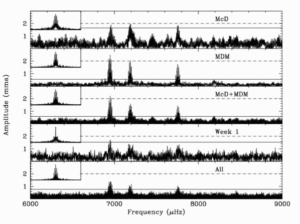
Figure 2: Temporal spectra of various subsets of PG 1618B data. Insets are the window functions. Solid (blue) horizontal line is the $4\sigma$ detection limit while the dashed (blue) lines are at 2 mma in all panels.

Our campaign was quite long (about 45 days) with a concentration of data at the beginning, but the best data (highest S/N and best conditions) were obtained at the end. We therefore grouped combinations of nightly runs into the subsets given in Table 2 for analysis. Table 2 also provides the temporal resolution (calculated as 1/$t_{\rm run}$ where $t_{\rm run}$ is the length of the observing run) and the $4\,\sigma$ detection limit (calculated using areas adjacent to the pulsation but outside of their window functions). The temporal spectra and window functions of these subsets are plotted in Fig. 2. A window function is a single sine wave of arbitrary, but constant amplitude sampled at the same times as the data. The central peak of the window is the input frequency, with other peaks indicating the aliasing pattern of the data. Each peak of the data spectrum intrinsic to the star will create such an aliasing pattern. As is evident from Fig. 2, the MDM data was significantly better than the rest, so we began our analysis with that subset.

Analysis of the MDM data was relatively easy and straightforward. In Fig. 3, the top panel shows the original FT, while the bottom panel shows the residuals after prewhitening by the frequencies indicated by arrows. The insets show the window function (top right) and an expanded view of a 65$\mu$Hz region around the close doublet. Frequencies, amplitudes and phases were determined by simultaneously fitting a nonlinear least-squares solution to the data. Since during the MDM observations the amplitudes were relatively constant, the solution proceeded as expected and prewhitening effectively removed the peaks and their aliases. The formal solution and errors for the MDM subset are given in Table 3.

Examination of the other data sets indicates that while PG 1618B was well-behaved during the MDM observations, it was not at other times. This was most noticeable in our examination the data collected during the first week. While the temporal spectrum has the cleanest window function, no peaks are detected above the $4\sigma$ detection limit (1.53 mma) even though peaks are detected in individual Lulin and McDonald runs (see Fig. 4 which will be discussed in §2.3). Combining the well-behaved MDM data with any other data set results in a decrease of amplitudes, indicating that outside of the MDM data, the amplitudes, phases, or even frequencies are not constant. If the pulsation properties were consistent throughout the campaign, data collected at smaller telescopes, with low S/N would still have been useful for reducing the overall noise. Unfortunately, such was not the case so all we can really conclude is that the MDM data detected all the pulsations that were occurring (above the detection limit) at that time while the pulsations intrinsic to PG 1618B must have been more complex at other times. It would be interesting to study the longer-term variability of PG 1618B, but using only 2 m-class telescopes.

Outside of the combined data sets, there are two frequencies that are detected above the $4\sigma$ detection limit during individual runs. The least-squares solutions for these frequencies are provided at the end of Table 3. The frequency at $\approx 9199\,\mu$Hz was above the noise only in the March 22 McDonald data, though a peak at the same frequency also appears in the Suhora data during March 16 and 21. The frequency at $\approx 8179\,\mu$Hz was above the noise only in the April 30 MDM data though corresponding peaks appear in the McDonald March 18, Lulin March 18, and Suhora March 21 runs. Since they are detected above the $4\sigma$ detection criteria for those runs, we include them in our discussion that follows.

2.3 Discussion

Silvotti et al. (2000) detected two frequencies in their discovery data while we clearly resolve four frequencies from our MDM dataset, and two more from individual data runs, bringing the total to six independent frequencies. We calculate the S00 resolution to be 5.5 $\mu$Hz and estimate their noise to be about 1 mma though this is misleading in that because of their short data runs, their window function effectively covers all of the remaining pulsations. However, for a strict comparison, we can say that our MDM data alone are $3\times$ better in resolution and have a detection limit twice as good, though in a practical sense our MDM data are far superior solely based on the duration of our individual data runs. Had S00 observed for longer durations (particularly with their CCD setup), their data would likely have been similar to the same number of runs from our MDM set. However, it is clearly safe to say that our MDM data alone are insufficient to describe the complexity of pulsations occurring within PG 1618B. As such, the remainder of our discussion which is based on the MDM data, can only be a minimum of what is really occurring.

2.3.1 Constraints on the pulsation modes

One of our goals is to observationally identify or constrain the pulsation modes of individual frequencies. Differing $m$ components of the same degree $\ell$ have degenerate frequencies unless perturbed, typically by rotation. If a star is rotating, then each degree will separate into a multiplet of $2\ell+1$ components with spacings nearly that of the rotation frequency of the star. As such, observations of multiplet structure can constrain the pulsation degree (for examples, see Winget et al. 1991 for pulsating white dwarfs and Reed et al. 2004 for sdB stars). For PG 1618B, there are no two frequency spacings that are similar, though there are not many frequencies to work with. The lack of observable multiplet structure is typical of sdBV stars but is likely limited to four possibilities: i) Rotation is sufficiently slow that all $m$ values remain degenerate within the frequency resolution of our data; ii) our line of sight is along the pulsation axis, with $\sin i\approx 0$, leaving only the $m=0$ mode observable because of geometric cancellation (Pesnell 1985; Reed, Brondel, & Kawaler 2005); iii) rapid internal rotation is such that $m$ multiplets are widely spaced and uneven (Kawaler & Hostler 2005); or iv) at most one pair is part of a multiplet with an unobserved component of the multiplet.

Spectroscopy can only rule out large splittings for possibility (i) as spectroscopic limits are typically $\approx 10$ km/s and from Fig. 1 of S00, PG 1618B appears as a “normal” sdB devoid of rapid rotation. Possibility (ii) can only be determined for cases in which the sdB star is part of a close binary such that the rotation and orbital axes can be inferred to be aligned. Since PG 1618 is only an optical double at wide separation, it does not constraint the alignment of the surface spherical harmonics. Similarly, possibility (iii) is virtually impossible to decipher unless the star pulsates in many (tens of) frequencies, and would still require some interrelation of spacings for modes of the same degree (Kawaler & Hostler 2005). Possibility (iv) also remains an option, though a difficult one to constrain. Higher resolution (and perhaps longer duration) spectroscopy would help to answer this question, and multicolor photometry or time-series spectroscopy might also be able to discern the spherical harmonics (see Koen 1998 and O’Toole et al. 2002 for examples of each).

Another quantity that can be used to constrain the pulsation modes is the frequency density. Using the assumptions that no two frequencies share the same $n$ and $\ell$ values (except possibly the close pair at $6946\,\mu$Hz), and that high-degree $\ell\geq 3$ modes are not observationally favored because of geometric cancellation (Charpinet et al. 2005; Reed, Brondel, & Kawaler 2005), we can ascertain whether the frequencies are too dense to be accounted for using only $\ell\leq 2$ modes. From stellar models, a general rule of thumb is to allow three frequencies per $1000\,\mu$Hz. We will ignore $f1$ which is too distant in frequency space and count $f5$ and $f6$ as a single degree $\ell$. This leaves four frequencies within 1235 $\mu$Hz; which can easily be accounted for using only $\ell\leq 2$ modes. Indeed, even if $f5$ and $f6$ do not share their $n$ and $\ell$ values, the frequency spectrum can still accommodate all of the detected frequencies without invoking higher degree modes. Of course this does not mean that they are not $\ell\geq 3$ modes, only that the pulsation spectrum is not sufficiently dense to require their postulation.

2.3.2 Amplitude and phase stability

If pulsating sdB stars are observed over an extended time period, it is common to detect amplitude variability in many, if not all, of the pulsation frequencies (eg. O’Toole et al. 2002; Reed et al. 2004; Zhou et al. 2006). Such variability can occasionally be ascribed to beating between pulsations too closely spaced to be resolved in any subset of the data. However, variations often appear in clearly resolved pulsation spectra where mode beating cannot be the cause. For PG 1618B, frequencies $f1$ and $f2$ are only detected during a single run each and frequencies $f5$ and $f6$ are too closely spaced to be resolved during individual runs, leaving only frequencies $f3$ and $f4$ available for analysis of amplitude variations.

Figure 4 shows the amplitude and phases of these two frequencies for individual data runs from McDonald and MDM observatories as well as a single Lulin run (marked by a triangle); these frequencies were not detected elsewhere. During the MDM observations, the amplitudes and phases for both frequencies are nearly constant (to within the errors) except for one low amplitude, but they have a significant variation in the McDonald and Lulin data. Of particular interest are the phases and amplitudes of $f4$, especially those during day three, in which we have both a McDonald and Lulin run that do not overlap in time. Between these two runs, the amplitude, which had been decreasing during the previous three days, suddenly increases to begin the same declining pattern again. The phases also show a bimodal structure early in the campaign with phases near $-0.20$ and $+0.25$ with the first phase jump occurring coincident with the amplitude increase. Except for the lack of sinusoidal amplitude variation, this has the appearance of unresolved pulsations. However, if the two unresolved frequencies had intrinsic amplitude variability, then it could reproduce the observations. However the MDM observations, which are not only steady, but have $f4$ phases intermediate to the McDonald and Lulin data, do not support this. Clearly, during the week of MDM observations, PG 1618B had neither amplitude nor phase variations and since the MDM phases do not coincide with phases from earlier in the campaign, unresolved pulsations are unlikely. Since the data obtained at MDM and McDonald observatories used the same acquisition system and time server (NTP), errors in timing also seem unlikely.

3 PG 0048+091

3.1 Observations

We originally observed PG 0048 as a secondary target during a campaign on KPD 2109+4401 (Zhou et al. 2006). Those data revealed a complex pulsation spectrum which we could not resolve with such limited sampling and a short time base. As such, PG 0048 was re-observed as a multisite campaign during Fall 2005. Five observatories participated in the campaign with the specifics of each run provided in Table 4. Though we were a bit unlucky with weather, over the course of our 16 night campaign we obtained 167.4 hours of data for a duty cycle of 44%. Details of the observing instruments and configurations are the same as for PG 1618B, except for the following: SAAO (1.9 m) used a frame transfer CCD with millisecond dead-times but only an $\approx 30\times 40$ arcsecond field of view, which resulted in no comparison stars within the CCD field. As such no transparency variations could be corrected and only photometric nights were used. Tubitak Observatory used a Fairchild CCD447 detector; during the first run the images had $1\times 1$ binning with a dead-time of 102 seconds, while subsequent runs used $2\times 2$ binning with a dead-time of 29 seconds. Bohyunsan Optical Astronomy Observatory (BOAO 1.9 m) data were obtained with a SiTe-424 CCD windowed to $580\times 445$ pixels, binned $2\times 2$ with an average dead time of 14 seconds. MDM and SAAO used red cut-off filters, making their responses very similar to blue-sensitive photoelectric observations, while Lulin, BOAO, and Tubitak used no filter making their sampling more to the red. As pulsations from sdB stars have little amplitude dependence in the visual and no phase dependence (Koen 1998; Zhou et al. 2006), mixing these data is not seen as a problem.

The standard procedures of image reduction, including bias subtraction, dark current and flat field correction, were followed using iraf. Differential magnitudes were extracted from the calibrated images using momf (Kjeldsen & Frandsen 1992), except for the SAAO data for which we used aperture photometry because there were no comparison stars. As described for PG 1618B, we again used low-order polynomials to remove airmass trends between our blue target star and the redder comparison stars. The lightcurves are normalized by their average flux and centered around zero, so the reported differential intensities are $\delta I=\left(I/\langle I\rangle\right)-1.$ Figure 5 shows the lightcurve of PG 0048 with each panel covering two days.

3.2 Analysis

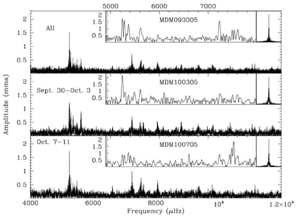
Figure 6: Comparison of temporal spectra for varying groups of PG 0048 data. The large panels show FTs for combinations of data (inclusive dates are labeled). The insets on the right are the window functions for the combinations of data to scale. The central insets are slightly enlarged FTs of individual runs obtained congruent with the larger panels and are labeled. They go from early to late within the campaign.

During the campaign, we completed a “quick-look” analysis of data runs as early as possible to ascertain the data quality and the pulsation characteristics of the star. We noticed early on that the temporal spectra of PG 0048 changed on a nightly basis with pulsation frequencies appearing and then disappearing on subsequent nights. Likewise, we knew that our analysis would be complicated by severe amplitude variations which would limit the usefulness of prewhitening techniques and could create aliasing. Figure 6 shows the effects of amplitude variations. The full panels are pulsation spectra for three groups of data: All of the data; data obtained from September 30 through October 3; and from October 7 through October 11. The right insets are the corresponding window functions plotted on the same horizontal scale. At such large scales, the windows appear as single peaks and show that the changes in the FTs are not caused by aliasing. The central insets are individual data runs within the larger set and show the variability between runs. When sets of data are combined in which the peak amplitudes are not constant, an FT will show the average amplitude. For the frequencies that appear in only a few runs, the amplitudes are effectively quashed in the combined FT. As PG 0048 is the most pulsation variable sdB star currently known, our immediate goal is to glean as many observables from these data as possible. While we do provide some interpretation, our aim is to provide sufficient information for theorists to test their models.

The complexity of the data meant it was necessary to analyze it using multiple techniques: We performed standard Fourier analyses on combined sets of observations to increase temporal resolution and lower the overall FT noise and analyzed individual runs of the best quality data. The analysis of individual runs represents a time-modified Fourier analysis, which is essentially a Gabór transform, except that we replace a Gaussian time discriminator with the natural beginnings and endings of the individual runs. As the best individual runs are not continuous with time (and nearly all are from MDM Observatory) the use of a Gaussian-damped traveling temporal wave discriminator (a standard Gabór transform) would not enhance the results. The temporal spectra of these runs are shown in Fig. 7. Runs mdm1005 and mdm1009, though long in duration, have gaps in them because of inclement weather, whereas the other 12 runs are gap-free. For these 12 runs aliasing in the FT is not a problem and the only constraints are the width of the peaks, which are determined by run length, and the noise of the FT, which is a combination of the signal-to-noise of each point and the number of data points within the run.

Frequencies, amplitudes and phases were determined using two different software packages, Period04 (Lenz & Breger 2004) and a custom (Whole Earth Telescope) set of non-linear least squares fitting and prewhitening routines. Each of the three data combinations in Fig. 6, the 12 gap-free data runs plotted in Fig. 7, the three data runs obtained during 2004, and the 10 runs from the discovery data (kindly provided by Chris Koen) were reduced using both software packages. Overall, more than 35 frequencies were fit during at least one data run. Table 5 provides information for 28 frequencies which have been detected above the $4\sigma$ detection limit. Column 1 lists a frequency designation; column 2 the frequency as fit to the highest temporal resolution data set in which each frequency is detected with the formal least-squares errors in column 3. Column 4 provides the standard deviation of the corresponding frequencies detected in individual runs and column 5 gives the number $N$ of individual runs in which that frequency was detected (from twelve 2005 runs and three 2004 runs). Tables 6 and 7 provide the corresponding amplitudes as fit for individual runs and various combinations of data acquired during the 2005 campaign, a re-analysis of the discovery data, and the 2004 MDM data. The last two rows of these tables provide the $4\sigma$ detection limits and temporal resolutions for the runs. Our determination that these frequencies are real and intrinsic to the star is based on i) detection by both fitting software packages, and amplitude(s) higher than the $4\sigma$ detection limit with ii) detection during several data runs, and/or iii) detection at amplitudes too large to be associated with aliasing.

3.3 Discussion

3.3.1 Frequency content

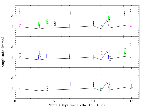
Figure 8: Amplitudes and errors of 12 frequencies detected in PG 0048. Each panel contains amplitudes for four frequencies (differentiated by point type and color) which may be shifted by $\pm 0.1$ day if they overlap. The solid line is the $4\sigma$ detection limit.

During our 2005 multisite campaign, we detected 24 pulsation frequencies from individual data runs plus an additional frequency from the combined data set (which was also detected in 2004). We recover all seven of the frequencies detected in the discovery data (K04), but only 14 of the 16 frequencies detected from our 2004 data. As can be seen from Table 5, PG 0048 shows an atypically large range of frequencies for sdBV-type pulsators, especially when considering that only one frequency, $f_{23}$ (11103.3 $\mu$Hz), can be identified as a linear combination (of $f_{6}$ and $f_{7}$). As noted in Table 5, only one frequency is detected in all of our data ($f_{2}$: $\sim$5244.9 $\mu$Hz) while the next most common frequency ($f_{13}$: $\sim$7237.0 $\mu$Hz) is detected in only 11 of the 15 runs. Several frequencies are only detected once or twice (e.g. $f_{12}$: $\sim$7154.3 $\mu$Hz), and so we should test if their amplitudes are sufficient to consider them to be real. If a particular frequency has amplitudes that are $1\sigma$ above the detection limit, then we might only expect to detect it 68% of the time. Figure 8 shows the amplitudes and $1\sigma$ errors for 12 different frequencies (four frequencies per panel) and the detection limit (solid line) for individual runs. The (black) circles in the top panel are for $f2$, which is detected in every run. However, the two frequencies indicated by (magenta) squares in the middle and bottom panels are only detected once, even though they are $>1\sigma$ above the detection limit. If their amplitudes were nearly constant (to within their errors), they would be detected at least 68% of the time. Another way to show this is in panel $a$ of Fig. 9 where the detections are plotted against their significance. We detect a total of 24 frequencies from 12 individual runs from our 2005 data. If we detected all 24 frequencies from every run, we would have made 288 detections, while we only actually made 75. The solid line shows the number of individual detections cumulative with significance (the number of standard deviations the detection was above the detection limit). In other words, 49 of our 75 detections were $2\sigma$ or less above the detection limit. The dashed line is the standard Gaussian probability distribution which shows that at $1\sigma$ significance, we should have made at least 196 (68%) detections. Since 64% of our detections are $\geq 1\sigma$, our 75 detections is well short of what we should have detected, indicating that the pulsation amplitudes are really falling below the detection limit. Panel $b$ compares the number of actual detections to the maximum pulsation amplitude. As expected, there is some correlation as the higher the amplitude, the easier it is to detect that frequency. Additionally, the highest amplitude (and therefore most easily detected) frequency is the same during 1997, 1998, and 2004 ($f8$: $\sim$5612.2 $\mu$Hz) but is only detected in $\sim 1/3$ of our 2005 data runs during which $f2$ ($\sim$5244.9 $\mu$Hz) had the highest amplitudes. This change in pulsation amplitudes will be further discussed in §3.3.3.

3.3.2 Constraints on mode identifications

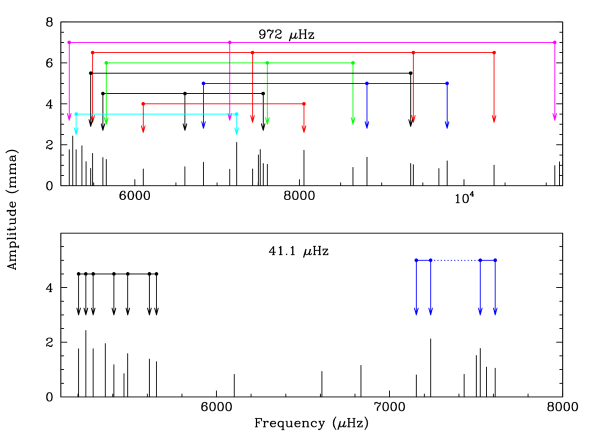
Figure 10: A schematic of the pulsation content of PG 0048 to indicate the nearly evenly spaced frequencies (provided in Table 8). The top panel shows the spacings that are integer multiples near $972~{}\mu$Hz and the bottom panel shows those near $41.1~{}\mu$Hz. For clarity, each set of multiplets are connected via horizontal bars at differing heights and have different colors (electronic version only, and black is used twice in the top panel).

As in §2.3.1, one of the best ways to relate pulsation frequencies to pulsation modes is via multiplet structure. With such a rich pulsation spectrum, it seems likely that some of the frequencies should be related by common frequency splittings. If not, then the pulsation spectrum is too dense (discussed below) for the frequencies to consist of only low-order $\ell\leq 2$ modes. There are two different spacings that occur many times with splittings near 972 and 41.1 $\mu$Hz. Table 8 lists these frequencies and the deviation from the average spacing between them, while Fig. 10 shows them graphically. While the spacings may be important, it is difficult to attach any physical meaning to them. A spacing of $972~{}\mu$Hz is far too large to be associated with stellar rotation, as it corresponds to a rotation period of only 17 minutes. There is currently no high-resolution spectrum of PG 0048, and the star’s main-sequence companion would complicate any attempts to measure its rotation velocity. However, the typical $v\sin i$ of sdBs is less than $\sim$ 5 km s^-1 (Heber, Reid, & Werner 2000). If we try to explain this large splitting using asymptotic theory (consecutive $n$ overtones rather than $m$ multiplets), we would expect successive overtones of the radial index to be roughly evenly spaced for large $n$, with one series for each $\ell$ degree. But the spacings observed in PG 0048 are irregular, requiring eight degrees (one for every line in Table 8), and $3\leq\ell\leq 7$ modes have reduced visibility because of geometric cancellation (Charpinet et al. 2005; Reed, Brondel, & Kawaler 2005). Theory suggests that sdBV stars should pulsate in low overtone modes and the spacings between successive low overtone modes should differ by several hundreds of $\mu$Hz (Charpinet et al. 2002), which again does not match what is observed.

Another asymptotic-like relation is the “Kawaler scheme” which has been recently presented by Kawaler et al. (2006) and Vuc̆ković et al. (2006). Though it is not compatible with the low overtone ($n$) pulsation theory associated with sdB pulsators, an improved frequency fit can sometimes be obtained using an asymptotic-like formula;

$$f(i,j)=f_{o}+i\times\delta+j\times\Delta$$

where $i$ has integer values, $j$ is limited to values of $-1,\,0,$ and $1$, $\delta$ is a large frequency spacing and $\Delta$ a small one. However, for the case of PG 0048, the small spacings are unrelated to the larger spacings and the larger spacings themselves do not interrelate, but rather appear in sets with differing spacings between the sets. So this scheme is not applicable for PG 0048.

The smaller, 41.1 $\mu$Hz spacings are more akin to what we would expect for rotationally split multiplets, though still large compared to typical measured rotation rates. If the low-frequency set are all components of a single multiplet, it would require very high degree ($\ell\geq 5$) pulsations, which are not observationally favored (Charpinet et al. 2005; Reed, Brondel, Kawaler 2005). The same is true for the high-frequency set if $f13$ and $f16$ belong to the same set. Since they are separated by $7\times 41.0\mu$Hz, it is certainly possible that $f12$-$f13$ and $f16$-$f18$ are just two pairs, but if they are all combined into a single multiplet, it would require $\ell\geq 5$ again. Yet these could also be just chance superpositions.

Since PG 0048 pulsates in so many frequencies, it is important to test the significance of the spacings discussed above. We did this by producing Monte Carlo simulations, randomly placing 28 frequencies within 6000 microHz of each other, and counting how often we could detect 14 frequency splittings the same to within about 5%. This criterion would find all but one of the splittings we actually observe. After analysing over one million simulations, we detected at least 14 splittings in nearly every case. In other words, the splittings we observe are not statstically significant.

Another tool we can use to place constraints on mode identifications is the mode density. As mentioned in §2.3.1, models predict roughly one overtone ($n$) per degree ($\ell$) per 1000 $\mu$Hz and though we have detected 28 frequencies, they are spread across nearly 6000 $\mu$Hz. Since we do not detect any multiplets that can be unambiguously associated with rotational splitting, it is likely the pulsations are degenerate in $m$. The average mode density is 4.8 frequencies per 1000 $\mu$Hz, which is too high to accommodate only $\ell\leq 2$, with degenerate $m$ modes and it gets worse as the frequencies are not quite distributed equally, but rather fall into loose groups, enhancing the density locally. The regions between 5200 and 6200 and 6600 to 7600 $\mu$Hz each contains 9 frequencies, and the region from 8800 to 9800 $\mu$Hz has 5 frequencies. If all $2\ell+1$ multiplets were filled (9 frequencies per 1000 $\mu$Hz), the frequency density would not require any $\ell\geq 3$ modes. However, as we do not detect appropriate multiplets within these frequency regions, the most likely result is that PG 0048 has too high a frequency density to exclude $\ell\geq 3$ modes using current models.

3.3.3 Amplitude and phase variability

Nearly all sdBV stars show some amount of amplitude variability. However, no other sdBV star has shown variability like that detected in PG 0048. An example of this is shown in Fig. 11, where the same 350 $\mu$Hz region is shown for the three data sets in Fig. 6. The bottom two panels are subsets of the top panel, which includes all of the data, and indicate how strikingly the pulsation spectrum changes with time.

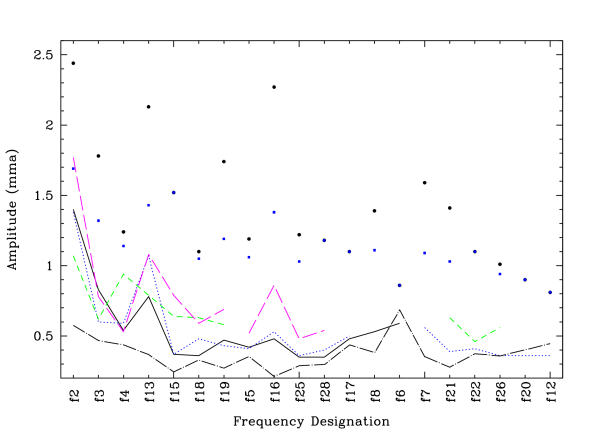
Figure 13: Amplitudes of frequencies detected in both individual runs and grouped data during 2005 for PG 0048. Dots (black) indicate the maximum amplitude, squares (blue) the average amplitude from individual runs. The lines indicate amplitudes from the following group datasets (from Table 6): dotted (blue) is G1, short-dashed (green) is G2, long-dashed (magenta) is G3, solid (black) is G4, and the dot-dashed (black) line is the $G4/A_{\rm max}$ ratio (or $G1/A_{\rm max}$ if no G4 value).

We can apply some constraints to the timescale of amplitude variability. Since pulsation frequencies can change amplitudes (even to the point of being undetectable) between individual runs, and in particular between runs from different observatories but for the same date, the next step was to divide up our longer data runs into halves. The FTs for six such runs are shown in Fig. 12 with each half containing about four hours of data. Particularly for runs mdm1007 (which can also be compared to saao1007) and mdm1010, the amplitudes change by factors of two over times as short as four hours. Low amplitude frequencies can easily become undetectable within that time. Figure 13 compares the maximum and average amplitudes detected in individual runs (the black circles and blue squares, respectively) to detections in groups of data (the lines) from Table 6. If the amplitudes were simply wandering around between values detected in individual runs, then the amplitude of the combined data would be an average of these values (the blue squares). However, since the combined amplitudes are significantly lower then the average amplitudes from individual runs, something else must be occurring to reduce the amplitudes.

Since changes in phase can impact pulsation amplitudes, we investigated that next. Figure 14 shows phases for eight of the most-often detected frequencies. $f2$ is the only frequency detected in every run, and we include the half-night analysis for it. For the other seven frequencies, we only determined phases for those runs in which they were detected above the $4\sigma$ limit. While Fig.14 indicates that most phases do not appear constant with time, most are within 20-30% of a central value.

To isolate and test the impact phase variation creates on data like ours, we analyzed simulated data with the following properties: The data are represented by a noise-free, single-frequency sine wave sampled corresponding to our 12 best individual runs with frequency $f2$. The amplitudes of each individual run are fixed at the measured values for $f2$ from Table 6 and we assume that no phase changes occur during an individual run. While the properties of $f2$ may not be the most representative of the variations detected, it is the only frequency detected every time, and so by using it, we sample the full range of amplitudes. If we used a different frequency, we could not know the actual pulsation amplitude during those runs without detections, and so would only be sampling the higher amplitude data points. We created simulations with the following phase properties: No change in phase, a fixed change of $\pm 10$% from the previous phase, a fixed change of $\pm 20$% from the previous phase, phases that are randomly set at the beginning of each run, and with the actual phase values for $f2$. The results of the simulations are given in Table 9 and the ratios are used in Fig. Follow-up observations of pulsating subdwarf B stars: Multisite campaigns on PG 1618+563B and PG 0048+091 where they are compared with our observations. The last line of Table 9 presents results with unique answers. As expected, there is a correlation between the amplitude and the amount of phase variation in that increasing changes in phase between individual runs decreases the measured amplitude of the data set as a whole. More useful are the ratios of the average amplitude to the average and maximum of the individual amplitudes ($\langle A\rangle/\langle A\rangle_{ind}$ and $\langle A\rangle/A_{max}$). These ratios can be compared with ratios from all frequencies, as has been done in Fig. Follow-up observations of pulsating subdwarf B stars: Multisite campaigns on PG 1618+563B and PG 0048+091. The shaded regions are the $1\sigma$ ratios produced from the phase simulations and the circles represent ratios with $G4$ data and the squares are for ratios using $G1$ data. The frequency ordering is the same as for Fig. 12, and like Fig. 12, the results indicate that for all but $f2$ and possibly $f6$, the amplitudes detected in groups of data are too low compared to individual amplitudes. Additionally, except for $f2$, the phases of Fig. 14 (and their standard deviations given in Table 10) are in discord with the amplitude ratios in that the amplitudes are too low. There does not seem to be sufficient phase variation to produce the low amplitudes of the group data. As such, it seems that more extreme circumstances are required. However, that leads into a more speculative area which we save for §3.3.4.

We conclude our observational portion of this paper with a summary provided in Table 10. In this table we have included all measurables (not in previous tables) discussed in this section and some that will be useful for the next section. Columns 2, 3, and 4 consider the number of expected detections based on the average significance of the actual detections; Columns 5 through 8 detail amplitudes detected for individual 2005 observing runs; Columns 9 through 12 provide ratios of individual to group amplitudes; and Column 13 lists the $1\sigma$ deviations of pulsation phases.

3.3.4 A possible cause of the amplitude/phase variability

Can we determine the cause of the erratic behaviour of PG 0048’s frequencies and amplitudes? We suggest that, with the possible exception of $f2$, the oscillations may be stochastically excited. While this is counter to current theory, supporting observations that we have in hand are 1) amplitudes that vary significantly between every individual run, and in less than $\sim$4 hrs; 2) the combined amplitudes are significantly lower than the average value indicating that phases are not coherent on these timescales; 3) the peaks in the FTs appear similar to those of known stochastic pulsators (compare Fig. 11 to Fig. 1 of Bedding et al. (2005) or Fig. 2 of Stello et al. (2006) for stochastic oscillators to those in, for example, Reed et al (2004) for “normal” sdB stars); and 4) the number of actual frequency detections compared to the expected number based on significance (the ratio of the two lines in the left panel of Fig. 9). We note that this is not conclusive evidence, but is suggestive and so we will pursue a stochastic nature for PG 0048’s pulsations in the remainder of this section.

Recently, Stello et al. (2006) found that short mode lifetimes in red giants can severely limit the possibility of measuring reliable frequencies. The difficulty arises because the frequencies can disappear entirely and when they are re-excited (even if this occurs prior to complete damping), they do not maintain the same phase. The parallel with our analysis of PG 0048 are clear and this kind of variability has been seen before in sdBVs. In a study of KPD 2109+4401, Zhou et al. (2006) found substantial variation in the amplitudes of two modes during their 32 night campaign. A brief analysis found that at least one of these modes, and possibly both of them, satisfied the criterion outlined by Christensen-Dalsgaard et al. (2001; hereafter JCD01) for stochastically excited pulsations, rather than overstable driving. The criterion compares the ratio of amplitude scatter to the mean amplitude; for stochastic pulsations, this ratio should be $\approx 0.52$. Stochastic processes in pulsating sdB stars have also been discussed by Pereira & Lopes (2005) in the context of the complex sdB pulsator PG 1605+072, which is known to have variable amplitudes (O’Toole et al. 2002; Reed et al. 2007, in press). Using the JCD01 criterion, Pereira & Lopes deduced that none of the modes of that star were consistent with stochastic excitation. However, O’Toole et al. (2002) noted amplitude changes between years, while Pereira & Lopes (2005) only studied 7 nights of data, and as such their analysis was likely affected by the short length of their time series.

A limitation to the JCD01 test is that the damping times of the oscillations should be longer than the timescale used for determining the amplitudes. Our analysis of $\sim 4$ hour segments of PG 0048 data indicate that amplitude variations are on very short timescales that are shorter than the observing time for individual runs (see Figs. 7 and 12). We provide the JCD01 parameter values $\sigma_{A}/\langle A\rangle$ in Column 7 of Table 10, but we suggest that the JCD01 test is not appropriate for PG 0048. Aside from the JCD01 test, we can attempt to reproduce some of the observational properties using simple simulations with damped and randomly re-excited frequencies. The complexity of the actual data is such that we cannot hope to reproduce it directly, but instead will strive to fit the observations listed at the beginning of this section. Our simulations follow the simple prescription (equations 2 and 3) of Chaplin et al. (1997) summarized as follows: The pulsations themselves are described by sine waves of the form $A(t)=A\cos((2\pi\cdot f)(t-\phi))$, with the amplitude modified in two ways; it is damped exponentially as $A=A_{o}\exp(-t_{e}/t_{d})$ where $A_{o}$ is the maximum amplitude, $t_{e}$ is the time since the last excitation and $t_{d}$ is the damping timescale. The pulsation is re-excited by setting $t_{e}=0$ when time $t$ exceeds an excitation timescale ($t_{exc}$). The time before the first re-excitation is randomly set to some fraction of the excitation timescale and every time the pulsation is re-excited, the phase is randomly set and the excitation timescale and pulsation amplitude can vary randomly by up to 20% or their original values. The free parameters of the simulation are the input amplitude, which is the maximum amplitude attainable and the excitation and damping timescales ($A_{o}\,,t_{exc}\,$ and $t_{d}$, respectively). The simulation includes frequencies, amplitudes, and phases for up to 100 pulsations with an unlimited number of data runs (input as run start time, the number of data points, and cycle time). We will concentrate on matching the MDM runs in Table 6. This is the $G1$ data set with an average run length of 9.35 hours ($\sim 0.4d$), containing $\sim 2800$ data points each, an average detection limit of 0.88 mma, and average ratios $A_{\rm G1}/\langle A\rangle=0.44\pm 0.14$ and $A_{\rm G1}/A_{\rm max}=0.37\pm 0.09$.

To match the observational constraint that the pulsation amplitude can reduce by half in a four hour span, the damping timescale is necessarily less than 5.8 hours. With this constraint, we produced a grid of simulations with $1\leq t_{d}\leq 7$ hours in 1 hour increments and $1\leq t_{exc}\leq 33$ hours in 2 hour increments. Qualitatively, if no re-excitations occur during an individual run, the FT is single-peaked whereas multiple re-excitations create a variety of complex, multi-peaked FTs, depending on how similar the randomized phases were (the less alike the phases for each re-excitation, the lower the overall amplitude and more and similar-amplitude peaks appear in the FT). For small $t_{exc}$, the FT becomes increasingly complex with most simulations resulting in many low-amplitude peaks distributed across a couple hundred $\mu$Hz. However, such complex patterns are not consistent with observations and so we discount small values for $t_{exc}$. Amplitudes in the FT are reduced with large values of $t_{exc}$ and small values of $t_{d}$ while the scatter increases with increasing values for both. An increase in amplitude scatter is necessary to produce the low rate of detections.

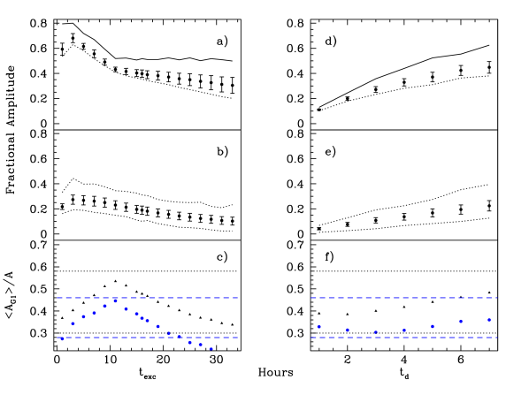
Figure 16: Simulations of randomly excited and damped pulsations. Panels a, b, and c show the effect of changing the excitation timescale for a fixed damping timescale of $t_{d}=5$ hours. Panel a and b show the results of simulating a single 9.35 hour run and the nine MDM runs in Table 2, respectively. The points indicate the average amplitude with $1\sigma$ error bars, the solid line is the maximum amplitude from an individual simulation and the dotted line indicated the minimum amplitude detected from an individual simulation. Panel c shows the ratios $\langle A_{G1}\rangle/A_{max}$ (blue circles) and $\langle A_{G1}\rangle/\langle A_{ind}\rangle$ (black triangles). The dashed blue (dotted black) lines indicate the observed range in PG 0048 for $\langle A_{G1}\rangle/A_{max}$ ($\langle A_{G1}\rangle/\langle A_{ind}\rangle$). Panels d, e, and f correspond to panels a, b, and c except that the excitation timescale is fixed at $t_{exc}=19$ hours and the damping timescale is varied.

As we now have all the pieces in place, we can ask how well the simulations reproduce the observational constraints we set at the beginning of this section. A selection of the results are shown in Figs. 16 and Follow-up observations of pulsating subdwarf B stars: Multisite campaigns on PG 1618+563B and PG 0048+091. Panels a, b, and c of Fig. 16 have $t_{d}$ fixed at 5 hours and vary $t_{exc}$ whereas panels d, e, and f fix $t_{exc}$ at 19 hours and vary $t_{d}$. Panels a and d are the results for individual runs and panels b and e are for the combined nine-run data set. The points represent the average ($\langle A\rangle$) with $1\sigma$ deviations while the lines indicate maximum ($A_{max}$) and minimum amplitudes. Panels c and f show the ratios $\langle A_{G1}\rangle/A_{max}$ and $\langle A_{G1}\rangle/\langle A_{ind}\rangle$; the average amplitude from the combined data divided by the maximum or average amplitude from the individual runs. Figure Follow-up observations of pulsating subdwarf B stars: Multisite campaigns on PG 1618+563B and PG 0048+091 shows the expected rate of detections calculated in the following manner: The detection limit was calculated using the observed ratios $\langle A_{max}\rangle/0.88=1.56$ and $\langle A\rangle/0.88=1.32$ for the MDM data with an average detection limit of 0.88 mma and solving for the new detection limit. The dotted line is the observed detection rate of 26% and it is interesting that none of simulations are that low if using the average detected amplitude. While the overall amplitudes can become quite small, the average follows that, which is used to calculate our detection limit in the top panel. However, most values of $t_{d}$ matched the observed rate near $t_{exc}=19$-$21$ hours using $A_{max}$. The simulations that best fit the observational constraints are those which have $4\leq t_{d}\leq 6$ hrs and $13\leq t_{exc}\leq 21$ hrs. The lower values of $t_{exc}$ better fit the $\langle A_{G1}\rangle/A$ ratios while the larger values are a better match for the detection rate. These relatively simple simulations are able to fit all of the observed constraints, thus explaining the amplitude variations, their lower detection limits in groups of data, the relatively low detection rate and the appearance of the peaks in the FT. What they cannot explain however, is the relative lack of phase variability in some frequencies (though relatively few were measurable) and why stochastic processes should occur in the first place.

Stochastic oscillations are usually presumed to be driven by random excitations caused by convection (see Christensen-Dalsgaard 2004 for a review concerning the Sun). The He II/He III convection zone in sdB stars was investigated by Charpinet et al. (1996), who determined that it could not drive pulsations. However, it appears that they did not investigate this zone for convective motions but rather as a driver for the $\kappa$ mechanism. So some ambiguity remains here. There is also convection or semi-convection in the cores of sdB stars, and it is possible that the eigenfunctions could be sampling this region. Whatever the case, the extreme amplitude and phase variability of PG 0048 poses a significant challenge to the iron driving mechanism found by Charpinet et al. (2001) to excite pulsations in sdB stars. Though it is beyond the scope of this paper to ascertain the cause of the random amplitude variations, we find that the observed properties are consistent with our simplified randomly excited simulations and that the amplitude spectrum resembles those of pulsators that are stochastically driven.

4 Conclusions and Future Work

We have carried out multisite campaigns for two sdB pulsators, PG 1618+563B and PG 0048+091 and in both cases, our observations were superior to the published discovery data, yet questions concerning these two stars still remain. Our MDM observations of PG 1618B (obtained under good conditions) show characteristics typical of about half the objects in the sdBV (V361 Hya) class: A small number of stable (in amplitude) frequencies with a closely spaced pair. In contrast, the data obtained at McDonald observatory – under non-photometric conditions – show PG 1618B to be a complex pulsator with four “regions” of power showing amplitude and phase variability. An ensemble analysis of any combinations of data other than the MDM set are hindered by poor least-squares fitting and amplitudes reduced below detectability. Such poor fitting can be caused by unresolved frequencies with intrinsic amplitude variability (O’Toole et al. 2002) or randomly excited pulsations (Christensen-Dalsgaard 2004). So despite having expended considerable effort to obtain not only multisite, but extended time-base observations, we were only reasonably successful at detecting pulsations from our 2 m telescope data; and these show the star to be two-faced. With this dichotomy of observational results, PG 1618B remains an interesting target for more follow-up observations; particularly to examine its long-term frequency stability.

PG 0048 is much more complex than PG 1618B, yet it too has shown somewhat stable pulsation amplitudes at one epoch (the discovery and 2004 data) and wildly variable amplitudes at another (2005). Though an extremely rich pulsator with at least 28 independent frequencies, many modes are only excited to amplitudes above the noise occasionally, often for very short lengths of time. These behaviors are consistent with stochastic pulsations and we have performed several tests along these lines. We simulated damped and re-excited pulsations and found that the observations were best matched with damping timescales between 4 and 6 hours and excitation timescales between 13 and 19 hours. We detected common frequency splittings of 972 and 41 $\mu$Hz which may be related to multiplet structure, but could reproduce these using Monte Carlo splittings of random spacings. So while they may be intrinsic to the pulsation of PG 0048, we cannot be sure. We can be sure that PG 0048’s rich pulsation spectrum is too dense to be accounted for using only $\ell\leq 2$ modes regardless of how many $m$ components are present.

The observations presented in this paper provide some very interesting and confusing results. Pulsations that appear stable during some times and variable at others; attributes that have also been observed in other sdBV stars as well (KPD 2109+2752, PG 1605+072, and HS 1824+5745, just to name a few). The pulsations in PG 0048 present observables that seem best described by randomly excited oscillations which would be in contrast to the proposed driving mechanism (Charpinet et al. 2001). If validated, it would represent a new direction in sdB pulsations (and modeling too!). However, a longer time series may be the only way to clarify the nature of the oscillations in this star. Ideally this would take place on at least 2 m-class telescopes and cover several weeks.

Table 1: Observation record for PG 1618B. The first two runs were obtained in 2003, while the rest were obtained in 2004.

Run	Date	Start	Length	Int.	Observatory
	UT	hr:min:sec	(Hrs)	(s)
suh16mar	17 Mar	00:07:58	3.3	10	Suhora 0.6 m
lul031705	17 Mar	16:46:33	5.6	10	Lulin 1.0 m
McD031805	18 Mar	04:34:00	1.1	5	McDonald 2.1 m
lul031805	18 Mar	15:14:24	6.1	10	Lulin 1.0 m
McD031905	19 Mar	08:40:40	3.1	5	McDonald 2.1 m
lul031905	19 Mar	19:58:41	1.3	15	Lulin 1.0 m
baker032005	20 Mar	04:29:30	5.6	25	Baker 0.4 m
McD032005	20 Mar	06:35:00	5.8	5	McDonald 2.1 m
lul032005	20 Mar	15:17:19	6.0	10	Lulin 1.0 m
suh20mar	20 Mar	18:59:00	8.3	10	Suhora 0.6 m
lul032105	21 Mar	16:44:59	0.7	15	Lulin 1.0 m
suh21mar	21 Mar	18:20:20	8.6	20	Suhora 0.6 m
McD032205	22 Mar	04:33:00	7.8	5	McDonald 2.1 m
suh22mar	22 Mar	18:40:40	2.2	20	Suhora 0.6 m
McD032305	23 Mar	04:12:10	8.0	5	McDonald 2.1 m
mdr299	29 Mar	04:11:15	4.7	15	Baker 0.4 m
mdr301	31 Mar	04:28:10	7.0	15	Baker 0.4 m
mdr302	02 Apr	02:53:10	8.1	10	Baker 0.4 m
bak040305	03 Apr	03:20:46	7.9	15	Baker 0.4 m
bak040405	04 Apr	04:23:10	5.6	15	Baker 0.4 m
bak040505	05 Apr	03:17:10	6.6	10	Baker 0.4 m
bak041405	14 Apr	03:45:00	7.1	10	Baker 0.4 m
bak041505	15 Apr	02:26:30	8.4	10	Baker 0.4 m
bak041605	16 Apr	02:50:30	7.9	10	Baker 0.4 m
bak041705	17 Apr	03:18:50	5.3	15	Baker 0.4 m
bak041805	18 Apr	02:56:00	7.7	15	Baker 0.4 m
mdm042605	26 Apr	04:25:30	7.3	5	MDM 2.4 m
mdm042705	27 Apr	04:16:50	7.6	5	MDM 2.4 m
mdm042805	28 Apr	04:14:00	7.8	3	MDM 2.4 m
mdm042905	29 Apr	04:18:00	1.6	5	MDM 2.4 m
mdm043005	30 Apr	04:04:30	7.8	3	MDM 2.4 m
mdm050105	01 May	04:05:30	7.8	5	MDM 2.4 m
mdm050205	02 May	03:36:40	5.3	5	MDM 2.4 m

Table 2: Subsets of data for PG 1618B. For column 2, observatories are 1) McDonald Observatory; 2) Suhora Observatory; 3) Lulin Observatory; 4) Baker Observatory; and 5) MDM Observatory.

Set	Observatory(ies)	Inclusive Dates	Resolution	$4\sigma$ detection limit
			$\mu$Hz	mma
McD	1	18 - 23 March	2.2	1.64
MDM	5	26 Apr - 02 May	1.9	0.55
McD+MDM	1, 5	18 - 02 May	0.3	0.59
Week 1	1, 2, 3	17 - 23 March	1.5	1.53
All	1, 2, 3, 4, 5	17 - 02 May	0.2	0.77

Table 3: Our least-squares fit solution for the pulsation periods, frequencies, and amplitudes detected in PG 1618B. Formal least-squares errors are given in parentheses. Frequencies marked with a dagger (^†) were only detected during individual runs (one each) while the remaining frequencies are from the MDM data set.

Des.	Period	Frequency	Amplitude
	(s)	($\mu$Hz)	(mma)
$f1^{\dagger}$	108.7092 (0.0518)	9198.85 (4.38)	1.79 (0.39)
$f2^{\dagger}$	122.2574 (0.0597)	8179.46 (4.00)	1.04 (0.21)
$f3$	128.9549 (0.0008)	7754.64 (0.05)	1.71 (0.09)
$f4$	139.0571 (0.0008)	7191.28 (0.04)	2.04 (0.09)
$f5$	143.9290 (0.0011)	6947.87 (0.05)	2.22 (0.10)
$f6$	143.9759 (0.0014)	6945.60 (0.07)	1.64 (0.10)

Table 4: Observations of PG 0048

Run	Date	Start	Length	Int.	Observatory
	UT	hr:min:sec	(Hrs)	(s)
2004
mdr285	10 Oct	04:21:00	6.2	15	MDM 1.3 m
mdr290	12 Oct	03:39:00	7.3	15	MDM 1.3 m
mdr295	14 Oct	03:34:00	7.4	15	MDM 1.3 m
2005
boao	26 Sept.	10:30:20	5.0	10	BOAO 1.9 m
mdm092805	28 Sep	07:32:30	4.5	15	MDM 1.3 m
mdm092905	29 Sep	02:53:00	9.5	15	MDM 1.3 m
mdm093005	30 Sep	02:44:00	9.5	15	MDM 1.3 m
turkSep3sdb	30 Sep	17:37:54	9.3	10	Tubitak 1.5 m
mdm100105	01 Oct	02:46:00	9.4	10	MDM 1.3 m
turk1Octsdb	01 Oct	21:26:58	4.1	10	Tubitak 1.5 m
mdm100205	02 Oct	09:57:30	2.3	15	MDM 1.3 m
turk2Octsdb	02 Oct	20:51:36	4.8	10	Tubitak 1.5 m
mdm100305	03 Oct	02:32:00	9.1	10	MDM 1.3 m
turk3Octsdb	03 Oct	17:41:49	8.5	10	Tubitak 1.5 m
mdm100405	04 Oct	09:24:00	2.2	15	MDM 1.3 m
mdm100505	05 Oct	02:33:00	9.4	12	MDM 1.3 m
mdm100605	06 Oct	02:23:00	9.4	10	MDM 1.3 m
mdm100705	07 Oct	02:15:00	9.6	12	MDM 1.3 m
lul7Oct	07 Oct	18:32:20	1.6	20	Lulin 1.0 m
a024	07 Oct	20:28:14	6.2	10	SAAO 1.9 m
mdm100805	08 Oct	03:17:00	8.5	15	MDM 1.3 m
a039	08 Oct	21:31:48	5.4	10	SAAO 1.9 m
mdm100905	09 Oct	02:17:00	9.3	10	MDM 1.3 m
a057	09 Oct	20:11:53	4.1	10	SAAO 1.9 m
mdm101005	10 Oct	02:06:00	9.6	10	MDM 1.3 m
a077	10 Oct	19:58:49	6.5	10	SAAO 1.9 m
mdm101105	11 Oct	02:00:00	9.6	10	MDM 1.3 m

Table 5: Frequencies detected for differing subsets of PG 0048 data. Column 1 is the frequency designation; column 2 is the frequency determined from a combined data set; column 3 is the formal least-squares error from the combined data set; column 4 is the standard deviation of frequencies detected from individual runs; and column 5 is the number of individual 2005 and 2004 runs in which that frequency is detected. All frequencies are given in $\mu$Hz. (^† indicates frequencies that were not detected in 2005.)

Des.	Freq.	$\sigma_{fit}$	$\sigma$	$N$
$f1$	5203.1	-	5.9	2
$f2$	5244.9	0.16	4.6	15
$f3$	5287.6	0.03	3.6	8
$f4$	5356.9	0.05	9.8	8
$f5$	5407.0	0.07	3.2	1
$f6$	5465.1	-	-	1
$f7$	5487.2	0.05	8.5	7
$f8$	5612.2	0.05	4.5	8
$f9$	5652.9	-	-	$1^{\dagger}$
$f10$	6609.2	-	9.0	2
$f11$	6834.3	0.15	9.0	$3^{\dagger}$
$f12$	7154.3	0.08	1.4	1
$f13$	7237.0	0.04	7.0	10
$f14$	7430.1	-	-	1
$f15$	7501.3	0.07	-	1
$f16$	7523.9	0.06	15.0	8
$f17$	7560.0	-	-	1
$f18$	7610.1	0.07	5.6	5
$f19$	8055.5	0.06	10.1	8
$f20$	8651.4	0.08	-	1
$f21$	8820.6	0.08	6.4	4
$f22$	9352.8	0.07	16.3	1
$f23$	9385.3	0.28	8.9	$1^{\dagger}$
$f24$	9694.6	-	-	1
$f25$	9795.1	0.08	18.8	2
$f26$	10366.8	0.08	1.4	2
$f27$	11103.3	-	-	$1^{\dagger}$
$f28$	11159.8	0.07	-	1

Table 6: Amplitudes detected for differing subsets of PG 0048 data during the 2005 multisite campaign. The last two rows give the $4\sigma$ detection limit and the temporal resolution for each subset. Note that all frequencies are given in $\mu$Hz. Runs 1 through 12 are boao, mdm0929, mdm9030, mdm1001, mdm1003, mdm1006, mdm1007, saao1007, mdm1008, mdm1010, saao1010, and mdm1011 and runs G1 through G4 are MDM only, Oct. 1 - 3, Oct. 7 - 11, and all the 2005 data, respectively.

Des.	1	2	3	4	5	6	7	8	9	10	11	12	G1	G2	G3	G4
$f1$						1.11		1.69
$f2$	2.44	1.03	1.48	1.25	2.26	1.12	0.93	2.34	1.70	2.19	2.42	1.77	1.38	1.07	1.77	1.40
$f3$		1.21	1.39	1.22	1.01	1.26			1.77				0.60	0.62	0.78	0.83
$f4$	1.13		1.30	1.24			1.07				1.01		0.59	0.94	0.53	0.54
$f5$				1.19									0.41		0.52	0.42
$f6$		0.86														0.59
$f7$	1.06	1.05			1.02				0.87	1.59			0.56		0.66
$f8$		0.98	1.12	1.39	1.06				1.02					0.92		0.53
$f10$							0.94
$f12$		0.81											0.36
$f13$		1.36				1.04	0.95	1.68	1.50	1.46	2.13		1.07	0.79	1.08	0.78
$f14$							0.83
$f15$							1.52						0.37	0.64	0.79	0.37
$f16$			0.97			1.36	2.26		1.39		1.78	1.09	0.53		0.86	0.48
$f17$											1.10		0.50			0.48
$f18$			1.00			1.09	1.10					0.99	0.48	0.63	0.59	0.36
$f19$	1.12	0.89	1.08								1.13	1.74	0.43	0.58	0.69	0.47
$f20$									0.90				0.36		0.44
$f21$					1.41		0.81		0.94				0.39	0.63
$f22$				1.10									0.41	0.46
$f23$															0.44
$f24$				0.85
$f25$				1.22			0.88						0.36		0.48	0.35
$f26$					0.91		1.01						0.36	0.56
$f28$												1.18	0.40		0.54	0.35
$4\sigma$	0.96	0.75	0.84	0.85	0.90	1.02	0.76	1.60	0.84	1.07	1.00	0.91	0.31	0.47	0.43	0.28
$1/T$	53	29	29	31	29	29	29	46	31	29	39	36	0.9	2.2	2.2	0.8

Table 7: The same as Table 6 for the discovery data (1997 and 1998; courtesy of C. Koen) and 2004 MDM data. Runs dd1 through dd10 are tex151, tex157, tex177, tex182, tex186, dmk157, dmk163, ck261, ck263, and ck265, runs 1 through 3 are mdr285, mdr290, and mdr295, and runs G1 through G4 are all 1997, October 1998, November 1998, and 2004 data, respectively.

Des.	dd1	dd2	dd3	dd4	dd5	dd6	dd7	dd8	dd9	dd10	1	2	3	G1	G2	G3	G4
$f1$										2.63
$f2$					3.18						1.11	1.95	2.01	2.78			1.65
$f3$	5.86		3.52				2.77				1.76	4.29			2.10		1.54
$f4$			3.39	2.33						3.40	1.96	1.14	1.90	1.93	1.34		1.57
$f5$					1.96												0.55
$f7$			1.96	1.20	2.12						0.93	0.84		1.94		2.16	0.75
$f8$	4.94*	5.80	3.97	4.39	3.10	3.43	3.57	3.95	4.96		2.85	3.10	3.14	4.05	3.34	2.01	2.97
$f9$													1.28				0.65
$f10$													1.18				0.68
$f11$											1.03	1.16	0.98		1.56		1.00
$f13$											2.76	1.55	1.56				1.56
$f16$	4.31*											2.28	1.22				1.26
$f17$			1.55	2.17			1.69							1.40	1.56
$f18$											1.25						0.77
$f19$					2.36				3.29		1.21	1.08	2.03	1.17		1.99	1.06
$f20$				1.75
$f21$												0.93					0.74
$f22$				2.43										1.26
$f23$												1.04					0.65
$f24$																	0.53
$f27$												1.00
$4\sigma$	5.38	3.54	1.50	1.20	1.70	2.06	1.63	3.80	3.17	2.44	0.75	0.82	0.97	1.14	1.21	1.97	0.50
$1/T$	194	132	69	96	84	96	84	174	185	111	41	38	37	0.8	5.4		0.9

Table 8: PG 0048 pulsation frequencies split by integer multiples near 972 and 41.1 $\mu$Hz. The first column gives the minimum degree $\ell$ for the multiplet and the order for each row is from the top of Table 5, or in descending frequencies and the number in parentheses indicates the integer multiple between itself and the previously listed frequency and the percent deviation from 972 or 41.1 $\mu$Hz.

$\ell_{min}$	Des.	Designations for related frequencies
Spacings of 972 $\mu$Hz
3	$f1$	$f12$ (2, 0.2%); $f27$ (4, 1.4%)
3	$f7$	$f14$ (2, 0.2%); $f23$ (2, 0.4%); $f26$ (1, 0.8%)
1	$f8$	$f10$ (1, 2.4%); $f17$ (1, 2.4%)
2	$f9$	$f18$(2, 0.5%); $f20$ (1, 6.9%)
2	$f11$	$f21$ (2, 2.0%); $f25$ (1, 0.07%)
1	$f3$	$f13$ (2, 0.4%)
2	$f6$	$f22$ (4, 0.2%)
Spacings of 41.1 $\mu$Hz
6	$f1$	$f2$ (1, 1.7%); $f3$ (1, 3.9%); $f5$ (3, 3.2%); $f7$ (2, 2.4%); $f8$ (3, 1.5%); $f9$ (1, 0.1%)
6 (1, 1)	$f12$	$f13$ (2, 0.05%); $f16^{\dagger}$ (7, 0.02%); $f18$ (2, 5.9%)

Table 9: Results of simulations for phase changes using $f2$ as the template and a comparison with observations. Column 1 indicates how the phase was changed in the simulation and columns 2 and 3 provide the average amplitude and standard deviation of $>100,000$ simulations. Columns 4 and 5 provide ratios comparing amplitudes between individual runs and that of the combined simulated data set. The bottom row provides the average amplitude from the individual runs and results from the simulations with constant phase and fixed amplitudes and phases with those observed for $f2$.

Sim	$\langle A\rangle$	$\sigma$	$\langle A\rangle/\langle A\rangle_{ind}$	$\langle A\rangle/A_{max}$
10%	1.50	0.03	0.97	0.66
20%	1.35	0.10	0.88	0.60
Random	1.06	0.11	0.69	0.47
$\langle A\rangle_{ind}$	constant phase		$A_{obs}$ & $\phi_{obs}$
1.54	1.55		1.49

Table 10: Observed properties of individual frequencies.

Des.	#det	$\langle\sigma_{d}\rangle$	#exp	$\langle A\rangle$	$\sigma_{A}$	$\sigma_{A}/\langle A\rangle$	$A_{max}$	$A_{G4}/\langle A\rangle$	$A_{G4}/A_{max}$	$A_{G1}/\langle A\rangle$	$A_{G1}/A_{max}$	$\sigma_{\phi}$ (%)
$f1$	2	0.38	3	1.30	0.41	0.32	1.69	-	-	-	-	-
$f2$	12	3.69	12	1.69	0.53	0.31	2.44	0.83	0.57	0.82	0.57	9.6
$f3$	5	2.63	11	1.32	0.22	0.17	1.77	0.63	0.47	0.45	0.34	-
$f4$	5	1.59	10	1.14	0.15	0.13	1.30	0.47	0.44	0.52	0.48	8.4
$f5$	2	0.92	7	1.06	0.19	0.18	1.19	0.40	0.35	0.39	0.34	-
$f6$	1	0.11	1	0.86	-	-	0.86	0.67	0.67	-	-	-
$f7$	5	1.16	8	1.09	0.19	0.17	1.59	-	-	0.51	0.35	7.9
$f8$	5	1.50	10	1.11	0.09	0.08	1.39	0.48	0.38	-	-	6.3
$f9$	1	-	-	-	-	-	-	-	-	-	-	-
$f10$	1	1.06	8	0.94	-	-	0.94	-	-	-	-	-
$f11$	1	-	-	-	-	-	-	-	-	-	-	-
$f12$	1	0.33	3	0.81	-	-	0.81	-	-	0.44	0.44	-
$f13$	7	2.32	11	1.43	0.36	0.25	2.13	0.55	0.37	0.75	0.50	15.8
$f14$	1	0.41	3	0.83	-	-	0.83	-	-	-	-	-
$f15$	1	2.75	11	1.52	-	-	1.52	0.24	0.24	0.24	0.24	-
$f16$	6	2.60	11	1.38	0.44	0.32	2.26	0.35	0.21	0.38	0.23	15.0
$f17$	1	0.50	4	1.10	-	-	1.10	0.44	0.44	0.45	0.45	-
$f18$	4	0.94	7	1.05	0.18	0.17	1.10	0.43	0.33	0.46	0.44	25.9
$f19$	5	1.79	10	1.19	0.26	0.22	1.74	0.39	0.27	0.36	0.25	7.3
$f20$	1	0.32	2	0.90	-	-	0.90	-	-	0.40	0.40	-
$f21$	3	1.16	8	1.03	0.26	0.25	1.41	-	-	0.38	0.28	-
$f22$	1	1.32	9	1.10	-	-	1.10	-	-	0.37	0.37	-
$f23$	1	-	-	-	-	-	-	-	-	-	-	-
$f24$	1	0.00	1	-	-	-	-	-	-	-	-	-
$f25$	2	2.25	11	1.03	0.24	0.23	1.22	0.34	0.29	0.35	0.30	-
$f26$	3	0.76	6	0.94	0.17	0.18	1.01	-	-	0.41	0.36	-
$f27$	1	-	-	-	-	-	-	-	-	-	-	-
$f28$	1	1.42	9	1.18	-	-	1.18	0.30	0.30	0.34	0.34	-

Figure 1: Lightcurves for PG 1618B data. The top four panels show the coverage during the multisite portion of the campaign from March 17 – 24, 2005, while the bottom panel shows an enlarged section of a run obtained at MDM. Note that the scales are different for the bottom panel. The line indicates our fit to the data.

Figure 3: Temporal spectrum of PG 1618B data. Top panel shows the original FT of the combined MDM data while the bottom panel shows the residuals after prewhitening. Prewhitened frequencies are indicated by arrows. Insets show an enlarged view of the frequency doublet and the window function.

Figure 4: Amplitudes and phases of the two frequencies in PG 1618B that are resolvable nightly. The data are only those from McDonald and MDM observatories except for a single Lulin run (marked by a triangle). The dashed lines indicate our fits to the MDM data. Note that the time axis is discontinuous.

Figure 5: Lightcurves for the PG 0048 data. Each panel is two days.

Figure 7: Temporal spectra for individual PG 0048 observing runs.

Figure 9: a) The number of detections of frequencies from individual runs for PG 0048 compared to Gaussian probability. The number of possible detections (dashed line) compared to the amount of actual detections (solid line) depending on the detection significance. b) A comparison between the number of detections for individual frequencies and the maximum amplitude detected.

Figure 11: A 350 $\mu$Hz region of PG 0048’s FT covering three modes at $\sim$7497.4 $\mu$Hz, $\sim$7524.1 $\mu$Hz and $\sim$7605.9 $\mu$Hz. The panels correspond to those in Fig. 6. The spectral windows at the top of each panel cover the same frequency range as the observations, to give the reader an appreciation of how dense these regions are.

Figure 12: Temporal spectra for halves of individual PG 0048 observing runs.

Figure 14: Phases of pulsation frequencies. Frequency designations are provided in each panel with phases determined only for individual runs in which the frequency was detected.

Comparison of amplitude ratios from simulations to those observed for PG 0048. Black circles are for G4 and blue squares are for G1 data. The verticle-lined (top and green) area is for simulations with 10% phase variations, the $+45^{o}$-lined (middle and red) area is for simulations with 20% phase variations, and the $-45^{o}$-lined (bottom and blue) area is for simulations with random phases.

Expected fraction of detected frequencies based on simulations. Top panel used average amplitudes while the bottom panel used maximum amplitudes from the simulations. Differing lines represent different values of $t_{d}$ given in the legend. Dotted line is the observed 26% detection rate. See the electronic edition of the Journal for a color version of this figure.

References

- (1) Chaplin, W. J., Elsworth, Y., Howe, R., Isaak, G. R., McLeod, C. P., Miller, B. A., New, R. 1997, MNRAS, 287, 51
- Charpinet et al. (2001) Charpinet, S., Fontaine, G., & Brassard, P. 2001, PASP, 113, 775
- (3) Charpinet, S., Fontaine, G., & Brassard, P., Dorman, Ben 2002, ApJS, 139, 487
- (4) Charpinet, S., Fontaine, G., & Brassard, P., Green, E.M., & Chayer, P. 2005, A&A, 437 553
- (5) Christensen-Dalsgaard, J., Kjeldsen, H., & Mattei, J.A. 2001, ApJ, 562, L141
- (6) Christensen-Dalsgaard, J. 2004, SoPh, 220, 137
- (7) Green, E.M., et al. 2003, ApJ, 583, L31
- (8) Heber U., Reid I. N., Werner K. 2000, A&A, 363, 198
- jeff (04) Jeffery, C.S., Dhillon, V.S., Marsh, T.R., & Ramachandran, B. 2004, MNRAS, 352, 699
- Kawaler (1999) Kawaler, S.D. 1999, ASP Conf. Ser., 169, The 11th European White Dwarf Workshop, ed. J.-E. Solheim (San Francisco: A.S.P.), 158
- (11) Kawaler, S.D., & Hostler, S.R. 2005, ApJ, 621, 432
- (12) Kawaler, S. Vuc̆ković, M., the WET collaboration 2006, BaltA, 15, 283
- Kilkenny et al (2001) Kilkenny, D. 2001, ASP Conf. Ser., 259, 356, IAU Colloquium 185, Radial and Nonradial Pulsations as Probes of Stellar Evolution, ed. C. Aerts, T. Bedding, & J. Christensen-Dalsgaard (San Francisco: ASP), 356.
- (14) Kjeldsen H., & Frandsen S. 1992, PASP, 104, 413
- (15) Koen, C. 1998, MNRAS, 300, 567
- (16) Koen, C., O’Donoghue, D., Kilkenny, D., & Pollacco, D.L. 2004, NewA, 9, 565
- (17) Lens, P. & Breger, M. 2004, IAUS, 224, IAU Symposium, No. 224, ed. J. Zverko, J. Ziznovsky, S.J. Adelman, & W.W. Weiss (Cambridge: Cambridge University Press) 786
- (18) Nather, R.E., Winget, D.E., Clemens, J.C., Hansen, C.J., Hine, B.P., 1990, ApJ 361, 309
- (19) O’Toole, S.J., Bedding, T.R., Kjeldsen, H., Dall, T.H., & Stello, D. 2002, MNRAS, 334, 471
- (20) Pereira, T.M.D., & Lopes, I.P. 2005, ApJ, 622, 1068
- (21) Pesnell, W.D. 1985, ApJ, 292, 238
- Reed et al. (2003) Reed, M.D., et al. (The Whole Earth Telescope Collaboration) 2004, MNRAS, 348, 1164
- (23) Reed, M.D., Brondel, B.J., & Kawaler, S.D. 2005, ApJ, 634, 602
- (24) Reed, M.D., Kawaler, S.D., & O’Brien, M.S. 2000, ApJ, 545, 419
- Saffer et al. (1994) Saffer R.A., Bergeron P., Koester D., Liebert J. 1994, ApJ, 432, 351
- (26) Silvotti, R., Solheim, J.-E., Gonzalez Perez, J. M., Heber, U., Dreizler, S., Edelmann, H., Østensen, R., & Kotak, R. 2000, A&A, 359, 1068
- (27) Stello, D., Kjeldsen, H., Bedding, T.R., & Buzasi, D. 2006, A&A, 448, 709
- (28) Vuc̆ković, M., et al. 2006, ApJ, 646, 1230
- Winget et al. (1991) Winget D.E., et al. (The Whole Earth Telescope Collaboration) 1991, ApJ, 378, 326
- (30) Zhou A.-Y., et al. 2006, MNRAS, 367, 179