Evolution of Magnetic Fields in Stars Across the Upper Main Sequence:
II. Observed distribution of the magnetic field geometry

Abstract

We re-discuss the evolutionary state of upper main sequence magnetic stars using a sample of Ap and Bp stars with accurate Hipparcos parallaxes and definitely determined longitudinal magnetic fields. We confirm our previous results obtained from the study of Ap and Bp stars with accurate measurements of the mean magnetic field modulus and mean quadratic magnetic fields that magnetic stars of mass ${\rm M}<3$ ${\rm M}_{\odot}$ are concentrated towards the centre of the main-sequence band. In contrast, stars with masses ${\rm M}>3$ ${\rm M}_{\odot}$ seem to be concentrated closer to the ZAMS. The study of a few known members of nearby open clusters with accurate Hipparcos parallaxes confirms these conclusions. Stronger magnetic fields tend to be found in hotter, younger and more massive stars, as well as in stars with shorter rotation periods. The longest rotation periods are found only in stars which spent already more than 40% of their main sequence life, in the mass domain between 1.8 and 3 ${\rm M}_{\odot}$ and with $\log g$ values ranging from 3.80 to 4.13. No evidence is found for any loss of angular momentum during the main-sequence life. The magnetic flux remains constant over the stellar life time on the main sequence. An excess of stars with large obliquities $\beta$ is detected in both higher and lower mass stars. It is quite possible that the angle $\beta$ becomes close to 0^∘ in slower rotating stars of mass ${\rm M}>3$ ${\rm M}_{\odot}$ too, analog to the behaviour of angles $\beta$ in slowly rotating stars of ${\rm M}<3$ ${\rm M}_{\odot}$. The obliquity angle distribution as inferred from the distribution of $r$-values appears random at the time magnetic stars become observable on the H-R diagram. After quite a short time spent on the main sequence, the obliquity angle $\beta$ tends to reach values close to either 90^∘ or 0^∘ for ${\rm M}<3$ ${\rm M}_{\odot}$. The evolution of the obliquity angle $\beta$ seems to be somewhat different for low and high mass stars. While we find a strong hint for an increase of $\beta$ with the elapsed time on the main sequence for stars with ${\rm M}>3$ ${\rm M}_{\odot}$, no similar trend is found for stars with ${\rm M}<3$ ${\rm M}_{\odot}$. However, the predominance of high values of $\beta$ at advanced ages in these stars is notable. As the physics governing the processes taking place in magnetised atmospheres remains poorly understood, magnetic field properties have to be considered in the framework of dynamo or fossil field theories.

1 Introduction

After presenting in the first part of this paper the results of a magnetic field study of more than one hundred chemically peculiar (CP) A and B stars with previously unknown or only poorly determined magnetic fields using FORS 1 at the Very Large Telescope (Hubrig et al. [2006]), we examine in this second part of our paper the evolution of the magnetic field across the upper main sequence (MS). The emphasis is put on the study of the evolutionary aspect of the magnetic field geometry in stars with accurately determined positions in the H-R diagram and well-studied periodic magnetic variations. Knowledge of the evolution of the magnetic field and its geometry, especially of the distribution of the obliquity angle $\beta$ (orientation of the magnetic axis with respect to the rotation axis) is essential to understand the physical processes taking place in these stars and the origin of their magnetic fields (fossil versus contemporary dynamo). Early studies of the evolution of some characteristics of magnetic Ap and Bp stars were based on smaller stellar samples (e.g., North [1985], Hubrig, North & Mathys [2000], Hubrig, North & Szeifert [2005]), or on stellar samples which included CP stars with not well-defined magnetic field strengths or rotation periods (e.g., Rüdiger & Scholz [1988], Pöhnl, Paunzen & Maitzen [2005], Kochukhov & Bagnulo [2006]).

The determination of rotation periods of Ap and Bp stars is in some cases not an easy task, as some stars are extremely slowly rotating with periods up to 70 years and longer. The fact that magnetic stars are slow rotators suggests that some mechanism of magnetic braking has been working in a certain phase of the stellar evolution. However, the comparison of rotation periods of Ap stars of different ages did not present any evidence supporting the hypothesis that Ap stars suffer considerable magnetic braking during their MS life (e.g., North [1985], North [1998], Hubrig, North & Mathys [2000]). Also the search for progenitors of slowly rotating magnetic Ap stars among normal A stars showed no statistically significant difference between the $v$ sin $i$ distributions of young and old A-type stars (Hubrig, North & Medici [2000]).

The periodic magnetic variations of Ap and Bp stars are generally described by the oblique rotator model (Stibbs [1950]) with a magnetic field having an axis of symmetry at an angle to the rotation axis, usually called $\beta$. If the magnetic field is excited by a dynamo mechanism, the magnetic field can be either symmetric or antisymmetric in regard to the equatorial plane (Krause & Oetken [1976]). In case the stars have acquired their magnetic field at the time of their formation or early in their evolution, the currently observed magnetic field is called a fossil field. Randomness in the $\beta$- distribution is usually regarded as an argument in favour of the fossil theory, as the star-to-star variations in obliquity of magnetic field axes can plausibly be interpreted as reflecting differences in the intrinsic magnetic conditions at different formation sites. Clearly, the decision between the fossil and dynamo explanations for the magnetic field origin can be made only through careful consolidation of magneto-hydrodynamic theory and observations. Our finding that no strong magnetic fields are found in A stars close to the ZAMS with masses ${\rm M}<3$ ${\rm M}_{\odot}$, supports those theories that locate a dynamo in the convective core since there should be enough time in the star’s evolution to transport the core dynamo field to the stellar surface. As hotter, more massive magnetic Bp stars are mainly found to be located on the ZAMS or very close to it (Hubrig, North & Szeifert [2005]) it is quite possible that Bp stars acquired their magnetic field already at the time of their formation. The previous weakness of the fossil-field theory has been the absence of magnetic field configurations stable enough to survive in a star over its lifetime. Braithwaite & Spruit ([2004]) recently carried out numerical simulations to show that stable magnetic field configurations can develop through evolution from arbitrary, unstable initial fields. The possibility of a magnetic field resulting from a magneto-rotational instability in the radiative envelope has been discussed by Rüdiger, Arlt & Hollerbach ([2001]) and Arlt ([2004]). Over the years, a lot of work has been done to show that differential rotation, advection by internal circulation, stellar wind, magnetic torques, and rotation about a non-principal axis can all produce changes in the $\beta$ angle of an oblique rotator. Although the time scales over which these (and other) processes cause $\beta$ to change remain fairly uncertain, it could be possible that the observed magnetic field distributions reflect not only how the magnetic field was produced but its subsequent evolution in response to the operation of various mechanisms.

2 Basic data

Table 1: Fundamental parameters of stars with ${\rm M}>3$ ${\rm M}_{\odot}$.

HD	MV	$M$/M⊙	log $T_{\rm eff}$	log $L$/L⊙	$\log g$	$R$/R⊙	d[pc]	$\sigma(\pi)/\pi$	$f$
5737	-2.27	4.976$\pm$0.335	4.121$\pm$0.013	3.068$\pm$0.156	3.50$\pm$0.14	6.54$\pm$1.24	206.	0.173	1.15
12767	-0.54	3.643$\pm$0.152	4.111$\pm$0.013	2.369$\pm$0.085	4.03$\pm$0.09	3.06$\pm$0.35	111.	0.086	0.57
18296	-0.44	3.273$\pm$0.143	4.036$\pm$0.013	2.271$\pm$0.101	3.78$\pm$0.10	3.87$\pm$0.51	119.	0.107	0.84
19832	0.34	3.142$\pm$0.144	4.095$\pm$0.013	2.008$\pm$0.096	4.26$\pm$0.10	2.17$\pm$0.27	114.	0.100	0.13
21699	-1.06	4.314$\pm$0.235	4.159$\pm$0.013	2.660$\pm$0.118	4.00$\pm$0.11	3.44$\pm$0.51	180.	0.127	0.61
22470	-0.67	3.736$\pm$0.179	4.115$\pm$0.013	2.424$\pm$0.111	4.00$\pm$0.11	3.20$\pm$0.45	145.	0.119	0.61
24155	0.30	3.353$\pm$0.176	4.132$\pm$0.013	2.059$\pm$0.112	4.38$\pm$0.11	1.95$\pm$0.28	136.	0.121	0.01
25823	-0.48	3.615$\pm$0.234	4.112$\pm$0.026	2.343$\pm$0.119	4.05$\pm$0.15	2.95$\pm$0.54	152.	0.129	0.54
28843	0.05	3.555$\pm$0.173	4.143$\pm$0.013	2.179$\pm$0.103	4.33$\pm$0.10	2.13$\pm$0.28	131.	0.109	0.01
34452	-0.32	3.754$\pm$0.212	4.158$\pm$0.026	2.270$\pm$0.093	4.33$\pm$0.14	2.20$\pm$0.35	137.	0.096	0.01
40312	-0.99	3.385$\pm$0.088	4.006$\pm$0.026	2.370$\pm$0.055	3.57$\pm$0.12	4.98$\pm$0.67	53.	0.043	1.03
49333	-0.56	4.289$\pm$0.262	4.182$\pm$0.013	2.538$\pm$0.134	4.21$\pm$0.12	2.68$\pm$0.44	205.	0.148	0.22
73340	-0.11	3.667$\pm$0.130	4.145$\pm$0.013	2.253$\pm$0.068	4.28$\pm$0.08	2.30$\pm$0.23	143.	0.063	0.07
79158	-0.94	3.820$\pm$0.217	4.097$\pm$0.013	2.521$\pm$0.131	3.84$\pm$0.12	3.89$\pm$0.63	176.	0.144	0.79
92664	-0.32	3.863$\pm$0.147	4.154$\pm$0.013	2.357$\pm$0.075	4.24$\pm$0.09	2.47$\pm$0.26	143.	0.073	0.16
103192	-0.56	3.387$\pm$0.139	4.044$\pm$0.013	2.335$\pm$0.094	3.76$\pm$0.09	4.00$\pm$0.50	112.	0.099	0.85
112413	0.25	3.021$\pm$0.096	4.060$\pm$0.015	2.031$\pm$0.050	4.08$\pm$0.08	2.63$\pm$0.24	34.	0.035	0.50
122532	-0.16	3.271$\pm$0.166	4.071$\pm$0.013	2.206$\pm$0.117	3.98$\pm$0.11	3.05$\pm$0.45	169.	0.127	0.64
124224	0.47	3.036$\pm$0.115	4.084$\pm$0.013	1.954$\pm$0.074	4.25$\pm$0.09	2.15$\pm$0.23	80.	0.072	0.15
125823	-1.19	5.651$\pm$0.255	4.248$\pm$0.013	3.032$\pm$0.094	4.10$\pm$0.10	3.50$\pm$0.43	128.	0.098	0.43
133652	0.74	3.050$\pm$0.132	4.113$\pm$0.013	1.863$\pm$0.089	4.46$\pm$0.09	1.69$\pm$0.20	96.	0.092	0.01
133880	0.20	3.143$\pm$0.151	4.079$\pm$0.013	2.075$\pm$0.102	4.13$\pm$0.10	2.54$\pm$0.33	127.	0.108	0.41
137509	-0.29	3.367$\pm$0.203	4.076$\pm$0.022	2.268$\pm$0.138	3.95$\pm$0.14	3.21$\pm$0.60	249.	0.152	0.67
142301	-0.28	4.243$\pm$0.289	4.193$\pm$0.013	2.470$\pm$0.151	4.32$\pm$0.14	2.36$\pm$0.43	140.	0.168	0.01
142990	-0.80	4.902$\pm$0.260	4.217$\pm$0.013	2.765$\pm$0.114	4.18$\pm$0.11	2.97$\pm$0.43	150.	0.123	0.28
144334	-0.31	4.085$\pm$0.256	4.167$\pm$0.024	2.465$\pm$0.118	4.20$\pm$0.15	2.65$\pm$0.46	149.	0.128	0.25
147010	0.59	3.137$\pm$0.180	4.117$\pm$0.013	1.931$\pm$0.125	4.42$\pm$0.12	1.80$\pm$0.28	143.	0.136	0.01
151965	-0.10	3.736$\pm$0.245	4.154$\pm$0.013	2.272$\pm$0.145	4.31$\pm$0.13	2.25$\pm$0.40	181.	0.161	0.01
168733	-1.16	4.015$\pm$0.230	4.108$\pm$0.020	2.614$\pm$0.131	3.81$\pm$0.14	4.12$\pm$0.73	190.	0.144	0.81
173650	-0.48	3.095$\pm$0.192	4.000$\pm$0.013	2.191$\pm$0.144	3.69$\pm$0.13	4.17$\pm$0.73	215.	0.159	0.90
175362	-0.38	3.986$\pm$0.267	4.164$\pm$0.030	2.404$\pm$0.114	4.24$\pm$0.17	2.50$\pm$0.47	130.	0.123	0.16
196178	-0.13	3.542$\pm$0.162	4.126$\pm$0.013	2.227$\pm$0.096	4.22$\pm$0.10	2.43$\pm$0.30	147.	0.100	0.21
223640	0.17	3.192$\pm$0.149	4.089$\pm$0.013	2.081$\pm$0.097	4.17$\pm$0.10	2.44$\pm$0.31	98.	0.102	0.33

Table 2: Fundamental parameters of stars with ${\rm M}<3$ ${\rm M}_{\odot}$.

HD	MV	$M$/M⊙	log $T_{\rm eff}$	log $L$/L⊙	$\log g$	$R$/R⊙	d[pc]	$\sigma(\pi)/\pi$	$f$
2453	0.91	2.289$\pm$0.112	3.940$\pm$0.015	1.600$\pm$0.113	3.91$\pm$0.11	2.78$\pm$0.41	152.	0.121	0.74
3980	1.63	1.975$\pm$0.065	3.916$\pm$0.016	1.296$\pm$0.052	4.05$\pm$0.09	2.19$\pm$0.21	65.	0.038	0.57
4778	1.23	2.242$\pm$0.085	3.972$\pm$0.014	1.486$\pm$0.072	4.14$\pm$0.09	2.10$\pm$0.22	91.	0.069	0.42
8441	0.25	2.621$\pm$0.167	3.964$\pm$0.014	1.868$\pm$0.147	3.80$\pm$0.13	3.39$\pm$0.62	204.	0.163	0.83
9996	0.83	2.433$\pm$0.126	3.987$\pm$0.013	1.660$\pm$0.110	4.06$\pm$0.11	2.40$\pm$0.34	139.	0.119	0.54
10783	0.06	2.832$\pm$0.155	4.006$\pm$0.013	1.988$\pm$0.126	3.88$\pm$0.12	3.21$\pm$0.50	186.	0.138	0.76
12288	0.61	2.486$\pm$0.161	3.972$\pm$0.014	1.741$\pm$0.150	3.93$\pm$0.13	2.82$\pm$0.52	231.	0.166	0.70
12447	1.05	2.423$\pm$0.075	4.008$\pm$0.013	1.587$\pm$0.056	4.22$\pm$0.08	2.00$\pm$0.17	43.	0.045	0.25
14437	0.48	2.802$\pm$0.206	4.034$\pm$0.013	1.906$\pm$0.164	4.07$\pm$0.15	2.57$\pm$0.51	198.	0.184	0.52
15144	1.99	1.878$\pm$0.071	3.922$\pm$0.016	1.155$\pm$0.067	4.20$\pm$0.09	1.81$\pm$0.19	66.	0.062	0.33
24712	2.54	1.604$\pm$0.058	3.859$\pm$0.018	0.904$\pm$0.054	4.13$\pm$0.09	1.81$\pm$0.19	49.	0.041	0.50
32633	0.92	2.533$\pm$0.174	4.021$\pm$0.025	1.667$\pm$0.133	4.21$\pm$0.16	2.07$\pm$0.39	157.	0.146	0.26
49976	1.28	2.195$\pm$0.090	3.962$\pm$0.014	1.458$\pm$0.081	4.12$\pm$0.09	2.13$\pm$0.24	101.	0.081	0.46
54118	0.36	2.744$\pm$0.094	4.022$\pm$0.017	1.883$\pm$0.053	4.03$\pm$0.09	2.64$\pm$0.26	87.	0.040	0.57
62140	1.92	1.822$\pm$0.070	3.882$\pm$0.017	1.163$\pm$0.065	4.01$\pm$0.10	2.20$\pm$0.24	81.	0.059	0.64
65339	1.26	2.076$\pm$0.070	3.916$\pm$0.016	1.411$\pm$0.077	3.96$\pm$0.09	2.49$\pm$0.29	98.	0.076	0.69
71866	0.90	2.287$\pm$0.117	3.937$\pm$0.015	1.600$\pm$0.118	3.90$\pm$0.11	2.82$\pm$0.43	147.	0.128	0.75
72968	1.11	2.251$\pm$0.086	3.960$\pm$0.014	1.526$\pm$0.073	4.06$\pm$0.09	2.33$\pm$0.25	82.	0.070	0.55
74521	0.08	2.984$\pm$0.129	4.033$\pm$0.013	2.066$\pm$0.100	3.93$\pm$0.10	3.10$\pm$0.40	125.	0.105	0.70
81009	1.56	1.961$\pm$0.089	3.894$\pm$0.017	1.313$\pm$0.104	3.95$\pm$0.11	2.47$\pm$0.35	139.	0.111	0.71
83368	1.98	1.794$\pm$0.068	3.876$\pm$0.017	1.137$\pm$0.062	4.01$\pm$0.10	2.19$\pm$0.23	72.	0.055	0.64
90044	0.76	2.514$\pm$0.099	4.002$\pm$0.013	1.707$\pm$0.078	4.09$\pm$0.09	2.36$\pm$0.26	108.	0.078	0.50
90569	0.65	2.519$\pm$0.114	3.993$\pm$0.013	1.733$\pm$0.094	4.03$\pm$0.10	2.54$\pm$0.32	118.	0.098	0.58
94660	0.16	2.945$\pm$0.121	4.032$\pm$0.013	2.037$\pm$0.095	3.95$\pm$0.09	3.02$\pm$0.38	152.	0.099	0.67
96707	0.90	2.224$\pm$0.068	3.891$\pm$0.017	1.575$\pm$0.069	3.73$\pm$0.09	3.38$\pm$0.38	109.	0.065	0.90
98088	0.87	2.264$\pm$0.093	3.905$\pm$0.016	1.604$\pm$0.094	3.76$\pm$0.10	3.27$\pm$0.43	129.	0.098	0.87
108945	0.57	2.431$\pm$0.085	3.944$\pm$0.015	1.725$\pm$0.079	3.82$\pm$0.09	3.16$\pm$0.36	95.	0.079	0.80
111133	0.29	2.651$\pm$0.156	3.978$\pm$0.014	1.878$\pm$0.136	3.85$\pm$0.12	3.22$\pm$0.54	161.	0.149	0.78
112185	-0.21	2.832$\pm$0.054	3.953$\pm$0.015	2.038$\pm$0.042	3.62$\pm$0.07	4.33$\pm$0.36	25.	0.015	0.96
116114	1.49	1.953$\pm$0.098	3.865$\pm$0.018	1.327$\pm$0.116	3.81$\pm$0.12	2.86$\pm$0.45	140.	0.125	0.83
116458	-0.12	2.947$\pm$0.103	4.012$\pm$0.013	2.071$\pm$0.080	3.83$\pm$0.08	3.44$\pm$0.38	142.	0.080	0.79
118022	1.15	2.234$\pm$0.073	3.960$\pm$0.014	1.509$\pm$0.056	4.07$\pm$0.08	2.29$\pm$0.21	56.	0.045	0.53
119213	1.55	2.055$\pm$0.073	3.944$\pm$0.015	1.335$\pm$0.063	4.14$\pm$0.09	2.02$\pm$0.20	88.	0.056	0.42
119419	1.16	2.297$\pm$0.116	3.979$\pm$0.023	1.533$\pm$0.084	4.13$\pm$0.13	2.15$\pm$0.31	113.	0.084	0.43
125248	1.35	2.203$\pm$0.091	3.972$\pm$0.014	1.442$\pm$0.082	4.18$\pm$0.09	2.00$\pm$0.23	90.	0.082	0.35
126515	1.21	2.246$\pm$0.139	3.970$\pm$0.014	1.497$\pm$0.135	4.13$\pm$0.13	2.15$\pm$0.36	141.	0.149	0.44
128898	2.10	1.804$\pm$0.055	3.903$\pm$0.016	1.100$\pm$0.041	4.16$\pm$0.08	1.86$\pm$0.16	16.	0.010	0.41
133029	0.54	2.710$\pm$0.139	4.033$\pm$0.024	1.816$\pm$0.082	4.14$\pm$0.13	2.32$\pm$0.34	146.	0.082	0.40
137909	1.17	2.091$\pm$0.044	3.872$\pm$0.018	1.460$\pm$0.045	3.74$\pm$0.08	3.24$\pm$0.31	35.	0.024	0.89
137949	1.94	1.781$\pm$0.061	3.847$\pm$0.019	1.150$\pm$0.077	3.88$\pm$0.10	2.54$\pm$0.31	89.	0.076	0.80
140160	1.11	2.191$\pm$0.063	3.934$\pm$0.015	1.509$\pm$0.065	3.96$\pm$0.08	2.57$\pm$0.26	70.	0.059	0.69
143473	1.00	2.505$\pm$0.156	4.021$\pm$0.025	1.637$\pm$0.114	4.24$\pm$0.15	2.00$\pm$0.35	124.	0.123	0.20
148112	0.19	2.639$\pm$0.082	3.958$\pm$0.014	1.888$\pm$0.071	3.76$\pm$0.08	3.57$\pm$0.38	72.	0.068	0.86
148199	0.43	2.883$\pm$0.169	4.046$\pm$0.013	1.947$\pm$0.128	4.09$\pm$0.12	2.54$\pm$0.40	151.	0.140	0.49
148330	0.50	2.504$\pm$0.069	3.965$\pm$0.014	1.766$\pm$0.062	3.88$\pm$0.08	2.99$\pm$0.29	112.	0.055	0.75
152107	1.17	2.187$\pm$0.067	3.944$\pm$0.015	1.488$\pm$0.047	4.02$\pm$0.08	2.40$\pm$0.21	54.	0.028	0.61
153882	0.14	2.688$\pm$0.133	3.966$\pm$0.014	1.921$\pm$0.114	3.76$\pm$0.11	3.57$\pm$0.52	169.	0.123	0.85
164258	0.61	2.383$\pm$0.109	3.908$\pm$0.016	1.707$\pm$0.105	3.69$\pm$0.11	3.64$\pm$0.52	121.	0.111	0.93
170000	0.26	2.991$\pm$0.099	4.058$\pm$0.015	2.009$\pm$0.054	4.09$\pm$0.08	2.58$\pm$0.24	89.	0.043	0.48
170397	1.32	2.281$\pm$0.087	3.993$\pm$0.013	1.471$\pm$0.075	4.25$\pm$0.09	1.88$\pm$0.20	87.	0.073	0.19
187474	0.35	2.691$\pm$0.102	4.004$\pm$0.013	1.872$\pm$0.087	3.96$\pm$0.09	2.83$\pm$0.33	104.	0.089	0.66
188041	0.99	2.215$\pm$0.077	3.909$\pm$0.016	1.557$\pm$0.079	3.81$\pm$0.09	3.05$\pm$0.36	85.	0.079	0.83
192678	0.39	2.424$\pm$0.115	3.959$\pm$0.014	1.701$\pm$0.110	3.91$\pm$0.11	2.86$\pm$0.41	230.	0.118	0.73
196502	-0.35	2.871$\pm$0.091	3.939$\pm$0.015	2.099$\pm$0.072	3.50$\pm$0.09	4.96$\pm$0.54	128.	0.069	1.19
201601	1.97	1.807$\pm$0.061	3.882$\pm$0.017	1.144$\pm$0.049	4.03$\pm$0.09	2.15$\pm$0.21	35.	0.032	0.62
208217	1.57	1.967$\pm$0.104	3.899$\pm$0.016	1.313$\pm$0.121	3.97$\pm$0.12	2.41$\pm$0.38	146.	0.132	0.68
220825	1.45	2.123$\pm$0.067	3.958$\pm$0.014	1.383$\pm$0.053	4.16$\pm$0.08	2.00$\pm$0.18	50.	0.039	0.39

To study the evolution of the magnetic field distribution in Ap and Bp stars we decided to compile Hipparcos parallaxes and photometric data exclusively for magnetic Ap and Bp stars with well studied periodic variations of their mean longitudinal magnetic fields. The mean longitudinal magnetic field is an average over the visible stellar hemisphere of the component of the magnetic vector along the line of sight, and is derived from measurements of wavelength shifts of spectral lines between right and left circular polarisation. The individual published measurements of the mean longitudinal magnetic field $\left<B_{l}\right>$ have recently been put together in the catalog of stellar magnetic rotational phase curves $\left<B_{l}\right>(\phi)$ by Bychkov, Bychkova & Madej ([2005]). The phase $\phi$ is determined by

$$\phi=2\pi\left(\frac{T_{i}-T_{0}}{P}\right),$$ (1)

with $T_{i}$ the time of measurement, $T_{0}$ the zero epoch, i.e. the time corresponding to the phase $\phi=0$, and $P$ the rotation period. Out of 127 Ap and Bp stars presented in this catalog, only for 89 stars with well defined magnetic curves the parallax error is less than 20% and Strömgren and/or Geneva photometry is available. One more star, HD 81009, with an accurate Hipparcos parallax and a well-defined magnetic rotational phase curve studied by Landstreet & Mathys ([2000]) has also been included in our sample.

Our results of the study of the evolutionary state of upper main sequence magnetic stars using a smaller sample of Ap and Bp stars with accurate Hipparcos parallaxes and definitely determined longitudinal magnetic fields indicated a notable difference between the distributions of Ap and Bp stars in the H-R diagram. In contrast to magnetic stars of mass ${\rm M}<3$ ${\rm M}_{\odot}$ which have mostly been found around the centre of the main-sequence band, stars with masses ${\rm M}>3$ ${\rm M}_{\odot}$ seemed to be concentrated closer to the ZAMS, and the stronger magnetic fields tend to be found in hotter, younger (in terms of the elapsed fraction of main-sequence life) and more massive stars (Hubrig, North & Szeifert [2005]). In view of these apparent differences in the evolutionary state between magnetic stars in different mass domains, we decided to group our sample in two sub-samples with one containing lower mass stars with ${\rm M}<3$ ${\rm M}_{\odot}$ (57 stars in all) and another one with ${\rm M}>3$ ${\rm M}_{\odot}$ (33 stars). The effective temperatures of the stars of both sub-samples have been determined from photometric data in the Geneva system through the calibration of Künzli et al. ([1997]) corrected according to the prescription of North ([1998]), or, when no Geneva photometry was available, in the Strömgren system, applying the calibration of Moon & Dworetsky ([1985]), revised by Napiwotski et al. ([1993]). The luminosities have been obtained by taking into account the bolometric corrections measured by Lanz ([1984]). In case of binary systems, a correction for the duplicity has been applied to their magnitudes (i.e., $0.75$ mag for SB2 and $0.3$ mag for SB1 systems). The Lutz–Kelker correction (Lutz & Kelker [1973]) has not been used, as it still remains a matter of debate (e.g., Arenou & Luri [2002]). The stellar masses are obtained by interpolation in the evolutionary tracks of Schaller et al. (1992) for a solar metallicity $Z=0.018$, as explained in North, Jaschek & Egret ([1997]). The radii have been computed from the luminosity and effective temperature. Finally, the surface gravity was obtained from mass and radius through its fundamental definition. The errors on $T_{\rm eff}$ and $L$ determination were linearised and carefully propagated to errors on mass, radius, and $\log g$, taking into account the slope of the evolutionary tracks. More details on the determination of the fundamental parameters can be found in our previous paper (Hubrig, North & Mathys [2000]).

The basic data for both sub-samples are presented in Tables 1 and 2. The columns are, in order, the HD number of the star, the absolute visual magnitude, the mass (in solar masses), the logarithm of the effective temperature, the logarithm of the luminosity (relative to the Sun), the logarithm of the stellar gravity, the radius (in solar radii), the distance $d$, the relative uncertainty of the parallax, and the fraction $f$ of the main-sequence life completed by the star, interpolated from theoretical evolutionary tracks (Schaller et al. [1992]). For a number of stars located below the ZAMS the masses have been calculated by assuming their position on the ZAMS. Since ages are ill-defined for stars close to the ZAMS, in many applications we used gravity as a proxy for the relative age which has also the advantage of being a more directly measured quantity. For stars located close to the terminal-age main sequence (TAMS) we estimated an ambiguity of the order of 5% on the interpolated mass as there exists the possibility that these stars are making a loop back to the blue.

3 Analysis and results

3.1 The distribution of the magnetic Ap and Bp stars in the H-R diagram

Figure 1: H-R digram for Ap and Bp stars with accurate Hipparcos parallaxes and well studied periodic variations of their mean longitudinal magnetic fields. The vertical and horizontal bars indicate the accuracy of the determination of effective temperature and gravity.

Figure 2: Distribution of relative ages for stars with masses ${\rm M}>3$ ${\rm M}_{\odot}$ (dotted line) and ${\rm M}<3$ ${\rm M}_{\odot}$ (solid line).

Figure 3: Cumulative distribution of $\log_{g}$-values for magnetic stars with masses ${\rm M}>3$ ${\rm M}_{\odot}$ (dashed line) and ${\rm M}<3$ ${\rm M}_{\odot}$ (solid line).

The position of the studied magnetic Ap and Bp stars in the H-R diagram is shown in Fig. 1. From this figure it is quite clear that the magnetic stars with ${\rm M}<3$ ${\rm M}_{\odot}$ show a concentration towards the centre of the main-sequence band and are rarely found close to either ZAMS or TAMS, in full agreement with our previous results (Hubrig, North & Mathys [2000], Hubrig, North & Szeifert [2005]). By contrast, the massive Bp stars are much younger, with a distribution crowded towards the ZAMS. We note that a number of stars in the mass domain between 3 and 4 ${\rm M}_{\odot}$ are distributed well across the main-sequence band. The distribution of relative ages for each group is presented in Fig. 2. and shows a broad maximum indicating that the majority of magnetic stars with ${\rm M}<3$ ${\rm M}_{\odot}$ have completed 40 to 90% of their main-sequence life. The situation is completely different for stars with ${\rm M}>3$ ${\rm M}_{\odot}$: the distribution peaks at the ZAMS age with two secondary lower peaks at the relative ages around 60% and 80%. However, given the small number of stars in this sample, the conclusion about secondary peaks can be considered as only marginally significant and should be confirmed by larger statistics.

Out of our sample of 57 stars with ${\rm M}<3$ ${\rm M}_{\odot}$, only three Ap stars, HD 12447, HD 32633, and HD 143473, have relative ages between 20 and 26%. In the following we show the difficulty of determining their fundamental parameters. HD 12447 with a relative age of 25% is a visual double star with $\Delta{}m=1$. The (B-V)_Tycho for this star was transformed to the (B-V)_Johnson through the relation (B-V)_Johnson = 0.850 (B-V)_Tycho given in ESA ([1997]), then to (B-V)_Geneva through the relation given by Meylan & Hauck ([1981]). The secondary has an index typical of an A5V star, the average colours of which (Hauck [1994]) were subtracted from the colours of the binary to obtain the colours of the primary. Then $T_{\rm eff}$ was obtained from X and Y and corrected according to the scheme proposed by North ([1998]). The $T_{\rm eff}$ determination for HD 32633 with a relative age of 26% is very uncertain, ranging from our photometric estimate of 12,819 K to 10,250 K using the (B2-G) index (Sokolov [1999]). We assumed $T_{\rm eff}$ = 10,500 K, which corresponds to the spectral type B9 given by Borra & Landstreet ([1980]). The reddening A_V = 0.16 was adopted following Lucke’s maps, instead of the initial A_V = 0.411 obtained from the X,Y Geneva parameters. The star HD 143473 with a relative age of 20% has already been discussed in our previous paper (Hubrig, North & Mathys [2000]). The reddening obtained from the Geneva X, Y parameters appears much too high (A_V = 0.95) in view of the modest distance, and the effective temperature for this star was therefore determined from spectroscopy rather from than from photometry. This star is also an extreme photometric Ap star with a photometric peculiarity parameter $\Delta(V1-G)=0.048$ (Hauck & North [1981]).

In Fig. 3 we show the cumulative distribution of $\log g$ for both sub-samples. A Kolmogorov-Smirnov test implies that the distribution of $\log g$ values for more massive stars differs from the distribution of stars with ${\rm M}<3$ ${\rm M}_{\odot}$ at a significance level of 99.8%.

3.2 The evolution of the magnetic field strength across the main sequence

Table 3: Model parameters for stars with ${\rm M}>3$ ${\rm M}_{\odot}$.

HD	$\overline{\left<B_{l}\right>}$	$P_{\rm rot}$	$v$ sin $i$	$r$	$i$	$\beta$
5737	324	21.65	20	-0.583	88.51	5.64
12767	242	1.89	45	-0.743	33.32	84.46
18296	440	2.88	25	-0.618	21.57	84.67
19832	315	0.73	110	-0.710	47.00	79.69
21699	828	2.48	35	-0.803	29.91	86.40
22470	733	0.68	60	-0.819	14.59	88.52
24155	1034	2.53	35	-0.280	63.82	41.15
25823	668	4.66	25	-0.214	51.30	51.05
28843	344	1.37	100	-0.670	89.92	0.39
34452	743	2.47	46	-0.371	86.83	6.88
40312	223	3.62	49	-0.619	44.74	76.87
49333	618	2.18	65	-0.780	85.34	33.40
73340	1644	2.67	–	0.307	–	–
79158	672	3,83	60	-0.910	66.13	83.92
92664	803	1.67	66	0.163	61.87	21.04
103192	204	2.34	72	0.301	56.35	19.68
112413	1349	5.47	10	-0.670	24.27	84.91
122532	665	3.68	35	-0.919	56.57	86.34
124224	572	0.52	119	-0.510	34.67	77.35
125823	469	8.82	15	-0.766	48.33	81.53
133652	1116	2.30	69	-0.703	84.36	29.52
133880	2415	0.88	–	-0.848	–	–
137509	1021	4.49	28	-0.689	50.72	77.31
142301	2104	1.46	58	-0.430	45.16	68.16
142990	1304	0.98	125	-0.438	54.60	61.19
144334	783	1.49	44	-0.194	29.27	69.28
147010	4032	3.92	22	0.460	71.24	7.16
151965	2603	1.61	105	0.216	88.85	0.74
168733	815	14.78	12	0.306	58.29	18.17
173650	326	9.98	15	-0.466	45.19	69.86
175362	3570	3.67	15	-0.614	25.80	83.41
196178	973	1.92	50	0.089	51.33	33.80
223640	643	3.74	30	-0.064	65.34	27.56

Table 4: Model parameters for stars with ${\rm M}<3$ ${\rm M}_{\odot}$.

HD	$\overline{\left<B_{l}\right>}$	$P_{\rm rot}$	$v$ sin $i$	$r$	$i$	$\beta$
2453	588	521	0	0.450	62.00	11.00
3980	1202	3.95	15	-0.921	32.32	88.51
4778	1026	2.56	33	-0.764	52.66	80.05
8441	284	1.81	4	-0.357	2.42	88.85
9996	833	7692	0	–	–	–
10783	1269	4.15	17	0.115	25.74	58.72
11503	545	1.61	13	-0.479	6.47	87.71
12288	1643	34.90	0	0.171	62.00	22.00
12447	365	1.49	56	-0.810	55.54	81.30
14437	1824	26.8	0	0.360	56.00	19.00
15144	803	3.0	18	0.727	36.13	12.22
24712	803	12.46	5.6	0.199	49.63	29.60
32633	2761	6.43	20	-0.499	88.03	5.86
49976	1489	2.98	23	-0.825	39.49	85.48
54118	1033	5.63	–	-0.924	–	–
62140	1336	4.28	18	-0.934	43.79	88.13
65339	3113	8.03	12.5	-0.920	50.00	86.00
71866	1678	6.80	8.9	-0.802	25.10	87.05
72968	480	4.66	11	-0.733	25.77	85.75
74521	813	7.77	19	0.660	70.25	4.21
81009	1431	33.96	5.0	0.640	48.00	11.00
83368	577	2.85	32.6	-0.893	56.97	85.03
90044	739	4.38	15	-0.863	33.38	87.23
90569	193	1.45	18	-0.399	11.72	84.91
94660	2354	2700	7.0	0.900	47.00	5.00
96707	1072	2.49	39	-0.602	34.60	80.28
98088	802	5.82	13.9	-0.743	29.27	85.28
108945	537	1.92	64	-0.408	50.22	63.21
111133	807	16.31	4.6	0.270	27.42	47.93
112185	93	5.09	34	-0.509	52.17	67.26
116114	1923	27.6	1.0	0.920	56.00	2.00
116458	1925	148.40	0	0.680	52.00	10.00
118022	808	3.72	7.0	0.163	12.99	72.23
119213	1220	2.45	25	-0.096	36.82	58.31
119419	1770	2.60	34.8	-0.595	56.27	69.18
125248	1505	9.30	6.7	-0.931	38.00	88.40
126515	1723	129.95	3.0	-0.690	78.00	20.00
128898	645	4.48	13	0.205	38.23	39.95
133029	2420	2.11	25	0.417	26.70	39.28
137909	673	18.49	2.0	-0.600	15.00	85.00
137949	1498	27450	4.0	–	–	–
140160	230	1.60	64	-0.366	51.95	59.34
143473	4293	2.84	25	0.530	44.55	17.33
148112	650	3.04	35	0.395	36.09	30.75
148199	899	7.73	15	-0.544	64.44	58.30
148330	304	4.29	18	-0.362	30.69	74.46
152107	1487	3.87	35	0.262	88.56	0.84
153882	1751	6.01	13.9	-0.759	27.55	85.91
164258	756	0.86	53	-0.803	14.33	88.40
170000	374	1.72	54	-0.369	45.35	64.98
170397	616	2.25	38	-0.845	64.00	80.23
187474	1488	2345	0	-1.000	86.00	45.00
188041	2226	223.8	4	0.380	70.00	10.00
192678	1411	6.42	4.8	1.000	4.00	32.00
196502	492	20.27	4.2	-0.817	19.83	87.92
201601	728	27027	0	–	–	–
208217	1456	8.44	15.3	-0.440	15.00	86.00
220825	269	1.14	36	-0.415	23.92	79.61

Figure 4: The rms longitudinal magnetic field as a function of the completed fraction of main-sequence life. In this and the following figures, filled circles indicate stars with mass ${\rm M}>3$ ${\rm M}_{\odot}$, while open circles indicate stars with mass ${\rm M}<3$ ${\rm M}_{\odot}$.

Figure 5: The rms longitudinal magnetic field as a function of effective temperature.

Figure 6: The rms longitudinal magnetic field as a function of mass.

Figure 7: Distribution of $\log P$ for stars with masses ${\rm M}>3$ ${\rm M}_{\odot}$ (dotted line) and ${\rm M}<3$ ${\rm M}_{\odot}$ (solid line).

Figure 8: Rotation period as a function of mass.

Figure 9: Rotation period as a function of surface gravity for stars with ${\rm M}>3$ ${\rm M}_{\odot}$. The solid lines represent the theoretical evolution of the period for a 4 ${\rm M}_{\odot}$ star and initial periods of 0.5 and 4 days, resulting from conservation of angular momentum alone.

Figure 10: Rotation period as a function of surface gravity for stars with ${\rm M}<3$ ${\rm M}_{\odot}$. The solid lines represent the theoretical evolution of the period for a 2 ${\rm M}_{\odot}$ star and initial periods of 0.5 and 4 days, resulting from conservation of angular momentum alone.

Figure 11: Rotation period versus elapsed time on the main sequence.

Figure 12: The rms longitudinal magnetic field as a function of period.

Figure 13: Magnetic flux against rotation period.

Figure 14: Magnetic flux against elapsed time on the main sequence.

Because of the strong dependence of the longitudinal magnetic field on the rotational aspect, its usefulness to characterise actual magnetic field strength distributions is limited, but this is overcome by repeated observations to sample various rotation phases, hence various aspects of the magnetic field. As an estimate of the magnetic field strength we used the rms longitudinal magnetic field strength compiled by Bychkov, Bychkova & Madej ([2004]). It has been computed from all measurements following the formula of Borra, Landstreet & Thompson ([1983]):

$$\overline{\left<B_{l}\right>}=\left(\frac{1}{n}\sum^{n}_{i=1}\left<B_{l}\right>^{2}_{i}\right)^{1/2}.$$ (2)

The $\overline{\left<B_{l}\right>}$ values are presented for each sub-sample separately in Tables 3 and 4 in the second columns and have been preferentially selected from magnetic field measurements carried out using Balmer hydrogen lines. As hydrogen is expected to be homogeneously distributed over the stellar surface, the longitudinal magnetic field measurements should sample the magnetic field fairly uniformly over the observed hemisphere. In Fig. 4 the rms longitudinal magnetic field is plotted against the age of the stars expressed as a fraction of their total main-sequence life. For the sub-sample of magnetic stars with ${\rm M}>3$ ${\rm M}_{\odot}$ the strongest magnetic fields are found in younger stars in terms of the elapsed fraction of their main-sequence life. The fact that the strongest magnetic fields are only observed close to the ZAMS can be interpreted as a magnetic field decay in stars at advanced ages. A similar decay of the magnetic field in stars with ${\rm M}>3$ ${\rm M}_{\odot}$ had been suggested more than twenty years ago by North & Cramer ([1984]) from the study of $\log g$ values and surface magnetic fields estimated from Geneva photometry (see their Fig. 6a). However, even though their result was based on hundreds of stars, it had only a statistical and qualitative value, because the correlation they used between a photometric parameter and the surface magnetic field is not a one-to-one relation. On the other hand, the stellar radii of stars increase by approximately a factor of two during the stellar life time across the main sequence. Therefore, rather than a real decay of the magnetic field, our observations may simply testify for conservation of the magnetic surface flux: in such a case, the magnetic field strength is expected to have decreased by a factor of 4 by the time the star reaches the TAMS.

The magnetic field for the majority of the stars with ${\rm M}<3$ ${\rm M}_{\odot}$ becomes observable only after they have already completed a significant part of their life on the main sequence. We note that the magnetic field strength obviously decreases after the low mass stars have finished 80% of their main-sequence life. This would explain the rareness of detection of magnetic stars close to the TAMS.

In Figs. 5 and 6 we present the rms longitudinal magnetic field as a function of effective temperature and mass, respectively. The distribution of stars in these diagrams reveals that the strongest magnetic fields tend to be found in stars with an effective temperature between 10,000 K and 15,000 K, and in the mass domain between 2.5 and 4 ${\rm M}_{\odot}$.

3.3 Rotation

As mentioned above, our sample includes exclusively Ap and Bp stars with well studied periodic magnetic field variations. The periods of variation are available in the catalog of Bychkov, Bychkova & Madej ([2005]) and present a compilation from the literature and in some cases their own determinations. The rotation periods P for each sub-sample are listed separately in Tables 3 and 4 in the third column. Our previous study of the evolution of magnetic fields in Ap stars with well-known surface magnetic fields (Hubrig, North & Mathys [2000]) suffered from a selection effect in the sense that the sample contained a high fraction (about 2/3) of stars with rotation periods longer than 10 days, while the majority of the periods of magnetic stars fall between 2 and 4 days. For the present study the distribution of rotation periods is representative of that of all Ap and Bp stars. In Fig. 7 we show the distribution of the periods for all stars in our sample. The majority of the studied stars have periods shorter than 4 days. Interestingly, the longest rotation periods are found in stars in the mass domain between 1.8 and 3 ${\rm M}_{\odot}$ (Fig. 8) and with $\log g$ values ranging from 3.80 to 4.13 (Figs. 9 and 10). In Fig. 11 we show the rotation period as a function of the relative age of Ap and Bp stars. The longest periods are found only in stars which spent already more than 40% of their main sequence life. For Bp and Ap stars with ${\rm M}>3$ ${\rm M}_{\odot}$, both Figs. 9 and 11 display a slight increase of rotation period with age which is consistent with the assumption of conservation of angular momentum during their life on the main sequence, without any hint of a braking mechanism. A similar result had already been obtained by North ([1985]) from the study of smaller samples of Ap and Bp stars with spectroscopic and photometric estimations of $\log g$-values. North ([1998]) confirmed this trend in much the same way as here, except that his sample was not selected on the basis of magnetic fields, but on the basis of a confirmed Bp or Ap classification, photometric (or other) period and Hipparcos parallaxes. The observed strength of magnetic fields in stars with various rotation periods is presented in Fig. 12. This figure clearly shows that the strongest magnetic fields are found only in fast-rotating stars. All stars with periods exceeding 10 days have $\overline{\left<B_{l}\right>}$ values less that 2400 G.

In Figs. 13 and 14 we present the magnetic flux $\Psi$ ($=12\pi R^{2}\overline{\left<B_{l}\right>}$, assuming $B_{s}\approx 3\overline{\left<B_{l}\right>}$), plotted against the stellar rotation period and against the elapsed time on the main sequence. Our Fig. 13 looks quite similar to Fig. 10 presented in our previous study of magnetic stars with well-determined surface magnetic fields (Hubrig, North & Mathys [2000]). Although the stars with ${\rm M}>3$ ${\rm M}_{\odot}$ show little signs of correlation between magnetic flux and rotational period — although one does have the visual impression of a slight positive correlation — the stars with ${\rm M}<3$ ${\rm M}_{\odot}$ do show some trend. The flux for the latter stars seems to take random values for $\log P<1.2$, while there is a slight decreasing trend for $\log P>1.5$. It is also remarkable that there is a lack of points in the quadrant $\log P>1.2$ and $\log\Psi<26.7$. The significance of this gap is attested by a $2\times 2$ contingency table, using the limits just mentioned: the two-sided Fischer exact probability value is $p=0.0251$, so we are comfortably above the $95$% significance level. On the other hand, an observational bias is not completely excluded, because of the very long periods involved: it is possible that the observers were motivated to follow only those stars with the largest magnetic fields for such long periods of time (remember that we selected here only stars with a decent magnetic curve). Thus the reality of the gap remains to be proven without any doubt. The plot of $\log\Psi$ against the elapsed fraction of the main sequence life shows significant dispersion and no sign of evolution of the magnetic flux.

3.4 Cluster members with accurate Hipparcos parallaxes

Table 5: Fundamental parameters for cluster stars with accurate Hipparcos parallaxes.

HD	MV	$M$/M⊙	log $T_{\rm eff}$	log $L$/L⊙	$\log g$	$R$/R⊙	d[pc]	$\sigma(\pi)/\pi$	$f$
23408	-1.93	4.463$\pm$0.104	4.079$\pm$0.013	2.916$\pm$0.053	3.44$\pm$0.07	6.66$\pm$0.57	132.	0.040	1.11
23950	0.07	3.401$\pm$0.103	4.112$\pm$0.013	2.167$\pm$0.053	4.20$\pm$0.07	2.42$\pm$0.21	132.	0.040	0.26
63401	-0.37	3.480$\pm$0.170	4.129$\pm$0.013	2.168$\pm$0.103	4.28$\pm$0.10	2.24$\pm$0.30	219.	0.109	0.07
74196	-0.40	3.604$\pm$0.114	4.108$\pm$0.013	2.352$\pm$0.056	4.03$\pm$0.08	3.05$\pm$0.27	153.	0.046	0.57
92385	0.75	2.730$\pm$0.106	4.043$\pm$0.013	1.804$\pm$0.077	4.19$\pm$0.09	2.19$\pm$0.23	151.	0.076	0.30
92664	-0.32	3.863$\pm$0.147	4.154$\pm$0.013	2.357$\pm$0.075	4.24$\pm$0.09	2.47$\pm$0.26	143.	0.073	0.16
108945	0.57	2.431$\pm$0.085	3.944$\pm$0.015	1.725$\pm$0.079	3.82$\pm$0.09	3.16$\pm$0.36	95.	0.079	0.80

Another way to get an insight into the evolution of stellar magnetic fields is to study magnetic stars in open clusters or associations at different ages. As far as the membership of Ap stars in distant open clusters or associations is concerned, we should keep in mind that such studies are mostly based upon photometry and upon radial velocity determinations. However, criteria for assessing cluster membership based on photometry cannot be applied to peculiar stars straight away, since strong backwarming effects lead to an anomalous energy distribution, thus affecting the position of the stars in colour–magnitude diagrams.

In our sample, seven Ap/Bp stars are known members of nearby open clusters of different ages and have very accurate Hipparcos parallaxes (see Table 5). However, among them, only two stars, HD 92664 and HD 108945 have well-defined magnetic rotational phase curves (Bychkov, Bychkova & Madej [2005]). The magnetic field measurements with FORS 1 at the VLT allowed to detect a magnetic field of the order of $-$600 G in the spectra of two other stars, HD 63401 and HD 92385 (Hubrig et al. [2006]). On the other hand, we failed to measure magnetic fields in the remaining three stars, HD 23408, HD 23950 and HD 74196. It is quite possible that they are not typical magnetic Ap/Bp stars, as they show in their spectra an overabundance of Mn and Hg and strong deficit of He. In summary, we are left with four cluster members which seem to represent typical magnetic stars.

For most cluster stars, we preferred to use the distance given by main sequence fitting over the Hipparcos parallax. The error is generally assumed to be $\pm$0.10 magnitudes on the distance modulus. For the Pleiades, of which HD 23408 and HD 23950 are members, the adopted distance was $132\pm 4$ pc, according to the geometric estimate by Zwahlen et al. ([2004]) for the Atlas binary, in agreement with the estimate of Munari et al. ([2004]) for the eclipsing binary HD 23642 ($132\pm 2$ pc). For NGC 2451, of which HD 63401 is a member, we have adopted the distance modulus of Maitzen & Catalano ([1986]): (m-M)${}_{0}=6.7$ and no reddening. For IC 2391, of which HD 74196 is a member, and for IC 2602, the true distance moduli were adopted from North ([1993]). For HD 108945 (in Coma Berenices), we just used the Hipparcos parallax, because of a possible depth effect.

Figure 15: H-R digram for cluster stars. The vertical and horizontal bars indicate the accuracy of the determination of effective temperature and gravity.

The fundamental parameters for the cluster stars are presented in Table 5, and their position in the H-R diagram is shown in Fig. 15. Both HD 92385 and HD 108945 with ${\rm M}<3$ ${\rm M}_{\odot}$ spent already 30 and 80% of their main sequence life, respectively, whereas HD 63401 and HD 92664 with ${\rm M}>3$ ${\rm M}_{\odot}$ are very young and with a completed fraction of their main sequence life of respectively 7 and 16%. These results are in full agreement with conclusions made in the previous section in relation to the age of low and high mass stars.

Only a few double–lined spectroscopic binary systems (which can be considered as very small clusters) containing a magnetic Ap star are currently known, and in all studied systems the Ap components with ${\rm M}<3$ ${\rm M}_{\odot}$ have already completed a significant fraction of their main-sequence life (e.g., Wade et al. [1996], North et al. [1998], Carrier et al. [2002]).

3.5 The magnetic field geometry

There are two different ways to infer the geometry of the magnetic fields. Obviously, the observed magnetic curves can be modeled by assuming that the magnetic geometry can be described by the superposition of a dipole and a quadrupole magnetic field or higher multipoles with arbitrary orientation. However, we should keep in mind that generally different magnetic field distributions and different inclination angles $i$ between the rotation axis and the line of sight and inclination angles $\beta$ between the magnetic axis and the rotation axis can represent the observed magnetic curves equally well. On the other hand, the vast majority of the magnetic CP stars exhibits a smooth, single-wave variation of the longitudinal magnetic field during the stellar rotation cycle. These observations are considered as evidence for a dominant dipolar contribution to the magnetic field topology. A first statistical investigation of the orientation of magnetic axes in periodic magnetic variables based on the assumption that the studied stars are oblique dipole rotators has been carried out by Preston ([1967]) with the result that their magnetic and rotation axes are nearly orthogonal. He defined

$$r=\frac{\left<B_{l}\right>(min)}{\left<B_{l}\right>(max)}=\frac{\cos\beta\cos i-\sin\beta\sin i}{\cos\beta\cos i+\sin\beta\sin i},$$ (3)

so that

$$\beta=\arctan\left[\left(\frac{1-r}{1+r}\right)\cot i\right].$$ (4)

Observations of spectral line widths and profiles allow to determine the projected rotation velocity $v$ sin $i$, where $v$ is the equatorial rotation velocity and $i$ is the inclination angle of the rotation axis. The equatorial rotation velocity is given by $v_{\rm eq}=50.6R/P$, where $R$ is the stellar radius in solar units and $P$ the period in days. From the measured $v$ sin $i$ values and $v_{\rm eq}$ determined using the known rotation period and the radius computed from the luminosity and effective temperature, the inclinations of the stellar rotation axes can easily be calculated. Knowing $i$ and $r$, the determination of the obliquity angle $\beta$ for the orientation of the magnetic axis with respect to the rotation axis is rather straightforward.

For our study, the quantities $r$ for all sample stars, except for HD 81009 have been taken from the catalogue of stellar magnetic rotational phase curves compiled by Bychkov, Bychkova & Madej ([2005]). For HD 81009 we used $r$ = 0.64, determined by Landstreet & Mathys ([2000]). The $v$ sin $i$ values have been measured on our spectra or taken from published spectroscopic studies (Abt [2001], Abt, Levato & Grosso [2002], Bagnulo et al. [2002], Balona & Laney [2003], Bohlender, Landstreet & Thompson [1993], Hensberge et al. [1979], Landstreet [1970], Landstreet & Mathys [2000], Levato et al. [1996], Nielsen & Wahlgren [2002], Royer et al. [2002], Wade et al. [2000]). We could not find in the literature values of $v$ sin $i$ for three stars: HD 54118, HD 73340 and HD 133880. The inclination angles $i$ between the rotation axis and the line of sight determined from $v$ sin $i$ and $v_{\rm eq}$ have been used to calculate the obliquities $\beta$ following equation 4.

In columns 4 to 7 of tables 3 and 4, we present for each star in our sub-samples respectively the values $v$ sin $i$, the parameter $r$ from the catalog of Bychkov, Bychkova & Madej [2005] and the inclinations $i$ and $\beta$. For magnetic Ap stars with rotation periods of the order of one month or longer, the computed $v_{\rm eq}$ are very small and the inclination angle $i$ between the rotation axis and the line of sight cannot be determined. A couple of years ago Landstreet & Mathys ([2000]) carried out modeling of observed magnetic field moments for a small sample of slowly rotating magnetic stars. Their result was rather unexpected, implying that the magnetic stars with periods P$>$25  days have small values of obliquity $\beta$ of the model magnetic axis to the rotation axis, of the order of 20^∘. A few stars from their study, which have accurate Hipparcos parallaxes and available Strömgren and/or Geneva photometry have been included in our sample. In fact, we simply employed the magnetic field parameters determined by these authors in our study to increase the statistical significance of our results.

Figure 16: Upper panel: Distribution of $r$-value for stars with masses ${\rm M}>3$ ${\rm M}_{\odot}$ (dotted line) and ${\rm M}<3$ ${\rm M}_{\odot}$ (solid line). Middle panel: $r$ value versus mass. Lower panel: $r$-value versus effective temperature.

Figure 17: $r$-value versus rotation period.

Figure 18: The $r$-value versus elapsed time on the main sequence.

Figure 19: Distribution of obliquity angles $\beta$ for stars with masses ${\rm M}>3$ ${\rm M}_{\odot}$ (dotted line) and ${\rm M}<3$ ${\rm M}_{\odot}$ (solid line).

Figure 20: $\beta$ versus rotation period.

Figure 21: $\beta$-value for high (upper panel) and low (lower panel) mass stars versus elapsed time on the main sequence.

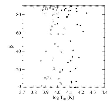
Figure 22: $\beta$-value versus mass (upper panel) and $\beta$-value versus effective temperature (lower panel).

In the upper panel of Fig. 16 we present the distribution of $r$ values for stars of ${\rm M}>3$ ${\rm M}_{\odot}$ and of ${\rm M}<3$ ${\rm M}_{\odot}$ shown by a dotted and a solid line, respectively. The distributions look rather different with an approximately bimodal distribution for lower mass stars with $r$ peaked between $-$0.75 and $-$1 (highest peak) and between 0.25 and 0.5. The highest peak in the distribution of $r$ values for stars with ${\rm M}>3$ ${\rm M}_{\odot}$ is shifted to higher values between $-$0.75 and $-$0.5. Both distributions nearly resemble the $r$ value distribution presented in older studies of Preston ([1967, 1971]) and Landstreet ([1970]), with an apparent deficit of stars with intermediate values of $\beta$. According to probability distributions of $r$ calculated by Landstreet ([1970]), we conclude that the majority of stars in our sample must have a $\beta$ larger 60^∘. The lack of stars with $r$-values near zero can be explained either by an observational effect or by a lack of small $\beta$-values. Further, we note that no star with ${\rm M}>3$ ${\rm M}_{\odot}$ has $r$ larger than 0.5, indicating the difficulty of detecting periodicity in stars with very small magnetic field variations. The examination of the middle panel of Fig. 16 with $r$ values plotted against stellar mass reveals no obvious dependence for lower mass stars whereas higher mass stars with ${\rm M}>{4}$ ${\rm M}_{\odot}$ show a slight trend to have $r<-0.5$. This behaviour can be interpreted by the prevalence of larger obliquities $\beta$ in more massive stars. From the inspection of the dependence between the $r$-values and effective temperatures (lower panel in Fig. 16) the same is possibly true for the hottest stars in our sample, i.e. larger obliquities $\beta$ are found in hotter stars.

Quite interesting results follow from the study of the distribution of $r$-values for stars with different rotation periods and the distribution of $r$-values over the age, i.e. elapsed time on the main sequence presented in Figs. 17 and 18. While we observe a random distribution of obliquity angles $\beta$ in faster rotating stars, it seems that long period magnetic variables of stars with ${\rm M}<3$ ${\rm M}_{\odot}$ tend to have values of $\beta$ close to 0^∘. In the distribution of $r$-values over the age we observe that the obliquity angle distribution as inferred from the distribution of $r$-values appears random at the time magnetic stars become observable on the H-R diagram. After quite a short time spent by a star with mass ${\rm M}<3$ ${\rm M}_{\odot}$ on the main sequence the obliquity angle $\beta$ tends to reach values close to either to 90^∘ or 0^∘. In other words, the magnetic axis becomes either perpendicular to the rotation axis or aligned with it with advanced age. A similar result revealing the bimodal distribution based on a smaller sample of Ap and Bp stars had been presented by North ([1985]), but on the basis of less reliable photometric $\log g$ estimates. For more massive stars with ${\rm M}>3$ ${\rm M}_{\odot}$ the obliquity angle $\beta$ tends to reach values close to 90^∘.

The distribution of obliquity angles $\beta$ for stars with ${\rm M}>3$ ${\rm M}_{\odot}$ and ${\rm M}<3$ ${\rm M}_{\odot}$ is presented in Fig. 19. In agreement with the discussion on the distribution of $r$-values, the excess of stars with large $\beta$-values is detected in both higher and lower mass stars. Recently, Bychkov, Bychkova & Madej ([2004]) presented a study of parameters of magnetic phase curves based on their own compilation in Bychkov, Bychkova & Madej ([2005]) of the data for 134 Ap and Bp stars. Surprisingly, they found an excess of stars with angles $\beta$ close to 0^∘. We do not know the origin of this discrepancy between their and our study, but we only emphasise here that our sample consists of carefully selected 90 Ap and Bp stars with a sufficient number of magnetic field measurements and well-defined periods and magnetic phase curves. From the inspection of plots displaying the distribution of $\beta$ in fast and slowly rotating stars (Fig. 20), it is obvious that large $\beta$ ($\geq$80^∘) outweigh the distributions of faster rotating stars whereas the angle $\beta$ is smaller than 20^∘ in slower rotating stars. We note that all nine points with small values of $\beta$ in slowly rotating stars are from the study of Landstreet & Mathys ([2000]). As for stars with ${\rm M}>3$ ${\rm M}_{\odot}$, the two stars with the longest periods (HD 5737 and HD 168733) have magnetic and rotation axes aligned to within 20^∘, similar to the behaviour of slowly rotating stars of lower mass. Clearly, more magnetic field studies of slowly rotating stars with higher mass are needed to confirm this behaviour.

The evolution of the obliquity angle $\beta$ seems to be quite different for low and high mass stars (Fig. 21). We find a strong hint for an increase of $\beta$ with elapsed time on the main sequence for stars with ${\rm M}>3$ ${\rm M}_{\odot}$. However, no similar trend is found for lower mass stars, although the predominance of high values of $\beta$ at advanced ages is notable. Further, we do not find any trend for $\beta$-values either with mass or with $T_{\rm eff}$ (Fig. 22).

As is mentioned by Bychkov, Bychkova & Madej ([2005]), a number of stars in their catalog exhibit marked anharmonicity, which indicates significant departures from dipole geometry. To reproduce the shapes of the observed longitudinal magnetic field variation, the magnetic field distribution has to be regarded as a sum of dipole and quadrupole components. Out of the 33 stars studied with ${\rm M}>3$ ${\rm M}_{\odot}$, 21% have magnetic phase curves fitted by a double wave, whereas the percentage of stars with ${\rm M}<3$ ${\rm M}_{\odot}$ for which the magnetic field variations had to be fitted by a double wave is 12%. This statistics could indicate the possibility that the magnetic topology in stars with ${\rm M}>3$ ${\rm M}_{\odot}$ is frequently more complex than that in less massive stars. The double-wave longitudinal field curves in stars with ${\rm M}<3$ ${\rm M}_{\odot}$ are mostly found at the age of 40-50% of their main sequence life, while a number of stars with ${\rm M}>3$ ${\rm M}_{\odot}$ exhibit a non-dipolar field already at a very young age close to the ZAMS. However, further systematic studies of mean longitudinal magnetic fields should be conducted to better assert the evolution of the magnetic field distributions during the main-sequence life. Moreover, the observations of other magnetic field moments such as the mean quadratic field and mean crossover field, along with studies of Zeeman structure in the individual line profiles in circular and linear polarisation should be involved in future modeling to obtain a most accurate determination of the magnetic field topologies.

4 Discussion

We believe that the work presented here has important implications for the understanding of the origin of the magnetism detected in A and B stars. The new results based on the statistical properties of 90 Ap and Bp stars can be summarised as follows:

• The present study of the evolutionary state of upper main sequence magnetic stars indicates a notable difference between the distributions of high mass and low mass magnetic stars in the H-R diagram. In contrast to magnetic stars of mass ${\rm M}<3$ ${\rm M}_{\odot}$ which are mostly found around the centre of the main-sequence band, the stars with masses ${\rm M}>3$ ${\rm M}_{\odot}$ seem to be concentrated closer to the ZAMS, and the stronger magnetic fields tend to be found in hotter, younger (in terms of the elapsed fraction of main-sequence life) and more massive stars.

• The longest rotation periods are found in stars in the mass domain between 1.8 and 3 ${\rm M}_{\odot}$ and with $\log g$ values ranging from 3.80 to 4.13. The longest periods are found only in stars which spent already more than 40% of their main sequence life.

• No evidence is found for any loss of angular momentum during the main-sequence life of stars with ${\rm M}>3$ ${\rm M}_{\odot}$.

• No sign of evolution of the magnetic flux over the stellar life time on the main sequence has been found, in agreement with the assumption of magnetic flux conservation.

• Our study of a few known members of nearby open clusters of different ages and with accurate Hipparcos parallaxes confirms the conclusions based on the study of field stars with accurate Hipparcos parallaxes.

• The excess of stars with large obliquities $\beta$ is detected in both higher and lower mass stars. It is quite possible that the angle $\beta$ becomes close to 0^∘ in slower rotating stars of high mass too, analog to the behaviour of angles $\beta$ in slowly rotating stars of ${\rm M}<3$ ${\rm M}_{\odot}$,

• The obliquity angle distribution as inferred from the distribution of $r$-values appears random at the time magnetic stars become observable on the H-R diagram. After quite a short time spent by a star on the main sequence the obliquity angle $\beta$ tends to reach values close to either 90^∘ or 0^∘ for ${\rm M}<3$ ${\rm M}_{\odot}$. However, for ${\rm M}>3$ ${\rm M}_{\odot}$ the obliquity angle $\beta$ in increasing with the completed fraction of the main-sequence life. It would be important to consider such a behaviour in the framework of dynamo or fossil magnetic theories, taking into account the influence of various mechanisms (e.g. possible changes in internal rotation during the evolutionary stage).

• While we find a strong hint for an increase of $\beta$ with the elapsed time on the main sequence for stars with ${\rm M}>3$ ${\rm M}_{\odot}$, the trend for lower mass stars is much less pronounced, though it seems to exist as well.

The presented results have to be implemented in the long-lasting discussions about fossil or dynamo origin for the observed magnetic fields. It is quite possible that the observed magnetic fields in stars with ${\rm M}>3$ ${\rm M}_{\odot}$, showing the prevalence of stronger magnetic fields in younger stars, are in some sense fossil, being the remnants of magnetic fields originally present in the material from which these stars formed. Recent theoretical work indicates that dynamo action is possible, even likely, in a convective core, but the overlying stellar radiative envelope represents a significant impediment to the appearance of any of the generated magnetic field at the surface (e.g., MacGregor & Cassinelli [2003], MacDonald & Mullan [2004]). To remedy the difficulties associated with the transport of magnetic fields from the core to the surface there have been a number of attempts to identify mechanisms that are capable of generating a magnetic field within the radiative envelope itself (e.g., Spruit [2002], Braithwaite [2004], Arlt, Hollerbach & Rüdiger [2003]). For stars with mass ${\rm M}<3$ ${\rm M}_{\odot}$ the magnetic fields appear after they completed more than 20-30% of their main-sequence life. Because of this apparent difference in the evolutionary state between higher mass and older lower mass stars it is tempting to make a conclusion that magnetic fields in stars of lower mass are generated by dynamo action. However, the comparison of the observed magnetic field evolution and magnetic field geometries in both samples presented in this paper does not reveal any striking differences apart from the older age of lower mass magnetic stars on the main sequence, the very fact that most extreme slow rotators are found among stars with ${\rm M}<3$ ${\rm M}_{\odot}$, and the difference in the evolutionary behaviour of obliquities between both samples.