Modeling the Solar Chromosphere

Abstract

Spectral diagnostic features formed in the solar chromosphere are few and difficult to interpret — they are neither formed in the optically thin regime nor in local thermodynamic equilibrium (LTE). To probe the state of the chromosphere, both from observations and theory, it is therefore necessary with modeling. I discuss both traditional semi-empirical modeling, numerical experiments illustrating important ingredients necessary for a self-consistent theoretical modeling of the solar chromosphere and the first results of such models.

Institute of Theoretical Astrophysics, University of Oslo, Norway

1 Introduction

My keynote talk was similar in content to a recent talk at a Sacramento Peak workshop celebrating the 70th birthday of Robert F. Stein. This written version builds to a large extent on that writeup (Carlsson 2006), but it is updated and some sections have been expanded.

Before discussing models of the solar chromosphere it is worthwhile discussing the very definition of the term “chromosphere”. The name comes from the Greek words “$\chi\rho\omega\mu\alpha$” (color) and “$\sigma\varphi\alpha\iota\rho\alpha$” (ball) alluding to the colored thin rim seen above the lunar limb at a solar eclipse. The color comes mainly from emission in the Balmer H$\alpha$ line. This is thus one possible definition — the chromosphere is where this radiation originates. At an eclipse this region has a sharp lower edge, the visible limb, but a fuzzy upper end with prominences protruding into the corona. The nature of this region is difficult to deduce from eclipse observations since we see this region edge on during a very short time span and we have no way of telling whether it is homogeneous along the line of sight or very inhomogeneous in space and time. It was early clear that the emission in H$\alpha$ must mean an atmosphere out of radiative equilibrium — without extra heating the temperature will not be high enough to have enough hydrogen atoms excited to the lower or upper levels of the transition. Early models were constructed to explain observations in H$\alpha$ and in resonance lines from other abundant elements with opacity high enough to place the formation in these regions even in center-of-disk observations (lines like the H and K resonance lines from singly ionized calcium). These early models were constructed assuming one dimensional plane-parallel geometry and they resulted in a temperature falling to a minimum around 4000 K about 500 km above the visible surface, a temperature rise to 8000 K at a height of about 2000 km and then a very rapid temperature rise to a million degree corona. These plane-parallel models have led to a common notion that there is a more or less homogeneous, plane-parallel region between these heights that is hotter than the temperature minimum. In such a picture the chromosphere may be defined as a region occupying a given height range (e.g. between 500 and 2000 km height over the visible surface) or a given temperature range. We may also use physical processes for our definition: the chromosphere is the region above the photosphere where radiative equilibrium breaks down and hydrogen is predominantly neutral (the latter condition giving the transition to the corona). This discussion shows that there is no unique definition of the term “chromosphere”, not even in a one-dimensional, static world. It is even more difficult to agree on a definition of the “chromosphere” that also encompasses an inhomogeneous, dynamic atmosphere.

As mentioned above, the first models of the chromosphere were constructed with a large number of free parameters to match a set of observational constraints. Since some equations are used to restrict the number of free parameters (not all hydrodynamical variables at all points in space and time are determined empirically) we call this class of models semi-empirical models. Typically one assumes hydrostatic equilibrium and charge conservation but no energy equation. The temperature as function of height is treated as a free function to be determined from observations. In the other main class of models one tries to minimize the number of free parameters by including an energy equation. Such theoretical models have been very successful in explaining radiation from stellar photospheres with only the effective temperature, acceleration of gravity and abundances as free parameters. In the chromosphere, an additional term is needed in the energy equation — e.g. energy deposition by acoustic shocks or energy input in connection with magnetic fields (e.g. currents or reconnection).

It is thus clear from observations that the chromosphere is not in radiative equilibrium — there is a net radiative loss. This loss has to be balanced by an energy deposition, at least averaged over a long enough time span, if the atmosphere is to be in equilibrium. This is often called the problem of chromospheric “heating”. It is important to bear in mind, though, that the radiative losses may be balanced by a non-radiative energy input without an increase in the average temperature. The term “chromospheric heating” may thus be misleading since it may be interpreted as implying that the average temperature is higher than what is the case in a radiative equilibrium atmosphere. In the following we will use the term “heating” in a more general sense: a source term in the energy equation, not necessarily leading to an increased temperature.

Chromospheric heating is needed not only for the quiet or average Sun but also in active regions, sunspots and in the outer atmospheres of many other stars. I will in the following mainly discuss the quiet Sun case.

The outline of this paper is as follows: In Section 2 we discuss semi-empirical models of the chromosphere. In Section 3 we discuss theoretical models; first we elaborate on 1D hydrodynamical models, then we discuss the role of high frequency acoustic waves for the heating of the chromosphere and finally we describe recent attempts to model the chromosphere in 3D including the effects of magnetic fields.

2 Semi-empirical Models

Semi-empirical models can be characterized by the set of observations used to constrain the model, the set of physical approximations employed and the set of free parameters to be determined. Spectral diagnostics used to constrain chromospheric models must have high enough opacity to place the formation above the photosphere. The continuum in the optical part of the spectrum is formed in the photosphere so the only hope for chromospheric diagnostics lies in strong spectral lines in this region of the spectrum. Candidates are resonance lines of dominant ionization states of abundant elements and lines from excited levels of the most abundant elements (hydrogen and helium). Most resonance lines are in the UV but the resonance lines of singly ionized calcium (Ca II), called the H and K lines, fulfill our criteria. These lines originate from the ground state of Ca II, the dominant ionization stage under solar chromospheric conditions, and the opacity is therefore given by the density directly and the optical depth is directly proportional to the column mass (i.e. to the total pressure in hydrostatic equilibrium). Also the source function has some coupling to local conditions even at quite low densities (in contrast to the strongly scattering resonance lines of neutral sodium). Other chromospheric diagnostic lines in the optical region are the hydrogen Balmer lines and the helium 1083 nm line. They all originate from highly excited levels and thus have very temperature sensitive opacity. The population of He 1083 is also set by recombination such that its diagnostic potential is very difficult to exploit. With the advent of space based observatories, the full UV spectral range was opened up. Continua shortward of the opacity edge from the ground state of neutral silicon at 152 nm are formed above the photosphere and can be used to constrain chromospheric models. Together with observations in Ly-$\alpha$, such UV continuum observations were used by Vernazza et al. (1973, 1976, 1981) in their seminal series of papers on the solar chromosphere. The VAL3 paper (Vernazza et al. 1981) is one of the most cited papers in solar physics (1072 citations in ADS at the time of writing) and the abstract gives a very concise description of the models and the principles behind their construction: “The described investigation is concerned with the solution of the non-LTE optically thick transfer equations for hydrogen, carbon, and other constituents to determine semi-empirical models for six components of the quiet solar chromosphere. For a given temperature-height distribution, the solution is obtained of the equations of statistical equilibrium, radiative transfer for lines and continua, and hydrostatic equilibrium to find the ionization and excitation conditions for each atomic constituent. The emergent spectrum is calculated, and a trial and error approach is used to adjust the temperature distribution so that the emergent spectrum is in best agreement with the observed one. The relationship between semi-empirical models determined in this way and theoretical models based on radiative equilibrium is discussed by Avrett (1977). Harvard Skylab EUV observations are used to determine models for a number of quiet-sun regions.”

The VAL3 models are thus characterized by them using Ly-$\alpha$ and UV-continuum observations for observational constraint, hydrostatic equilibrium and non-LTE statistical equilibrium in 1D as physical description and temperature as function of height as free function. To get a match with observed line-strengths, a depth-dependent microturbulence was also determined and a corresponding turbulent pressure was added. The number of free parameters to be determined by observations is thus large — in principle the number of depth-points per depth-dependent free function (temperature and microturbulence). In practice the fitting was made by trial and error and only rather smooth functions of depth were tried thus decreasing the degrees of freedom in the optimization procedure.

The models have a minimum temperature around 500 km above the visible surface (optical depth unity at 500 nm), a rapid temperature rise outwards to about 6000 K at 1000 km height and thereafter a gradual temperature increase to 7000 K at 2000 km height with a very rapid increase from there to coronal temperatures.

The Ca II lines were not used in constraining the VAL3 models and the agreement between the model representing the average quiet Sun, VAL3C, and observations of these lines was not good. An updated model with a different structure in the temperature minimum region was published in Maltby et al. (1986) (where the main emphasis was on similarly constructed semi-empirical models for sunspot atmospheres).

A peculiar feature with the VAL models was a temperature plateau introduced between 20000 and 30000 K in order to reproduce the total flux in the Lyman lines. This plateau was no longer necessary in the FAL models where the semi-empirical description of the transition region temperature rise was replaced by the balance between energy flowing down from the corona (conduction and ambipolar diffusion) and radiative losses (Fontenla et al. 1990, 1991, 1993).

One goal of semi-empirical models is to obtain clues as to the non-radiative heating process. From the models it is possible to calculate the amount of non-radiative heating that is needed to sustain the model structure. For the VAL3C model this number is 4.2 kW m^-2 with the dominant radiative losses in lines from Ca II and Mg II, with Ly-$\alpha$ taking over in the topmost part.

The models described so far do not take into account the effect of the very many iron lines. This was done in modeling by Anderson & Athay (1989). Instead of using the temperature as a free parameter and observations as the constraints, they adjusted the non-radiative heating function until they obtained the same temperature structure as in the VAL3C model (arguing that they would then have an equally good fit to the observational constraints as the VAL3C model). The difference in the physical approximations is that they included line blanketing in non-LTE from millions of spectral lines. The radiation losses are dominated by Fe II, with Ca II, Mg II, and H playing important, but secondary, roles. The total non-radiative input needed to balance the radiative losses is three times higher than in the VAL3C model, 14 kW m^-2.

The VAL3 and FAL models show a good fit to the average (spatial and temporal) UV spectrum but fail to reproduce the strong lines from CO. These lines show very low intensities in the line center when observed close to the solar limb, the radiation temperature is as low as 3700 K (Noyes & Hall 1972; Ayres & Testerman 1981; Ayres et al. 1986; Ayres & Wiedemann 1989; Ayres & Brault 1990). If the formation is in LTE this translates directly to a temperature of 3700 K in layers where the inner wings of the H and K lines indicate a temperature of 4400 K. The obvious solution to the problem is that the CO lines are formed in non-LTE with scattering giving a source function below the Planck-function. Several studies have shown that this is not the solution — the CO lines are formed in LTE (e.g. Ayres & Wiedemann 1989; Uitenbroek 2000). The model M_CO constructed to fit the CO-lines (Avrett 1995) give too low UV intensities. One way out is to increase the number of free parameters by abandoning the 1D, one-component, framework and construct a two component semi-empirical atmosphere. The COOLC and FLUXT atmospheric models of Ayres et al. (1986) was such an attempt where a filling factor of 7.5% of the hot flux tube atmosphere FLUXT and 92.5% of the COOLC atmosphere reproduced both the H and K lines and the CO-lines. The UV continua, however, are overestimated by a factor of 20 (Avrett 1995). A combination of 60% of a slightly cooler model than M_CO and 40% of a hot F model provides a better fit (Avrett 1995). Another way of providing enough free parameters for a better fit is to introduce an extra force in the hydrostatic equilibrium equation providing additional support making possible a more extended atmosphere. With this extra free parameter it is possible to construct a 1D temperature structure with a low temperature in the right place to reproduce the near-limb observations of the CO lines and a sharp temperature increase to give enough intensity in the UV continua (Fontenla 2007).

A word of caution is needed here. Semi-empirical models are often impressive in how well they can reproduce observations. This is, however, not a proper test of the realism of the models since the observations have been used to constrain the free parameters. The large number of free parameters (e.g., temperature as function of height, microturbulence as function of height and angle, non-gravitational forces) may hide fundamental shortcomings of the underlying assumptions (e.g., ionization equilibrium, lateral homogeneity, static solution). It is not obvious that the energy input required to sustain a model that reproduces time-averaged intensities is the same as the mean energy input needed in a model that reproduces the time-dependent intensities in a dynamic atmosphere. Semi-empirical modeling may give clues as to what processes may be important but we also need to study these underlying physical processes with fewer free parameters. This is the focus of theoretical models.

3 Theoretical Models

In contrast to semi-empirical models theoretical models include an energy equation. To model the full 3D system with all physical ingredients we know are important for chromospheric conditions is still computationally prohibitive — various approximations have to be made. In one class of modeling one tries to illustrate basic physical processes without the ambition of being realistic enough to allow detailed comparison with observations. Instead the aim is to fashion a basic physical foundation upon which to build our understanding. The other approach is to start with as much realism as can be afforded. Once the models compare favourably with observations, the system is simplified in order to enable an understanding of the most important processes. I here comment on both types of approaches.

3.1 1D radiation hydrodynamic simulations

Acoustic waves were suggested to be the agent of non-radiative energy input already by Biermann (1948) and Schwarzschild (1948). Such waves are inevitably excited by the turbulent motions in the convection zone and propagate outwards, transporting mechanical energy through the photospheric layers into the chromosphere and corona. Due to the exponential decrease of density with height, the amplitude of the waves increases and they steepen into shocks. The theory that the dissipation of shocks heats the outer atmosphere was further investigated by various authors, see reviews by Schrijver (1995); Narain & Ulmschneider (1996).

In a series of papers, Carlsson & Stein (1992, 1994, 1995, 1997, 2002a) have explored the effect of acoustic waves on chromospheric structure and dynamics. The emphasis of this modeling was on a very detailed description of the radiative processes and on the direct comparison with observations. The full non-LTE rate equations for the most important species in the energy balance (hydrogen, helium and calcium) were included thus including the effects of non-equilibrium ionization, excitation, and radiative energy exchange on fluid motions and the effect of motion on the emitted radiation from these species. To make the calculations computationally tractable, the simulations were performed in 1D and magnetic fields were neglected. To enable a direct comparison with observations, acoustic waves were sent in through the bottom boundary with amplitudes and phases that matched observations of Doppler shifts in a photospheric iron line.

These numerical simulations of the response of the chromosphere to acoustic waves show that the Ca II profiles can be explained by acoustic waves close to the acoustic cut-off period of the atmosphere. The simulations of the behaviour of the Ca II H line reproduce the observed features to remarkable detail. The simulations show that the three minute waves are already present at photospheric heights and the dominant photospheric disturbances of five minute period only play a minor modulating role (Carlsson & Stein 1997). The waves grow to large amplitude already at 0.5 Mm height and have a profound effect on the atmosphere. The simulations show that in such a dynamic situation it is misleading to construct a mean static model (Carlsson & Stein 1994, 1995). It was even questioned whether the Sun has an average temperature rise at chromospheric heights in non-magnetic regions (Carlsson & Stein 1995). The simulations also confirmed the result of Kneer (1980) that ionization/recombination timescales in hydrogen are longer than typical hydrodynamical timescales under solar chromospheric conditions. The hydrogen ionization balance is therefore out of equilibrium and depends on the previous history of the atmosphere. Since the hydrogen ionization energy is an important part of the internal energy equation, this non-equilibrium ionization balance also has a very important effect on the energetics and temperature profile of the shocks (Carlsson & Stein 1992, 2002a). Kneer (1980) formulated this result as strongly as “Unless confirmed by consistent dynamical calculations, chromospheric models based on the assumption of statistical steady state should be taken as rough estimates of chromospheric structure.”

Are observations in other chromospheric diagnostics than the Ca II lines consistent with the above mentioned radiation-hydrodynamic simulations of the propagation of acoustic waves? The answer is “No”. The continuum observations around 130 nm are well matched by the simulations (Judge et al. 2003) but continua formed higher in the chromosphere have higher intensity in the observations than in the simulations (Carlsson & Stein 2002c). The chromospheric lines from neutral elements in the UV range are formed in the mid to upper chromosphere. They are in emission at all times and at all positions in the observations, and they show stronger emission than in the simulations.

The failure of the simulations to reproduce diagnostics formed in the middle to upper chromosphere gives us information on the energy balance of these regions. The main candidates for an explanation are the absence of magnetic fields in the simulations and the fact that the acoustic waves fed into the computational domain at the bottom boundary do not include waves with frequencies above 20 mHz.

The reason for the latter shortcoming is that the bottom boundary is determined by an observed wave-field and high frequency waves are not well determined observationally. I first explore the possibility that high frequency acoustic waves may account for the increased input and address the issue of magnetic fields in the next section.

3.2 High frequency waves

Observationally it is difficult to detect high frequency acoustic waves for two reasons: First, the seeing blurs the ground based observations and makes these waves hard to observe. Second, for both ground based and space based observations the signal we get from high frequency waves is weakened by the width of the response function. Wunnenberg et al. (2002) have summarized the various attempts at detecting high frequency waves, and we refer to them for further background.

Theoretically it is also non-trivial to determine the spectrum of generated acoustic waves from convective motions. Analytic studies indicate that there is a peak in the acoustic spectrum around periods of 50 s (Musielak et al. 1994; Fawzy et al. 2002) while results from high-resolution numerical simulations of convection indicate decreasing power as a function of frequency (Goldreich et al. 1994; Stein & Nordlund 2001).

Recently, Fossum & Carlsson (2005b) & Fossum & Carlsson (2006) analyzed observations from the Transition Region And Coronal Explorer (TRACE) satellite in the 1600 Å passband. Simulations were used to get the width of the response function (Fossum & Carlsson 2005a) and to calibrate the observed intensity fluctuations in terms of acoustic energy flux as function of frequency at the response height (about 430 km). It was found that the acoustic energy flux at 430 km is dominated by waves close to the acoustic cut-off frequency and the high frequency waves do not contribute enough to be a significant contributor to the heating of the chromosphere. Waves are detected up to 28 mHz frequency, and even assuming that all the signal at higher frequencies is signal rather than noise, still gives an integrated energy flux of less than 500 W m^-2, too small by a factor of ten to account for the losses in the VAL3C model. For the field free internetwork regions used in the TRACE observations it is more appropriate to use the VAL3A model that was constructed to fit the lowest intensities observed with Skylab. It has about 2.2 times lower radiative losses than VAL3C (Avrett 1981) so there is still a major discrepancy. One should also remember that Anderson & Athay (1989) found three times higher energy requirement than in the VAL3C model when they included the radiative losses in millions of spectral lines, dominated by lines from Fe II. As pointed out by Fossum & Carlsson (2006), the main uncertainty in the results is the limited spatial resolution of the TRACE instrument (0.5^′′ pixels corresponding to 1^′′ resolution with a possible additional smearing from the little known instrument PDF): “There is possibly undetected wave power because of the limited spatial resolution of the TRACE instrument. The wavelength of a 40 mHz acoustic wave is 180 km and the horizontal extent may be smaller than the TRACE resolution of 700 km. Several arguments can be made as to why this effect is probably not drastic. Firstly, 5 minute waves are typically 10–20^′′ in coherence, 3 minute waves 5–10^′′. In both cases 3–6 times the vertical wavelength. This would correspond to close to the resolution element for a 40 mHz wave. Secondly, even a point source excitation will give a spherical wave that will travel faster in the deeper parts (because of the higher temperature) and therefore the spherical wavefront will be refracted to a more planar wave. With a distance of at least 500 km from the excitation level it is hard to imagine waves of much smaller extent than that at a height of 400 km. There is likely hidden power in the subresolution scales, especially at high frequencies. Given the dominance of the low frequencies in the integrated power, the effect on the total power should be small. It is possible to quantify the missing power by making artificial observations of 3D hydrodynamical simulations with different resolution. This is not trivial since the results will be dependent on how well the simuation describes the excitation of high frequency waves and their subsequent propagation. Preliminary tests in a 3D hydrodynamical simulation extending from the convection zone to the corona (Hansteen 2004) indicate that the effect of the limited spatial resolution of TRACE on the total derived acoustic power is below a factor of two. Although it is thus unlikely that there is enough hidden subresolution acoustic power to provide the heating for the chromosphere, the effect of limited spatial resolution is the major uncertainty in the determination of the shape of the acoustic spectrum at high frequencies.”

Another effect that goes in the opposite direction is that the analysis assumes that all observed power above 5 mHz corresponds to propagating acoustic waves. Especially at lower frequencies we will also have a signal from the temporal evolotion of small scale structures that in this analysis is mistakenly attributed to wave power.

In a restrictive interpretation the result of Fossum & Carlsson (2005b) is that acoustic heating can not sustain a temperature structure like that in static, semi-empirical models of the Sun. Whether a dynamic model of the chromosphere can explain the observations with acoustic heating alone has to be answered by comparing observables from the hydrodynamic simulation with observations. This was done by Wedemeyer-Böhm et al. (2007). They come to the conclusion that their dynamic model (Wedemeyer et al. 2004) is compatible with the TRACE observations (the limited spatial resolution of the TRACE instrument severly affects the synthetic observations) and that acoustic waves could provide enough heating of the chromosphere. The synthetic TRACE images do not take into account non-LTE effects or line opacities. It is also worth noting that the model of Wedemeyer et al. (2004) does not have an average temperature rise in the chromosphere and the dominant wave power is at low frequencies close to the acoustic cut-off and not in the high frequency part of the spectrum. Their study, however, is a major step forward — the question will have to be resolved by more realistic modeling and synthesis of observations paired with high quality observations.

The results by Fossum & Carlsson also show that the neglect of high-frequency waves in the simulations by Carlsson & Stein is not an important omission. Comparing their simulations with observations shows that the agreement is good in the lower chromosphere (Carlsson & Stein 1997; Judge et al. 2003) but lines and continua formed above about 0.8 Mm height have much too low mean intensities. This is probably also true for the Wedemeyer et al. (2004) model (since it has similar mean temperature) but this needs to be checked by proper calculations. It thus seems inevitable that the energy balance in the middle and upper chromosphere is dominated by processes related to the magnetic field. This is consistent with the fact that the concept of a non-magnetic chromosphere is at best valid in the low chromosphere — in the middle to upper chromosphere, the magnetic fields have spread and fill the volume. Even in the photosphere, most of the area may be filled with weak fields or with stronger fields with smaller filling factor (Sanchez Almeida 2005; Trujillo Bueno et al. 2004).

3.3 Comprehensive models in 3D

3D hydrodynamic simulations of solar convection have been very successful in reproducing observations (e.g. Nordlund 1982; Stein & Nordlund 1998; Asplund et al. 2000; Vögler et al. 2005). It would be very natural to extend these simulations to chromospheric layers to study the effect of acoustic waves on the structure, dynamics and energetics of the chromosphere. This approach would then include both the excitation of the waves by the turbulent motions in the convection zone and their subsequent damping and dissipation in chromospheric shocks. For a realistic treatment there are several complications. First, the approximation of LTE that works nicely in the photosphere will overestimate the local coupling in chromospheric layers. The strong lines that dominate the radiative coupling have a source function that is dominated by scattering. Second, shock formation in the chromosphere makes it necessary to have a fine grid or describe sub-grid physics with some shock capturing scheme. Third, it is important to take into account the long timescales for hydrogen ionization/recombination for the proper evaluation of the energy balance in the chromosphere (Kneer 1980; Carlsson & Stein 1992, 2002a).

Skartlien (2000) addressed the first issue by extending the multi-group opacity scheme of Nordlund to include the effects of coherent scattering. This modification made it possible to make the first consistent 3D hydrodynamic simulations extending from the convection zone to the chromosphere (Skartlien et al. 2000). Due to the limited spatial resolution, the emphasis was on the excitation of chromospheric wave transients by collapsing granules and not on the detailed structure and dynamics of the chromosphere.

3D hydrodynamic simulations extending into the chromosphere with higher spatial resolution were performed by Wedemeyer et al. (2004). They employed a much more schematic description of the radiation (gray radiation) and did not include the effect of scattering. This shortcoming will surely affect the amount of radiative damping the waves undergo in the photosphere. The neglect of strong lines avoids the problem of too strong coupling with the local conditions induced by the LTE approximation so in a way two shortcomings partly balance out. The chromosphere in their simulations is very dynamic and filamentary. Hot gas coexists with cool gas at all heights and the gas is in the cool state a large fraction of the time. As was the case in Carlsson & Stein (1995) they find that the average gas temperature shows very little increase with height while the radiation temperature does have a chromospheric rise similar to the VAL3C model. The temperature variations are very large, with temperatures as low as 2000 K and as high as 7000 K at a height of 800 km. It is likely that the approximate treatment of the radiation underestimates the amount of radiative damping thus leading to too large an amplitude.

The low temperatures in the simulations allow for a large amount of CO to be present at chromospheric heights, consistent with observations. For a proper calculation of CO concentrations it is important to take into account the detailed chemistry of CO formation, including the timescales of the reactions. This was done in 1D radiation hydrodynamic models by Asensio Ramos et al. (2003) and in 2D models by Wedemeyer-Böhm et al. (2005). The dynamic formation of CO was also included in the 3D models and it was shown that CO-cooling does not play an important role for the dynamic energy balance at chromospheric heights (Wedemeyer-Böhm & Steffen 2007).

Including long timescales for hydrogen ionization/recombination is non-trivial. In a 1D simulation it is still computationally feasible to treat the full non-LTE problem in an implicit scheme (avoiding the problem of stiff equations) as was shown by Carlsson & Stein. The same approach is not possible at present in 3D; the non-local coupling is too expensive to calculate. Fortunately, the hydrogen ionization is dominated by collisional excitation to the first excited level (local process) followed by photo-ionization in the Balmer continuum. Since the radiation field in the Balmer continuum is set in the photosphere, it is possible to describe the photoionization in the chromospheric problem with a fixed radiation field (thus non-local but as a given rate that does not change with the solution). This was shown to work nicely in a 1D setting by Sollum (1999). Leenaarts & Wedemeyer-Böhm (2006) implemented the rate equations in 3D but without the coupling back to the energy equation. The non-equilibrium ionization of hydrogen has a dramatic effect on the ionization balance of hydrogen in the chromosphere in their simulation.

Magnetic fields start to dominate over the plasma somehere in the chromosphere. Chromospheric plasma as seen in the center H$\alpha$ (e.g., Rutten (2007), De Pontieu et al. (2007)) is very clearly organized along the magnetic structures. It is very likely that acoustic heating alone is not sufficient to account for the radiative losses in the chromosphere. It is thus of paramount importance to include magnetic fields in chromospheric modeling but unfortunetely the inclusion of magnetic fields increase the level of complexity enormously. As was the case with acoustic waves, it is necessary to perform numerical experiments and modeling in simplified cases in order to fashion a basic physical foundation upon which to build our understanding. A number of authors have studied various magnetic wave modes and how they couple, see Bogdan et al. (2003) and Khomenko & Collados (2006) for references. Rosenthal et al. (2002) and Bogdan et al. (2003) reported on 2D simulations in various magnetic field configurations in a gravitationally stratified isothermal atmosphere, assuming an adiabatic equation of state. Carlsson & Stein (2002b) and Carlsson & Bogdan (2006) reported on similar calculations in the same isothermal atmosphere but this time in 3D and also studying the effect of radiative damping of the shocks. Hasan et al. (2005) studied the dynamics of the solar magnetic network in two dimensions and Khomenko & Collados (2006) studied the propagation of waves in and close to a structure similar to a small sunspot.

The picture that emerges from these studies is that waves undergo mode conversion, refraction and reflection at the height where the sound speed equals the Alfvén speed (which is typically some place in the chromosphere). The critical quantity for mode conversion is the angle between the magnetic field and the k-vector: the attack angle. At angles smaller than 30 degrees much of the acoustic, fast mode from the photosphere is transmitted as an acoustic, slow mode propagating along the field lines. At larger angles, most of the energy is refracted/reflected and returns as a fast mode creating an interference pattern between the upward and downward propagating waves. When damping from shock dissipation and radiation is taken into account, the waves in the low-mid chromosphere have mostly the character of upward propagating acoustic waves and it is only close to the reflecting layer we get similar amplitudes for the upward propagating and refracted/reflected waves. It is clear that even simple magnetic field geometries and simple incident waves create very intricate interference patterns. In the chromosphere, where the wave amplitude is expected to be large, it is crucial to include the effects of the magnetic fields to understand the structure, dynamics and energetics of the atmosphere. This is true even in areas comparably free of magnetic field (such regions may exist in the lower chromosphere).

The fact that wave propagation is much affected by the magnetic field topology in the chromosphere can be used for “seismology” of the chromosphere. Observational clues have been obtained by McIntosch and co-workers: McIntosh et al. (2001) & McIntosh & Judge (2001) find a clear correlation between observations of wave power in SOHO/SUMER observations and the magnetic field topology as extrapolated from SOHO/MDI observations. These results were extended to the finding of a direct correlation between reduced oscillatory power in the 2D TRACE UV continuum observations and the height of the magnetic canopy (McIntosh et al. 2003) and the authors suggest using TRACE time-series data as a diagnostic of the plasma topography and conditions in the mid-chromosphere through the signatures of the wave modes present. Such helioseismic mapping of the magnetic canopy in the solar chromosphere was performed by Finsterle et al. (2004) and in a coronal hole by McIntosh et al. (2004).

The chromosphere is very inhomogeneous and dynamic. There is no simple way of inverting the above observations to a consistent picture of the chromospheric conditions. One will have to rely on comparisons with full 3D Radiation-Magneto-Hydrodynamic forward modeling. Steiner et al. (2007) tracked a plane-parallel, monochromatic wave propagating through a non-stationary, realistic atmosphere, from the convection-zone through the photosphere into the magnetically dominated chromosphere. They find that a travel time analysis, like the ones mentioned above, indeed is correlated with the magnetic topography and that high frequency waves can be used to extract information on the magnetic canopy.

Including not only 3D hydrodynamics but in addition the magnetic field, and extending the computational domain to include the corona is a daunting task. However, the development of modern codes and computational power is such that it is a task that is within reach of fulfillment. Hansteen (2004) reported on the first results from such comprehensive modeling. The 3D computational box is $16\times 8\times 12$ Mm in size extending 2 Mm below and 10 Mm above the photosphere. Radiation is treated in detail, using multi-group opacities including the effect of scattering (Skartlien 2000), conduction along field-lines is solved for implicitly and optically thin losses are included in the transition region and corona. For a snapshot of such a simulation, see Fig.1.

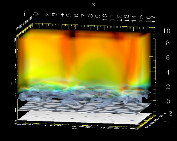
Figure 1.: Temperature structure in a 3D simulation box. The bottom plane shows the temperature at 1.5 Mm below $\tau_{500}$=1 ranging from $15\,700$ K in down-flowing plumes to $16\,500$ in the gas flowing into the simulation domain. The next plane is in the photosphere and shows hot granules and cool intergranular lanes. In the chromosphere the isothermal surfaces show pronounced small scall structures and corrugated shock fronts. The upper 8 Mm is filled with plasma at transition region and coronal temperatures up to 1 MK.

After a relaxation phase from the initial conditions, coronal temperatures are maintained self-consistently by the injection of Pointing flux from the convective buffeting of the magnetic field, much as in the seminal simulations by Gudiksen & Nordlund (2002, 2005a, 2005b).

It is clear from these simulations that the presence of the magnetic field has fundamental importance for chromospheric dynamics and the propagation of waves through the chromosphere. It is also clear that magnetic fields play a role in the heating of the chromosphere (Hansteen et al. 2007).

There are several hotly debated topics in chromospheric modeling today: Is the internetwork chromosphere wholly dynamic in nature or are the dynamic variations only minor perturbations on a semi-static state similar to the state in semi-empirical models (e.g., Kalkofen et al. 1999)? Is there a semi-permanent cold chromosphere (where CO lines originate) or is the CO just formed in the cool phases of a dynamic atmosphere? Is there enough chromospheric heating in high frequency waves of small enough spatial extent that they are not detected by the limited spatial resolution of TRACE? What is the role of the magnetic field (mode conversion of waves, reconection, currents, channeling of waves)? A reason for conflicting results is the incompleteness of the physical description in the modeling and the lack of details (spatial and temporal resolution) in the observations. We are rapidly progressing towards the resolution of this situation. New exciting observations at high temporal and spatial resolution (especially from the Swedish 1-m Solar Telescope on La Palma) are changing our view of the chromosphere. New observing facilities are on the verge of coming on line (GREGOR, Hinode). On the modeling side, several groups have developed codes that start to include the most important ingredients for a comprehensive modeling of the dynamic chromosphere (e.g., Hansteen 2004; Schaffenberger et al. 2006). There is still more work to do with simulations of idealized cases to build up a foundation for our understanding and this is also a field with several groups active at present. The future for chromospheric modeling thus looks both promising and exciting.

Acknowledgments.

This work was supported by the Research Council of Norway grant 146467/420 and a grant of computing time from the Program for Supercomputing.

References

- Anderson & Athay (1989) Anderson L. S., Athay R. G., 1989, ApJ 336, 1089
- Asensio Ramos et al. (2003) Asensio Ramos A., Trujillo Bueno J., Carlsson M., Cernicharo J., 2003, ApJ 588, L61
- Asplund et al. (2000) Asplund M., Nordlund Å., Trampedach R., Allende Prieto C., Stein R. F., 2000, A&A 359, 729
- Avrett (1981) Avrett E., 1981, in R.M.Bonnet, A.K.Dupree (eds.), Solar Phenomena in Stars and Stellar Systems, Dordrecht, 173
- Avrett (1995) Avrett E. H., 1995, in J. R. Kuhn, M. J. Penn (eds.), Infrared tools for solar astrophysics: What’s next?, 303
- Ayres & Brault (1990) Ayres T. R., Brault J. W., 1990, ApJ 363, 705
- Ayres & Testerman (1981) Ayres T. R., Testerman L., 1981, ApJ245, 1124
- Ayres et al. (1986) Ayres T. R., Testerman L., Brault J. W., 1986, ApJ304, 542
- Ayres & Wiedemann (1989) Ayres T. R., Wiedemann G. R., 1989, ApJ338, 1033
- Biermann (1948) Biermann L., 1948, Zs. f. Astrophys. 25, 161
- Bogdan et al. (2003) Bogdan T. J., Carlsson M., Hansteen V., McMurry A., Rosenthal C., Johnson M., Petty-Powell S., Zita E., Stein R., McIntosh S., Nordlund Å., 2003, ApJ 599, 626
- Carlsson (2006) Carlsson M., 2006, in H.Uitenbroek, J.Leibacher, R.F.Stein (eds.), Solar MHD: Theory and Observations - a High Spatial Resolution Perspective, ASP Conf. Ser. 354, 291
- Carlsson & Bogdan (2006) Carlsson M., Bogdan T. J., 2006, Phil. Trans. R. Soc. A 364, 395
- Carlsson & Stein (1992) Carlsson M., Stein R. F., 1992, ApJ 397, L59
- Carlsson & Stein (1994) Carlsson M., Stein R. F., 1994, in M. Carlsson (ed.), Proc. Mini-Workshop on Chromospheric Dynamics, Institute of Theoretical Astrophysics, Oslo, 47
- Carlsson & Stein (1995) Carlsson M., Stein R. F., 1995, ApJ 440, L29
- Carlsson & Stein (1997) Carlsson M., Stein R. F., 1997, ApJ 481, 500
- Carlsson & Stein (2002a) Carlsson M., Stein R. F., 2002a, ApJ 572, 626
- Carlsson & Stein (2002b) Carlsson M., Stein R. F., 2002b, in H. Sawaya-Lacoste (ed.), Magnetic Coupling of the Solar Atmosphere, ESA SP-505, 293
- Carlsson & Stein (2002c) Carlsson M., Stein R. F., 2002c, in A.Wilson (ed.), SOHO-11: From Solar Minimum to Maximum, ESA SP-508, 245
- Fawzy et al. (2002) Fawzy D., Rammacher W., Ulmschneider P., Musielak Z. E., Stȩpień K., 2002, A&A 386, 971
- Finsterle et al. (2004) Finsterle W., Jefferies S. M., Cacciani A., Rapex P., McIntosh S. W., 2004, ApJ 613, L185
- Fontenla (2007) Fontenla J., 2007, in P. Heinzel, I. Dorotovič, R.J. Rutten (eds.), The Physics of the Chromospheric Plasmas, ASP Conf. Ser. 368, 499
- Fontenla et al. (1990) Fontenla J. M., Avrett E. H., Loeser R., 1990, ApJ 355, 700
- Fontenla et al. (1991) Fontenla J. M., Avrett E. H., Loeser R., 1991, ApJ 377, 712
- Fontenla et al. (1993) Fontenla J. M., Avrett E. H., Loeser R., 1993, ApJ 406, 319
- Fossum & Carlsson (2005a) Fossum A., Carlsson M., 2005a, ApJ 625, 556
- Fossum & Carlsson (2005b) Fossum A., Carlsson M., 2005b, Nature 435, 919
- Fossum & Carlsson (2006) Fossum A., Carlsson M., 2006, ApJ 646, 579
- Goldreich et al. (1994) Goldreich P., Murray N., Kumar P., 1994, ApJ 424, 466
- Gudiksen & Nordlund (2002) Gudiksen B. V., Nordlund Å., 2002, ApJ 572, L113
- Gudiksen & Nordlund (2005a) Gudiksen B. V., Nordlund Å., 2005a, ApJ 618, 1031
- Gudiksen & Nordlund (2005b) Gudiksen B. V., Nordlund Å., 2005b, ApJ 618, 1020
- Hansteen et al. (2007) Hansteen V., Carlsson M., Gudiksen B., 2007, in P. Heinzel, I. Dorotovič, R.J. Rutten (eds.), The Physics of the Chromospheric Plasmas, ASP Conf. Ser. 368, 107
- Hansteen (2004) Hansteen V. H., 2004, in A.V.Stepanov, E.E.Benevolenskaya, E.G.Kosovichev (eds.), IAU Symp. 223: Multi Wavelength Investigations of Solar Activity, 385
- Hasan et al. (2005) Hasan S. S., van Ballegooijen A. A., Kalkofen W., Steiner O., 2005, ApJ 631, 1270
- Judge et al. (2003) Judge P. G., Carlsson M., Stein R. F., 2003, ApJ 597, 1158
- Kalkofen et al. (1999) Kalkofen W., Ulmschneider P., Avrett E. H., 1999, ApJ 521, L141
- Khomenko & Collados (2006) Khomenko E., Collados M., 2006, ApJ653, 739
- Kneer (1980) Kneer F., 1980, A&A87, 229
- Leenaarts & Wedemeyer-Böhm (2006) Leenaarts J., Wedemeyer-Böhm S., 2006, A&A460, 301
- Maltby et al. (1986) Maltby P., Avrett E. H., Carlsson M., Kjeldseth-Moe O., Kurucz R. L., Loeser R., 1986, ApJ 306, 284
- McIntosh et al. (2001) McIntosh S. W., Bogdan T. J., Cally P. S., Carlsson M., Hansteen V. H., Judge P. G., Lites B. W., Peter H., Rosenthal C. S., Tarbell T. D., 2001, ApJ 548, L237
- McIntosh et al. (2003) McIntosh S. W., Fleck B., Judge P. G., 2003, A&A 405, 769
- McIntosh et al. (2004) McIntosh S. W., Fleck B., Tarbell T. D., 2004, ApJ 609, L95
- McIntosh & Judge (2001) McIntosh S. W., Judge P. G., 2001, ApJ 561, 420
- Musielak et al. (1994) Musielak Z. E., Rosner R., Stein R. F., Ulmschneider P., 1994, ApJ 423, 474
- Narain & Ulmschneider (1996) Narain U., Ulmschneider P., 1996, Space Sc. Rev. 75, 453
- Nordlund (1982) Nordlund Å., 1982, A&A 107, 1
- Noyes & Hall (1972) Noyes R. W., Hall D. N. B., 1972, ApJ 176, L89
- De Pontieu et al. (2007) De Pontieu B., Hansteen V., van der Voort L. R., van Noort M., Carlsson M., 2007, in P. Heinzel, I. Dorotovič, R.J. Rutten (eds.), The Physics of the Chromospheric Plasmas, ASP Conf. Ser. 368, 65
- Rosenthal et al. (2002) Rosenthal C., Bogdan T., Carlsson M., Dorch S., Hansteen V., McIntosh S., McMurry A., Nordlund Å., Stein R. F., 2002, ApJ 564, 508
- Rutten (2007) Rutten R., 2007, in P. Heinzel, I. Dorotovič, R.J. Rutten (eds.), The Physics of the Chromospheric Plasmas, ASP Conf. Ser. 368, 27
- Sanchez Almeida (2005) Sanchez Almeida J., 2005, A&A 438, 727
- Schaffenberger et al. (2006) Schaffenberger W., Wedemeyer-Böhm S., Steiner O., Freytag B., 2006, in H.Uitenbroek, J.Leibacher, R.F.Stein (eds.), Theory and Observations - a High Spatial Resolution Perspective, ASP Conf. Ser. 354, 351
- Schrijver (1995) Schrijver C., 1995, A&A Rev.6, 181
- Schwarzschild (1948) Schwarzschild M., 1948, ApJ 107, 1
- Skartlien (2000) Skartlien R., 2000, ApJ 536, 465
- Skartlien et al. (2000) Skartlien R., Stein R. F., Nordlund Å., 2000, ApJ 541, 468
- Sollum (1999) Sollum E., 1999, Hydrogen Ionization in the Solar Atmosphere: Exact and Simplified Treatments, MSc Thesis, Institute of Theoretical Astrophysics, University of Oslo, Norway
- Stein & Nordlund (1998) Stein R. F., Nordlund A., 1998, ApJ 499, 914
- Stein & Nordlund (2001) Stein R. F., Nordlund Å., 2001, ApJ 546, 585
- Steiner et al. (2007) Steiner O., Vigeesh G., Krieger L., Wedemeyer-Böhm S., Schaffenberger W., Freytag B., 2007, ArXiv Astrophysics e-prints
- Trujillo Bueno et al. (2004) Trujillo Bueno J., Shchukina N., Asensio Ramos A., 2004, Nature 430, 326
- Uitenbroek (2000) Uitenbroek H., 2000, ApJ536, 481
- Vernazza et al. (1973) Vernazza J. E., Avrett E. H., Loeser R., 1973, ApJ 184, 605
- Vernazza et al. (1976) Vernazza J. E., Avrett E. H., Loeser R., 1976, ApJS 30, 1
- Vernazza et al. (1981) Vernazza J. E., Avrett E. H., Loeser R., 1981, ApJS 45, 635
- Vögler et al. (2005) Vögler A., Shelyag S., Schüssler M., Cattaneo F., Emonet T., Linde T., 2005, A&A429, 335
- Wedemeyer et al. (2004) Wedemeyer S., Freytag B., Steffen M., Ludwig H.-G., Holweger H., 2004, A&A 414, 1121
- Wedemeyer-Böhm et al. (2005) Wedemeyer-Böhm S., Kamp I., Bruls J., Freytag B., 2005, A&A 438, 1043
- Wedemeyer-Böhm & Steffen (2007) Wedemeyer-Böhm S., Steffen M., 2007, A&A, in press
- Wedemeyer-Böhm et al. (2007) Wedemeyer-Böhm S., Steiner O., Bruls J., Ramacher W., 2007, in P. Heinzel, I. Dorotovič, R.J. Rutten (eds.), The Physics of the Chromospheric Plasmas, ASP Conf. Ser. 368, 93
- Wunnenberg et al. (2002) Wunnenberg M., Kneer F., Hirzberger J., 2002, A&A 395, L51