The Phase-resolved High Energy Spectrum of the Crab Pulsar

Abstract

We present a modified outer gap model to study the phase-resolved spectra of the Crab pulsar. A theoretical double peak profile of the light curve containing the whole phase is shown to be consistent with the observed light curve of the Crab pulsar by shifting the inner boundary of the outer gap inwardly to $\sim 10$ stellar radii above the neutron star surface. In this model, the radial distances of the photons corresponding to different phases can be determined in the numerical calculation. Also the local electrodynamics, such as the accelerating electric field, the curvature radius of the magnetic field line and the soft photon energy, are sensitive to the radial distances to the neutron star. Using a synchrotron self-Compton mechanism, the phase-resolved spectra with the energy range from 100 eV to 3 GeV of the Crab pulsar can also be explained.

, , , ,

1 Introduction

There are eight pulsars have been detected in gamma-ray energy range (cf. Thompson 2006 for a recent review) with period ranging from 0.033s to 0.237s and age younger than million years old. Theoretically, it is suggested that high-energy photons are produced by the radiation of charged particles that are accelerated in the pulsar magnetosphere. There are two kinds of theoretical models: one is the polar gap model (e.g., Harding 1981, Daugherty & Harding 1996, for more detail review of polar cap model cf. Harding 2006), and another is the outer gap model (e.g. Cheng, Ho, & Ruderman 1986a, 1986b; Chiang & Romani 1994). Both models predict that electrons and positrons are accelerated in a charge depletion region called a gap by the electric field along the magnetic field lines and assume that charged particles lose their energies via curvature radiation in both polar and outer gaps. The key differences are polar gap are located near stellar surface and the outer gap are located near the null charge surface, where are at least several tens stellar radii away the star.

The continuous observations of powerful young pulsars, including the Crab, the Vela and the Geminga, have collected large number of high energy photons, which allow us to carry out much more detailed analysis. Fierro et al. (1998) divided the whole phase into eight phase intervals, i.e. leading wing 1, peak 1, trailing 1, bridge, leading wing 2, peak 2, trailing 2 and off-pulse. They showed that the data in each of these phases can be roughly fitted with a simple power law. However, the photon indices of these phases are very different, they range from 1.6 to 2.6. Massaro et al. (2000) have shown that X-ray pulse profile is energy dependent and the X-ray spectral index also depends on the phase of the rotation.

The Crab pulsar has been extensively studied from the radio to the extremely high energy ranges, and the phase of the double-pulse with separation of $144^{\circ}$ is found to be consistent over all wavelengths. Recently Kuiper et al. (2001) have combined the X-ray and gamma-ray data of the Crab pulsar, they showed that the phase-dependent spectra exhibit a double-peak structure, i.e. one very broad peak in soft gamma-rays and another broad peak in higher energy gamma-rays. The position of these peaks depend on the phase. Although the double-peak structure is a signature of synchrotron self-Compton mechanism, it is impossible to fit the phase dependent spectrum by a simple particle energy spectrum. Actually it is not surprised that the spectrum is phase dependent because photons are emitted from different regions of the magnetosphere. The local properties, e.g. electric field $E(r)$, magnetic field $B(r)$, particles density and energy distribution are very much different for different regions. Therefore these phase dependent data provide very important information for emission region. Consequently, the phase-resolved properties provide very important clues and constraints for the theoretical models. So far, the three-dimensional outer gap model seems to be the most successful model in explaining both the double-peak pulse profile and the phase-resolved spectra of the Crab pulsar (e.g. Chiang & Romani 1992, 1994; Dyks & Rudak 2003; Cheng, Ruderman & Zhang, 2000, hereafter CRZ). However, the leading-edge and trailing-edge of the light curve cannot be given out, since the inner boundary of the outer gap is located at the null charge surface in this model. Recently, the electro-dynamics of the pulsar magnetosphere has been studied carefully by solving the Poisson equation for electrostatic potential and the Boltzmann equations for electrons/positrons (Hirotani & Shibata, 1999a,b,c; Takata et al. 2004, 2006; Hirotani 2005), and the inner boundary of the gap is shown to be located near the stellar surface.

We will organize the paper as follows. We describe the modified outer gap model in §2. In §3, we calculate the phase-resolved spectra and present the fitting result of the spectra in different phase intervals. Finally, we discuss our results and draw conclusions in §4.

2 A modified outer gap model

Originally proposed by Holloway (1973) that vacuum gaps may form in the outer regions of pulsar’s magnetosphere, Cheng, Ho and Ruderman (1986a, 1986b; hereafter CHR) developed the idea of outer magnetosphere gaps and explained the radiation mechanisms of the $\gamma$-rays from the Crab and Vela pulsars. CHR argued that a global current flowing through the null surface of a rapidly spinning neutron star would result in large regions of charge depletion, which form the gaps in the magnetosphere. They assume the outer gap should begin at the null charge surface and extend to the light cylinder. In the gaps, a large electric field parallel to the magnetic field lines is induced ($\vec{E}\cdot\vec{B}\neq 0$), and it can accelerate the electrons or positrons to extremely relativistic speed. Thus, those charges can emit high energy photons through various mechanisms, and further produce copious $e^{+}e^{-}$ pairs to sustain the gaps and the currents.

Based on the CHR model, Chiang and Romani (1992, 1994) generated gamma ray light curves for various magnetosphere geometries by assuming that gap-type regions could be supported along all field lines which define the boundary between the closed region and open field line region rather than just on the bundle of field lines lying in the plane containing the rotation and magnetic dipole axes. In their model, photons are generated and travel tangential to the local magnetic field lines and there are beams in both the outward and inward directions. They suggested that a single pole would produce a double-peak emission profile when the line of sight crosses the enhanced regions of the $\gamma$-ray beam, while the inner region of the beam results in the bridge emission between these two pulses. The peak phase separation can be accommodated by choosing a proper observer viewing angle. Because the location of emission of each point in phase along a given line of sight can be mapped approximately in this model, the outer gap is thus divided into small subzones. As the curvature radius, photon densities and the local electrodynamics in different subzones are not the same, the spectral variation of the high energy radiation in different phase intervals varies. Later, Romani and Yadigaroglu (1995) developed the single gap model by involving the effects of aberration, retarded potential and time of flight across the magnetosphere. The light curve profiles in this modified model is simply determined by only two parameters, which are magnetic inclination angle $\alpha$ and the viewing angle $\zeta$. They argued that the $\gamma$-ray emission can only be observed from pulsars with large viewing angle ($\zeta\geq 45^{\circ}$), and we cannot receive the $\gamma$ photons but radio emissions from the aligned pulsars ($\alpha\leq 35^{\circ}$). Furthermore, they showed the gap would grow larger as the pulsar slows down, and more open field lines can occupy the outer gap, which means the older pulsar are more efficient for producing GeV $\gamma$-ray photons (Yadigaroglu & Romani, 1995).

However, the assumptions of the model proposed by Romani’s group are not self-consistent. Why is there only a single pole and only outgoing current in the magnetosphere? Cheng, Ruderman and Zhang (2000) proposed another version of three dimensional outer gap model for high energy pulsars based on the pioneering work of Romani, and made it more natural in physics. In the CRZ model, two outer gaps and both outward and inward currents are allowed (though it turns out that outgoing currents dominate the emitted radiation intensities), and the azimuthal extension of the outer gap is restricted on a bundle of fields instead of the whole lines. Like the previous work by Yadigaroglu and Romani (1995), the CRZ model also contains the same two parameters, but more self-consistent in gap geometry and radiation morphology by using the pair production conditions. The electric field parallel to the magnetic field lines is

$$E_{\parallel}=\frac{\Omega B(r)f^{2}(r)R^{2}_{L}}{cs(r)},$$ (1)

where $f(r)\propto r^{3/2}$ and $s(r)\propto r^{1/2}$ are the fractional size of the outer gap and the curvature radius at the distance $r$. The characteristic fractional size of the outer gap evaluated at $r\sim r_{L}$, where $r_{L}$ is the light cylinder radius, can be estimated by the condition of pair creation (Zhang & Cheng 1997; CRZ) and is given by

$$f_{0}=5.5P^{26/21}B_{12}^{-4/7}\Delta\Phi^{1/7}\;\;,$$ (2)

where $\Delta\Phi$ is the azimuthal extension of the outer gap. CRZ estimates its value by considering the local pair production condition and give $\Delta\Phi\sim 160^{\circ}$ for the Crab pular. It has been pointed out that if the inclination angle is small, $f_{0}$ can be changed by a factor of several (Zhang et al. 2004). We want to remark that equation (1) is the solution of vacuum solution, for regions near null surface and the inward extension of the gap the electric field is shown to be deviated from the vacuum solution (e.g Muslimov & Harding 2004; Hirotani 2006). Nevertheless for simplicity we shall assume the vacuum solution for the entire gap.

In the numerical calculation, the outer gap should be divided into several layers in space. The shape of each layer at the stellar surface is similar to that of the polar cap, but smaller in size. Thus, for a thin gap, the calculation of only one representative layer is enough; while for a thick one (e.g. Geminga), several different layers should be added in the calculation (Zhang & Cheng, 2001). The coordinate of the footprint of the last closed field lines on the stellar surface is determined as $(x_{0},y_{0},z_{0})$, then the coordinates values $(x^{\prime}_{0},y^{\prime}_{0},z^{\prime}_{0})$ of the inner layers can be defined by $x^{\prime}_{0}=a_{1}x_{0},~{}y^{\prime}_{0}=a_{1}y_{0},$ and $z^{\prime}_{0}=\sqrt{1-{x^{\prime}_{0}}^{2}-{y^{\prime}_{0}}^{2}}$, where $a_{1}$ corresponds to the various layers in the open volume.

Inside the light cylinder, high energy photons will be emitted nearly tangent to the magnetic field lines in the corotating frame because of the relativistic $1/\gamma$ beaming inherent in high energy processes unless $|\bf{E}\times\bf{B}|\sim B^{2}$. Then the propagation direction of each emitted photons by relativistic charged particles can be expressed as ($\zeta$,$\Phi$), where $\zeta$ is the polar angle from the rotation axis and $\Phi$ is the phase of rotation of the star. Effects of the time of flight and aberration are taken into account. A photon with velocity ${\bf{u}}=(u_{x},u_{y},u_{z})$ along a magnetic field line with a relativistic addition of velocity along the azimuthal angle gives an aberrated emission direction ${\bf{u^{\prime}}}=(u^{\prime}_{x},u^{\prime}_{y},u^{\prime}_{z})$. The time of flight gives a change of the phase of the rotation of the star. Combining these two effects, and choosing $\Phi=0$ for radiation in the (x,z) plane from the center of the star, $\zeta$ and $\Phi$ are given by $\cos\zeta=u^{\prime}_{z}$ and $\Phi=-\phi_{u^{\prime}}-{\vec{r}}\cdot{\hat{u^{\prime}}}$, where $\phi_{u^{\prime}}$ is the azimuthal angle of $\hat{u^{\prime}}$ and $\vec{r}$ is the emitting location in units of $R_{L}$. In panel A of Fig. 1, the emission morphology in the ($\zeta$, $\Phi$) plane is shown. For a given observer with a fixed viewing angle $\zeta$, a double-pulsed structure is observed because photons are clustered near two edges of the emission pattern due to the relativistic effects (cf. panel B of Fig. 1).

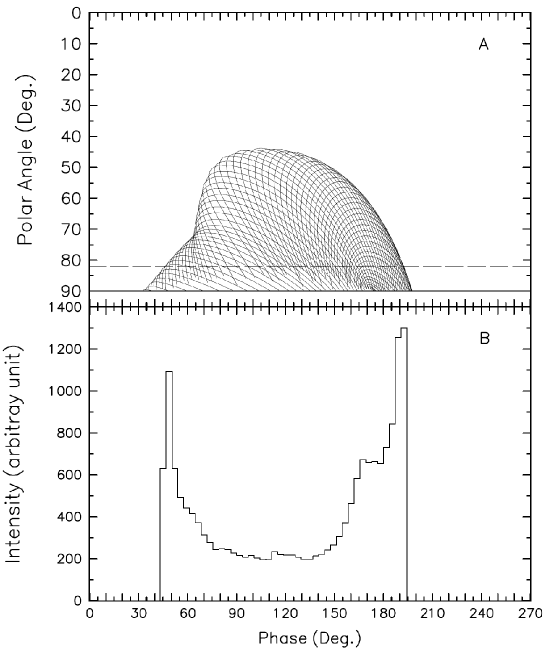
Figure 1: Emission projection onto the ($\zeta$,$\Phi$) plane and pulse profile for the single pole outer gap. The photons are emitted outwards from the outer gap. (a) The emission projection ($a1=0.9$) and (b) the corresponding pulse profile ($\Delta a1=0.03$), for Crab parameters $\alpha=65^{\circ}$ and $\zeta=82^{\circ}$.

In Fig. 1, we can see that this model can only produce radiation between two peaks. However, the observed data of the Crab, Vela and Geminga indicate that the leading wing 1 and the trailing wing 2 are quite strong, and even the intensity in off-pulse cannot be ignored. Hirotani and his co-workers (Hirotani & Shibata 2001; Hirotani, Harding & Shibata 2003) have pointed out that the large current in the outer gap can change the boundary of the outer gap. They solve the set of Maxwell and Boltzmann equations in pulsar magnetospheres and demonstrate the existence of outer-gap accelerators, whose inner boundary position depends the detail of the current flow and it is not necessarily located at the null charge surface. For the gap current lower than 25% of the Goldreich-Julian current, the inner boundary of the outer gap is very close to the null surface (Hirotani 2005). On the other hand if the current is close to the Goldreich-Julian current, the inner boundary can be as close as 10 stellar radii. In Fig. 2, we show the light curve by assuming the inner boundary is extended inward from the null charge surface to 10 stellar radii (cf. panel A of Fig. 2). In panel B of Fig. 2, the solid line represents emission trajectory of outgoing radiation of one gap from the null surface to the light cylinder with $\alpha$ = 50^∘ and $\zeta=75^{\circ}$ and the dashed line represents the outgoing radiation from another gap from the inner boundary to the null surface. In the presence of the extended emission region from the near the stellar surface to the null charge surface, leading wing 1, trailing wing 2 and the off-pulse components can also be produced.

Figure 2: Upper panel: the simulated pulse profile of the Crab pulsar; lower panel: variation of radial distance with pulse phase for the Crab pulsar in units of $R_{L}$, where the bold line represents those in the outer magnetosphere, and the dashed line represents those in the inner magnetosphere. The inclination angle is $50^{\circ}$ and the viewing angle is $75^{\circ}$.

3 The phase-resolved spectra

3.1 radiation spectrum

The Crab pulsar has enough photons for its spectra to be analyzed, and the phase-resolved spectra are useful for study of the local properties of the magnetosphere. Here, we summarize the calculation procedure of the radiation spectrum given in CRZ, which is used to calculate the spectrum in different phases.

The electric field of a thin outer gap (CHR) is given by $E_{\parallel}(r)=\frac{\Omega B(r)a^{2}(r)}{cs(r)}=\frac{\Omega B(r)f^{2}(r)R^{2}_{L}}{cs(r)}$, where $a(r)$ is the thickness of the outer gap at position $r$, and $f(r)=a(r)/R_{L}$ is the local fractional size of the outer gap. Assuming that the magnetic flux subtended in the outer gap is constant in the steady state, we get the local size factor $f(r)\sim f(R_{L})(\frac{r}{R_{L}})^{3/2}$, where $f(R_{L})$ is estimated by using the pair creation condition (cf. Zhang & Cheng 1997, CRZ). As the equilibrium between the energy loss in radiation and gain from accelerating electric field, the local Lorentz factor of the electrons/positrons in the outer gap is $\gamma_{e}(r)=(\frac{3}{2}\frac{s^{2}}{e^{2}c}eE_{\parallel}(r)c)^{1/4}$.

For a volume element $\Delta V$ in the outer gap, the number of primary charged particles can be roughly written as $dN=n_{\rm{GJ}}\Delta A\Delta l$, where $n_{\rm{GJ}}=\frac{\bf{\Omega\cdot B}}{2\pi ec}$ is the local Goldreich-Julian number density, $B\Delta A$ is the magnetic flux through the accelerator and $\Delta l$ is the path length along its magnetic field lines. (Here, We would like to remark that this could overestimate the primary charge number density near the null surface, where the positronic charge density dominates the Goldreich-Julian charge density. However, the observed radiation comes from the wide range of magnetospheric region, an slight overestimation of a small region should not cause a qualitative difference.) Thus, the total number of the charged particles in the outer gap is $N\sim\frac{\Omega\Phi}{4\pi ce}R_{L}$, where $\Phi\sim f(R_{L})B(R_{L})R^{2}_{L}\Delta\phi$ is the typical angular width of the magnetic flux tube subtend in the outer gap. The primary $e^{\pm}$ pairs radiate curvature photons with a characteristic energy $E_{cur}(r)=\frac{3}{2}\hbar\gamma^{3}_{e}(r)\frac{c}{s(r)}$, and the power into curvature radiation for $dN$ $e^{\pm}$ pairs in a unit volume is $\frac{dL_{cur}}{dV}\approx l_{cur}n_{\rm{GJ}}(r)$, where $l_{cur}=eE_{\parallel}c$ is the local power into the curvature radiation from a single electron/positron. The spectrum of primary photons from a unit volume is

$$\frac{d^{2}\dot{N}}{dVdE_{\gamma}}\approx\frac{l_{cur}n_{\rm{GJ}}}{E_{cur}}\frac{1}{E_{\gamma}},~{}~{}E_{\gamma}\leq E_{cur}.$$ (3)

These primary curvature photons collide with the soft photons produced by synchrotron radiation of the secondary $e^{\pm}$ pairs, and produce the secondary $e^{\pm}$ pairs by photon-photon production. In a steady state, the distribution of secondary electrons/positrons in a unit volume is

$$\frac{d^{2}N}{dVdE_{e}}\approx\frac{1}{\dot{E}_{e}}\int\frac{d^{2}\dot{N}(E^{\prime}_{\gamma}=2E^{\prime}_{e})}{dVdE_{\gamma}}dE^{\prime}_{e}\approx\frac{1}{\dot{E}_{e}}\frac{l_{cur}n_{\rm{GJ}}}{E_{cur}}\ln(\frac{E_{cur}}{E_{e}}),$$ (4)

with $\dot{E}_{e}$ the electron energy loss into synchrotron radiation, which is $\dot{E}_{e}=-\frac{2}{3}\frac{e^{4}B^{2}(r)\sin^{2}\beta(r)}{m^{2}_{e}c^{3}}(\frac{E_{e}}{m_{e}c^{2}})^{2}$, where $B(r)$ is the local magnetic field and $\beta(r)$ the local pitch angle, $\sin\beta(r)\sim\sin\beta(R_{L})(\frac{r}{R_{L}})^{1/2}$, $\sin\beta(R_{L})$ is the pitch angle at the light cylinder. Therefore, the energy distribution of the secondary electrons/positrons in volume $\Delta V(r)$ can be written as

$$\frac{dN(r)}{dE_{e}}\approx\frac{d^{2}N}{dVdE_{e}}\Delta V(r)\sim\frac{1}{\dot{E}_{e}}\frac{l_{cur}n_{\rm{GJ}}\Delta V(r)}{E_{cur}}\ln(\frac{E_{cur}}{E_{e}}).$$ (5)

The corresponding photon spectrum of the synchrotron radiation is

$$F_{syn}(E_{\gamma},r)=\frac{\sqrt{3}e^{3}B(r)\sin\beta}{m_{e}c^{2}h}\frac{1}{E_{\gamma}}\int^{E_{max}}_{E_{min}}\frac{dN(r)}{dE_{e}}F(x)dE_{e},$$ (6)

where $x=E_{\gamma}/E_{syn}$, and $E_{syn}(r)=\frac{3}{2}(\frac{E_{e}}{m_{e}c^{2}})^{2}\frac{heB(r)\sin\beta(r)}{m_{e}c}$ is the typical photon energy, and $F(x)=x\int^{\infty}_{x}K_{5/3}(y)dy$, where $K_{5/3}(y)$ is the modified Bessel function of order 5/3. Also, the spectrum of the inverse Compton scattered photons in the volume $\Delta V(r)$ is

$$F_{ICS}(E_{\gamma},r)=\int^{E_{max}}_{E_{min}}\frac{dN(r)}{dE_{e}}\frac{d^{2}N_{ICS}(r)}{dE_{\gamma}dt}dE_{e},$$ (7)

where $\frac{d^{2}N_{ICS}(r)}{dE_{\gamma}dt}=\int^{\epsilon_{2}}_{\epsilon_{1}}n_{syn}(\epsilon,r)F(\%epsilon,E_{\gamma},E_{e})d\epsilon$, and $F(\epsilon,E_{\gamma},E_{e})=\frac{3\sigma_{T}c}{4(E_{e}/mc^{2})^{2}}\frac{1}{\epsilon}[2q\ln q+(1+2q)(1-q)+\frac{(\Gamma q)^{2}(1-q)}{2(1+\Gamma q)}]$, where $\Gamma=4\epsilon(E_{e}/m_{e}c^{2})/m_{e}c^{2}$, $q=E_{1}/\Gamma(1-E_{1})$ with $E_{1}=E_{\gamma}/E_{e}$ and $1/4(E_{e}/m_{e}c^{2})<q<1$. The number density of the synchrotron photons with energy $\epsilon$ is $n_{syn}(\epsilon,r)=\frac{F_{syn}(\epsilon)}{cr^{2}\Delta\Omega}$, where $F_{syn}$ is the calculated synchrotron radiation flux, and $\Delta\Omega$ is the usual beam solid angle.

Figure 3: Phase resolved spectra of the Crab pulsar from 100 eV to 3 GeV in the 7 narrow pulse-phase intervals. Two spectra (for the TW1 and LW2) are displayed twice. The curved line is calculated by the theoretical model, and the observed data are taken from Kuiper et al. (2001).

Fig. 3 shows the observed data of the phase-resolved spectra from 100 eV to 3 GeV of the Crab pulsar, and the theoretical fitting results calculated by using the synchrotron self-Compton mechanism. The phase intervals are defined by division given by Fierro (1998), and the amplitude of the spectrum in each phase interval is proportional to the number of photons counted in it. In this fitting, $f(R_{L})=0.21$, and $B=3.0\times 10^{12}\rm{Gauss}$ are used, which give a consistent fitting of the phase-resolved spectra of the seven phase intervals. In order to obtain a better fit, we treat the pitch angle ($\beta$) and the beam solid angle ($\Delta\Omega$) near the light cylinder as free parameters and vary from phase to phase in the calculation. $\sin\beta(R_{L})=0.06$ and $\Delta\Omega=5.0$ are chosen for trailing wing 1, bridge and leading wing 2; $\sin\beta(R_{L})=0.02,\Delta\Omega=1.0$ for leading wing 1; $\sin\beta(R_{L})=0.04,\Delta\Omega=3.5$ for peak 1, $\sin\beta(R_{L})=0.07,\Delta\Omega=3.0$ for peak 2, and $\sin\beta(R_{L})=0.03,\Delta\Omega=6.0$ for trailing wing 2. Additionally, the phase-averaged spectrum of the total pulse of the Crab pulsar is shown in Fig. 4, where the parameters are chosen as $\sin\beta(R_{L})=0.05$ and $\Delta\Omega=5.0$.

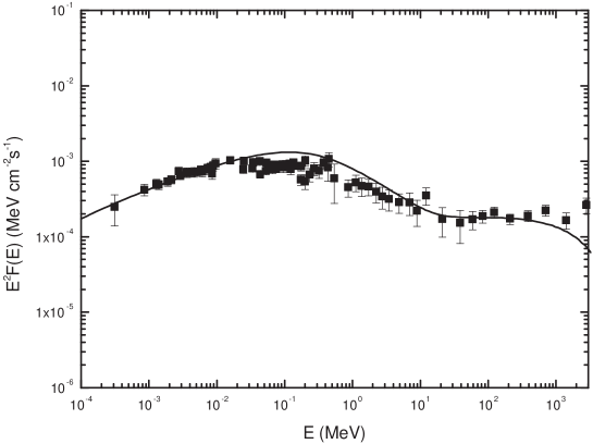
Figure 4: Phase-averaged spectrum of the Crab pulsar. The observed data are taken from Kuiper et al. (2001).

3.2 Analysis of the Phase-Resolved Spectra

The high energy spectra of the Crab pulsar is explained by using the synchrotron self-Compton mechanism, which involves both the synchrotron radiation and the Inverse Compton-Scattering (ICS) caused by the ultra-relativistic electron/positron pairs created by the extremely high-energy curvature photons. The secondary $e^{\pm}$ pairs gyrate in the strong magnetic field and radiate synchrotron photons. While in the far regions of the magnetosphere where the magnetic field decays rapidly, the relativistic pairs collide with the soft synchrotron photons through the ICS process. Thus, the spectra of the radiation contain two main components: one is the synchrotron radiation from the soft X-ray to $\sim$10 MeV, and the other is the ICS component in the even higher energy range. Usually, the synchrotron spectrum has stronger amplitude than that of ICS, and there is obvious turning frequency between these two components, e.g. about 3MeV for peak 1. As we know, the power of synchrotron radiation and ICS can be compared by the ratio of the local magnetic energy density and the photon energy density, i.e.

$$\frac{P_{syn}}{P_{ICS}}\approx\frac{U_{B}}{U_{ph}}\propto\frac{B(r)^{2}/8\pi}{\epsilon_{syn}(r)n_{syn}(\epsilon_{syn},r)},$$ (8)

where $\epsilon_{syn}(r)$ is the synchrotron photon energy in location $r$. In Fig. 3, the spectra in trailing wing 1, bridge and leading wing 2 have broad synchrotron spectra, which cover from 100 eV to $\sim$30 MeV. In Fig. 2, it is demonstrated that the radiation of these three phase intervals are dominated by the photons generated in the near surface region, where the magnetic field is so strong that synchrotron radiation takes up the most emission. However, the radiation of peak 1 and 2 are from the far regions near the light cylinder, where the magnetic field decays rapidly $(B\propto r^{-3})$, thus, the ICS radiation becomes more important above 3 MeV.

The peak of the synchrotron spectrum is determined by the characteristic synchrotron photon energy. Since $E_{syn}\propto\gamma^{2}_{e}B\sin\beta$, where $\gamma_{e}$ is the Lorentz factor of the secondary pairs and $\beta$ is the pitch angle of the electron/positron to the magnetic field, the peak of the synchrotron spectrum can shift if the $\beta$ varies. Since the outward radiation direction covers a wider range than that of the inward radiation, so the solid angle $(\Delta\Omega)$ is no longer the unity as assumed in CRZ model. The solid angle can effect the amplitude of the ICS spectrum because the number density of the synchrotron photons is proportional to $\frac{1}{\Delta\Omega}$. Therefore it is reasonable for us to choose $\beta(R_{L})$ and $\Delta\Omega$ as a set of parameters in fitting the phase-resolved spectra of the Crab pulsar.

4 Conclusion and Discussion

We have tried to explain the high energy light curve and the phase-resolved spectra in the energy range from 100 eV to 3 GeV of the Crab pulsar by modifying the three dimensional outer magnetosphere gap model. Compared to the classical outer gap with the inner boundary at the null charge surface, the modified model allows the outer gap to start at the region about several stellar radii above the neutron star surface, and the ”inwardly-extended” part of the outer gap contributes to the outer wings and off-pulse of the light curve. Such modified outer gap geometry also plays a vital role in explaining the optical polarization properties of the Crab pulsar (Takata et al. 2006). Two adjustable parameters are used to simulate the light curve: one is the inclination angle of the magnetic axis to the rotational axis $\alpha$, and the other is the viewing angle also to the rotational axis $\zeta$. As constrained by the phase separation of the double peaks, we choose the values for these two parameters that $\alpha=50^{\circ}$ and $\zeta=75^{\circ}$. So far, these two parameters have not been determined from the observations. From radio observations, Rankin (1993) estimated that $\alpha\approx 84^{\circ}$ and $\zeta$ is not known. Moffett and Hankins (1999) gave that $\alpha\approx 56^{\circ}$ and $\zeta=117^{\circ}$ by using the polarimetric observations at frequencies between 1.4 and 8.4 GHz. Of course, our values cannot be the true ones, and require further observations to give strong restrictions of them.

In fitting the phase-resolved spectra of the Crab pulsar, our model performs well from 100 eV to 1 GeV, but fails beyond 1 GeV. The inverse Compton scattering spectrum of our results falls down quickly when the energy is over 1 GeV, but the observation data indicates that the spectrum still increases, especially in the first trailing wing, the bridge and the second leading wing phase intervals. We have assumed that the curvature photons are all absorbed by the magnetic field lines, however, some of these multi-GeV photons produced near the light cylinder should be easily escaped from the photon-photon pair creation process. In the spectrum fitting of peak 1, our result has a frequency shift below 1 MeV, and we found that in order to well fit the spectrum we should reduce the curvature photon energy by a quarter. The energy of the curvature photon $E_{cur}\propto s^{-1}(r)$, where $s(r)$ is the local curvature radius. As the high energy photons are produced in the far regions of the magnetosphere, where $s(r)$ maybe not follow the dipole form, we can change the photon energy slightly.

Moreover, the stellar radius of a neutron star is usually treated as $10^{6}$ cm when calculating the strength of the surface magnetic field. However, the equation of state inside the neutron star of the current theoretical models cannot give a convincing value of the neutron star size. Thus, we can only determine the magnetic moment, i.e. $B_{p}R^{3}_{0}$, of the pulsar from the energy loss rate. Therefore, we can rewrite the magnetic field of the Crab pulsar as $B_{12}R^{3}_{6}=3.8$. In fitting the phase-resolved spectra of the Crab pulsar, we choose $B_{p}=3\times 10^{12}$ G, not the traditional value of $3.8\times 10^{12}$ G, for it gives a better fitting on the lower energy range below 10 keV.

Finally we want to emphasize that

This research is supported by a RGC grant of Hong Kong Government under HKU 7015/05P.

References

- Cheng, Ho & Ruderman (1986a) Cheng, K.S., Ho, C., & Ruderman, M.A., Energetic radiation from rapidly spinning pulsars. I - Outer magnetosphere gaps, 1986a, ApJ, 300, 500-521. (CHR)
- Cheng, Ho & Ruderman (1986b) Cheng, K.S., Ho, C., & Ruderman, M.A., Energetic radiation from rapidly spinning pulsars. II. VELA and Crab, 1986b, ApJ, 300, 522-539.
- Cheng, Ruderman & Zhang (2000) Cheng, K.S., Ruderman, M.A., & Zhang, L., A three-dimensional outer magnetospheric gap model for gamma-ray pulsars: geometry, pair production, emission morphologies, and phase-resolved spectra, 2000, ApJ, 537, 964-976. (CRZ)
- Chiang & Romani (1992) Chiang, J., & Romani, R.W., Gamma radiation from pulsar magnetospheric gaps, 1992, ApJ, 400, 629-637.
- Chiang & Romani (1994) Chiang, J., & Romani, R.W., An outer gap model of high-energy emission from rotation-powered pulsars, 1994, ApJ, 436, 754-761.
- Daugherty & Harding (1996) Daugherty, J.K., & Harding, A.K., Gamma-ray pulsars: Emission from extended polar CAP cascades, 1996, ApJ, 458, 278-292.
- Dyks & Rudak (2003) Dyks, J., & Rudak, B., Two-Pole Caustic Model for High-Energy Light Curves of Pulsars, 2003, ApJ, 598, 1201-1206.
- Fierro et al. (1998) Fierro, J.M., Michelson, P.F., Nolan , P.L., & Thompson, D.J., Phase-resolved studies of the high-energy gamma-ray emission from the Crab, Geminga, and VELA pulsars, 1998, ApJ, 494, 734-746.
- Harding (1981) Harding, A.K., Pulsar gamma-rays - Spectra, luminosities, and efficiencies, 1981, ApJ, 245, 267-273.
- Harding (2006) Harding, A.K., Pulsar Acceleration and High Pulsar Acceleration and High- Energy Emission from the Polar Cap and Slot Gap, 2006, in 363rd Heraeus Seminar: Neutron Stars and Pulsars Bad Honnef 14-19 May 2006
- Hirotani (2005) Hirotani, K., Gamma-ray emission from pulsar outer magnetospheres, 2005, Ap&SS, 297, 81-91.
- Hirotani (2005) Hirotani, K., High energy emission from pulsars: Outer gap scenario, 2005, AdSpR, 35, 1085-1091.
- Hirotani (2006)
- Hirotani, Harding & Shibata (2003) Hirotani, K., Harding, A.K., & Shibata, S., Electrodynamics of an outer gap accelerator: Formation of a soft power-law spectrum between 100 MeV and 3 GeV, 2003, ApJ, 591, 334-353.
- Hirotani & Shibata (1999a) Hirotani, K., & Shibata, S., One-dimensional electric field structure of an outer gap accelerator - I. gamma-ray production resulting from curvature radiation, 1999a, MNRAS, 308, 54-66.
- Hirotani & Shibata (1999b) Hirotani, K., & Shibata, S., One-dimensional electric field structure of an outer gap accelerator - II. gamma-ray production resulting from inverse Compton scattering, 1999b, MNRAS, 308, 67-76.
- Hirotani & Shibata (1999c) Hirotani, K., & Shibata, S., Gamma-ray emission from pulsar outer magnetosphere: spectra of curvature radiation, 1999c, PASJ, 51, 683-691.
- Hirotani & Shibata (2001) Hirotani, K., & Shibata, S., Electrodynamic structure of an outer gap accelerator: Location of the gap and the gamma-ray emission from the Crab pulsar, 2001, ApJ, 558, 216-227.
- Hirotani & Shibata (2001) Hirotani, K., & Shibata, S., One-dimensional electric field structure of an outer gap accelerator - III. Location of the gap and the gamma-ray spectrum, 2001, MNRAS, 325, 1228-1240.
- Holloway (1973) Holloway, N.J., Pulsars-p-n junctions in pulsar magnetospheres, 1973, Nature, 246, 6.
- Kuiper et al. (2001) Kuiper, L., Hermsen, W., Cusumano , G., Diehl, R., Schönfelder, V., Strong, A., Bennett, K., & McConnell, M.L., The Crab pulsar in the 0.75-30 MeV range as seen by CGRO COMPTEL. A coherent high-energy picture from soft X-rays up to high-energy gamma-rays, 2001, A&A, 378, 918-935.
- Massaro et al. (2000) Massaro, E., Cusumano, G., Litterio, M., & Mineo, T., Fine phase resolved spectroscopy of the X-ray emission of the Crab pulsar (PSR B0531+21) observed with BeppoSAX, 2000, A&A, 361, 695-703.
- Moffett & Hankins (1999) Moffett, D.A., & Hankins, T.H., Polarimetric properties of the Crab pulsar between 1.4 and 8.4 GHz, 1999, ApJ, 522, 1046-1052.
- Rankin (1993) Rankin, J.M., Toward an empirical theory of pulsar emission. VI - The geometry of the conal emission region, 1993, ApJ, 405, 285-297.
- Romani & Yadigaroglu (1995) Romani, R.W., & Yadigaroglu, I.A., Gamma-ray pulsars: Emission zones and viewing geometries, 1995, ApJ, 438, 314-321.
- Takata, Chang & Cheng (2006) Takata, J., Chang , H.K., & Cheng, K.S., Polarization of high energy emission from the Crab pulsar, 2007, ApJ, 656, 1044-1055.
- Takata, Shibata & Hirotani (2004) Takata, J., Shibata , S., & Hirotani, K., Outer-magnetospheric model for Vela-like pulsars: formation of sub-GeV spectrum, 2004, MNRAS, 348, 241-249.
- Takata, Shibata & Hirotani (2004) Takata, J., Shibata , S., & Hirotani, K., A pulsar outer gap model with trans-field structure, 2004, MNRAS, 354, 1120-1132.
- Takata (2006) Takata, J.; Chang, H. -K.; Cheng, K. S., Polarization of high-energy emissions from the Crab pulsar, 2006, ApJ, in press (astro-ph/0610348).
- Thompson (2006) Thompson, D.J., Future Gamma Future Gamma-Ray Ray Observations of Pulsars and Observations of Pulsars and their Environments their Environments, 2006, in 363rd Heraeus Seminar: Neutron Stars and Pulsars Bad Honnef 14-19 May 2006.
- Yadigaroglu & Romani (1995) Yadigaroglu, I.A., & Romani, R.W., Gamma-ray pulsars: beaming evolution, statistics, and unidentified EGRET sources, 1995, ApJ, 449, 211-215.
- Zhang & Cheng (1997) Zhang, L., & Cheng, K.S., High-energy radiation from rapidly spinning pulsars with thick outer gaps, 1997, ApJ, 487, 370-379.
- Zhang & Cheng (2001) Zhang, L., & Cheng, K.S., Gamma-ray pulsars: the pulse profiles and phase-resolved spectra of Geminga, 2001, MNRAS, 320, 477-484.
- Zhang et al. (2004) Zhang, L., Cheng, K. S., Jiang, Z. J. & Leung, P., Gamma-Ray Luminosity and Death Lines of Pulsars with Outer Gaps, 2004, ApJ, 604, 317-327.