A New Monte Carlo Method and Its Implications for Generalized Cluster Algorithms

Abstract

We describe a novel switching algorithm based on a “reverse” Monte Carlo method, in which the potential is stochastically modified before the system configuration is moved. This new algorithm facilitates a generalized formulation of cluster-type Monte Carlo methods, and the generalization makes it possible to derive cluster algorithms for systems with both discrete and continuous degrees of freedom. The roughening transition in the sine-Gordon model has been studied with this method, and high-accuracy simulations for system sizes up to $1024^{2}$ were carried out to examine the logarithmic divergence of the surface roughness above the transition temperature, revealing clear evidence for universal scaling of the Kosterlitz-Thouless type.

Large-scale Monte Carlo (MC) simulations are often plagued by slow sampling problems. These problems are especially severe in systems near the critical point or in those with strong correlations. Slow sampling problems manifest themselves as poor scaling of the dynamic relaxation time with the system size, making large-size simulations extremely slow to converge. The cause of these problems is that most MC simulations are based on local moves, and when the correlation length of the system grows or as relaxation modes of the system become heavily entangled, local moves become increasingly inefficient. But if nonlocal MC moves are used ref1 , their acceptance ratios are often found to be exceedingly low when system correlations are strong.

One way to circumvent these problems was suggested by Swendsen and Wang 87swe86 , who devised a clever scheme where large-scale nonlocal MC moves may be constructed to achieve high sampling efficiencies by exploiting certain geometric symmetries in the system. This algorithm led to a marked reduction in the dynamical scaling exponent in the 2-dimensional Ising model near criticality. Since the nonlocal moves in this algorithm update a large number of degrees of freedom at the same time, the Swendsen-Wang method and others inspired by it are also often referred to as “cluster Monte Carlo” methods.

Since Swendsen and Wang’s paper in 1987, many cluster-type MC algorithms have appeared 88edw2009 ; 88kan1591 ; 88wol1461 ; 88nie2026 ; 89wol361 ; 90kan941 ; 90wan565 ; 91kan8539 ; 91eve185 ; 92lia2145 ; 92has10472 ; 94has255 ; 95dre597 ; 01hou479 ; 02blo58 ; 03kra064503 ; 04liu035504 . But the success of cluster MC has not been universal because the proper cluster moves needed seem to be highly dependent on the system, and efficient cluster MC methods have been found for only a small number of models 88edw2009 ; 88wol1461 ; 88nie2026 ; 89wol361 ; 91eve185 ; 94has255 ; 95dre597 ; 03kra064503 ; 04liu035504 so far. The difficulty of formulating a generalized MC method that could work for any system seems to be associated with the apparent geometric nature of the cluster-type MC methods – all existing cluster MC methods have been derived in one way or another by using certain geometric features of the system. For example, in the original Swendsen-Wang formulation a mapping between the Ising model and the percolation model originally described by Fortuin and Kasteleyn 72for536 was exploited to effect cluster spin flips. In other models, the requisite mapping is not always obvious, making cluster MC methods difficult to implement for general systems.

In this letter, we will show that the derivations of cluster MC methods do not have to be based on geometric features of the systems. Instead, they may be more conveniently formulated based on algebraic features of the system potential $V({\cal C})$. We will exploit this algebraic formulation and suggest a way to generalize cluster Monte Carlo methods to systems with any potential.

We focus on classical systems with partition function $Z={\rm Tr}~{}e^{-V({\cal C})}$, where $V({\cal C})$ is the potential in units of the temperature $T$. Acceptable Monte Carlo methods to sample the system configurations can be constructed using any transition probabilities $W({\cal C}\rightarrow{\cal C}^{\prime})$ as long as the detailed balance condition

$$W({\cal C}\rightarrow{\cal C}^{\prime})e^{-V({\cal C})}=W({\cal C}^{\prime}\rightarrow{\cal C})e^{-V({\cal C}^{\prime})}$$ (1)

is satisfied. Conventional MC methods such as Metropolis 53met1087 accomplishes this in two steps: a trial move is made from ${\cal C}$ to ${\cal C}^{\prime}$ with some transition probability, and the move is then accepted or rejected according to an acceptance probability based on $V({\cal C}^{\prime})$, $V({\cal C})$ or both, so that the composite process satisfies Eqn.(1). This way of constructing the Markov chain – trial moves followed by acceptance/rejection – has been the accepted “standard” method for doing MC since the inception of the MC method 49met335 . Other MC methods do exist, such as the heat bath algorithm 86bina , which follow alternative strategies, but by far the standard method is conceptually the simplest and most convenient in practice.

In the Monte Carlo method we are proposing, we will reverse the order of the two steps in the standard method. That is, we will first determine an acceptable way to modify the potential $V$ and then find a transition ${\cal C}\rightarrow{\cal C}^{\prime}$ that is consistent with the new potential. To our knowledge, the basic elements of this “reverse MC” idea were first suggested by Kandel et al. 88kan1591 , who used it to stochastically remove interaction terms from the system’s potential in an Ising model to arrive at an alternative derivation of the Swendsen-Wang method. The formulation of Kandel et al. was limited to discrete systems like the Ising model. In the following, we will show how the reverse MC idea may be formulated more generally for any system, discrete or continuous, and how it may then be used as a framework to construct generalized cluster algorithms.

Consider a system with potential $V=\sum_{i}v_{i}+V_{r}$, consisting of a number of “interaction terms” $v_{i}$ plus a “residual” $V_{r}$. These interactions may be bonds between particles, interactions of the particles with a field, or any other additive terms in $V$. We consider replacing each interaction term $v_{i}$ by some pre-selected $\tilde{v}_{i}$ with a “switching” probability

$$S_{i}({\cal C})=c_{i}e^{\Delta v_{i}({\cal C})},$$ (2)

where $\Delta v_{i}=v_{i}-\tilde{v}_{i}$, $c_{i}=e^{-\Delta v_{i}^{*}}$ and $\Delta v_{i}^{*}=\max_{{\cal C}}~{}v_{i}({\cal C})$. The outcome of the switches defines two complementary sets of interactions – the switched ones $\tilde{\sigma}$ and the unswitched ones $\bar{\sigma}$. Using the outcome of the switches, we define a stochastically modified potential $\tilde{V}$ as follows:

$$\tilde{V}=\sum_{i\in\tilde{\sigma}}\tilde{v}_{i}+\sum_{j\in\bar{\sigma}}\bar{v}_{j}+V_{r},$$ (3)

with $\bar{v}_{i}=v_{i}-\ln(1-S_{i})$. An MC pass starts with an attempt to switch every interaction $v_{i}$ to the new $\tilde{v}_{i}$ using the $S_{i}$ defined in Eqn.(2). If the switch is successful, the interaction is replaced by $\tilde{v}_{i}$. If not, the interaction is replaced by another interaction $\bar{v}_{i}$. This is followed by an update in the configuration of the entire system from ${\cal C}$ to ${\cal C}^{\prime}$ using a transition probability $\tilde{W}({\cal C}\rightarrow{\cal C}^{\prime})$ that satisfies detailed balance on the modified potential $\tilde{V}$. This constitutes one pass. The move from ${\cal C}$ to ${\cal C}^{\prime}$ can of course be carried out using any conventional MC move that satisfies detailed balance on the modified potential. But the reverse formulation of the MC method now offers possibilities that were previously unavailable to conventional MC methods — if a simple scheme can be devised to update the configuration of the entire system on the stochastically modified potential, one can envision designing global moves for the system to accelerate its sampling, and our freedom in choosing the $\tilde{v}_{i}$ can be actively exploited to facilitate this. Within this context, the original formulation of Kandel et al. corresponds to switching $v_{i}$ to $\tilde{v}_{i}=0$, i.e. simplifying the potential by deleting interactions from it. Kandel et al. showed that for the Ising model they could easily construct global moves on this stochastically simplified potential and their formulation regenerates the Swendsen-Wang method. But compared to the deletion formulation of Kandel et al., the switching implementation of the reverse MC method now offers a much wider set of possibilities because the form of the “switch to” interactions is completely arbitrary. Whereas previously there may not be an obvious way to globally update the configuration of the system on the original potential, with the proper choices for $\tilde{v}_{i}$ large-scale moves may now become possible on the stochastically modified potential. Indeed, we have shown that the switching idea may be used to formulate a cluster MC algorithm for a Lennard-Jones fluid 05mak214110 .

Equations (2), (3) and the transition probability $\tilde{W}$ define the switching algorithm. To prove detailed balance Eqn.(1) for the switching algorithm, it is sufficient to treat a case where there are only two interaction terms. Extension to any number of interactions is straightforward. Starting with ${\cal C}$, with two interaction terms $v_{1}$ and $v_{2}$, there are four possible outcomes from the switch: I. both 1 and 2 are switched, which occurs with probability $P_{\rm I}=S_{1}({\cal C})S_{2}({\cal C})$, II. 1 is switched and 2 is unswitched, with $P_{\rm II}=S_{1}({\cal C})[1-S_{2}({\cal C})]$, III. 1 is unswitched and 2 is switched, with $P_{\rm III}=[1-S_{1}({\cal C})]S_{2}({\cal C})$, and IV. both 1 and 2 are unswitched, with $P_{\rm IV}=[1-S_{1}({\cal C})][1-S_{2}({\cal C})]$. After the switch, an update ${\cal C}\to{\cal C}^{\prime}$ is made with a transition probability $\tilde{W}$ that satisfies detailed balance on the modified potential $\tilde{V}$ defined in Eqn.(3). Each of the four channels will have a different $\tilde{W}$: $\tilde{W}_{\rm I}$, $\tilde{W}_{\rm II}$, etc., and $W({\cal C}\to{\cal C}^{\prime})$ in Eqn.(1) is the sum $P_{\rm I}\tilde{W}_{\rm I}+P_{\rm II}\tilde{W}_{\rm II}+P_{\rm III}\tilde{W}_{\rm III}+P_{\rm IV}\tilde{W}_{\rm IV}$ over all four channels. For the reverse transition, we start with ${\cal C}^{\prime}$ and consider switching $v_{1}({\cal C}^{\prime})\to\tilde{v}_{1}({\cal C}^{\prime})$ and $v_{2}({\cal C}^{\prime})\to\tilde{v}_{2}({\cal C}^{\prime})$. Again there are four possible outcomes and we call these scenarios I^′, II^′, III^′ and IV^′ as for the forward transition. $W({\cal C}^{\prime}\to{\cal C})$ in Eqn.(1) is again the sum $P_{\rm I^{\prime}}\tilde{W}_{\rm I^{\prime}}+P_{\rm II^{\prime}}\tilde{W}_{\rm II^{\prime}}+P_{\rm III^{\prime}}\tilde{W}_{\rm III^{\prime}}+P_{\rm IV^{\prime}}\tilde{W}_{\rm IV^{\prime}}$. Using the choice of $S$ and $\tilde{V}$ in Eqs.(2) and (3), it is easy to show that detailed balance is obeyed along each channel, i.e. $P_{\rm I}\tilde{W}_{\rm I}=P_{\rm I^{\prime}}\tilde{W}_{\rm I^{\prime}}$, $P_{\rm II}\tilde{W}_{\rm II}=P_{\rm II^{\prime}}\tilde{W}_{\rm II^{\prime}}$, etc. Of course, detailed balance only requires the total $W$ to satisfy Eqn.(1), and it is possible to choose alternate forms of $S$ and $\tilde{V}$ to do that, which may provide further flexibilities.

In the rest of this letter, we will illustrate the effectiveness of the switching implementation of the reverse MC method, and show how it can be used to easily derive a cluster MC method in a system with continuous degrees of freedom. Previously, it has been extremely difficult to design cluster MC algorithms for systems with continuous degrees of freedom. The few that have been reported to date 88edw2009 ; 88wol1461 ; 88nie2026 ; 89wol361 ; 91eve185 ; 94has255 ; 04liu035504 were mainly based on embedding discrete degrees of freedom into continuous ones. The only exception is the recent discovery of a geometric MC algorithm by Liu and Luitjen 04liu035504 where they formulated a rejection-free MC method to sample the Lennard-Jones fluid at its critical point.

The switching algorithm we have proposed makes the process of deriving cluster-type MC methods much more straightforward compared to those based on geometric features of the system. We will illustrate this using the sine-Gordon model, which can be used to study the roughening transition on 2-dimensional surfaces. The sine-Gordon (SG) model has the potential

$$V_{\rm SG}=T^{-1}\left[\frac{1}{2}\sum_{\langle i,j\rangle}|\phi_{i}-\phi_{j}|^{2}-\sum_{i}\cos(\phi_{i})\right],$$ (4)

where $\phi_{i}$ are continuous variables on a 2-dimensional square lattice, the second sum is over all sites and the first sum is over all nearest-neighbor pairs. The SG model is often considered to be a coarse-grained version of the discrete Gaussian (DG) model with potential $V_{\rm DG}=T^{-1}\sum_{\langle i,j\rangle}|h_{i}-h_{j}|^{2},$ where $h_{i}$ are integers. The DG model can in turn be mapped directly onto the Coulomb gas model 76chu4978 , and as a result, the SG model should belong in the same universality class as the Kosterlitz-Thouless (KT) transition 73kos1181 ; 74kos1046 .

Roughening is expected to be a weak transition. The only easily discernible divergence is exhibited in a logarithmic dependence of the surface roughness $\sigma^{2}=\langle|\phi_{i}-\langle\phi\rangle|^{2}\rangle$ on the system size $L$ at the roughening temperature $T_{R}$. Below $T_{R}$, $\sigma^{2}$ is expected to approach a finite value as $L\to\infty$. In addition to this, since the divergence is slow, large lattice sizes are needed to reach the scaling limit. All of these features of the SG model make it hard to accurately study the roughening transition using MC simulations. Previous simulations have been limited to small systems 77swe5421 ; 78shu1399 ; 91fal8081 ; 94has255 ; 95san14664 ; 00san3219 .

In order to locate $T_{R}$ and study the scaling behavior at the roughening transition, we make use of the switching algorithm of the reverse MC method proposed above. The essential difficulty in treating the SG model is due to the nonlinear cosine terms in the potential in Eqn.(4). If these nonlinearities could be removed, the residual potential becomes a simple Gaussian and we could move the system configuration effectively using uncoupled surface modes. With this in mind, we separate the potential into two parts and treat the cosine terms as interactions $v_{i}=-T^{-1}\cos\phi_{i}$ and the harmonic part as the residual $V_{r}$. Each of the interactions is switched to a uniform potential $\tilde{v}_{i}=-T^{-1}$ with $S_{i}=e^{[1-\cos\phi_{i}]/T}$. After the switches, a number of $\phi_{i}$ would have effectively lost their couplings to the cosine potential, while the rest have their interactions with the cosine potential replaced by $\bar{v}_{i}=-\ln[e^{\cos\phi_{i}/T}-e^{-1/T}]$. In the ensuring MC move, we can update the unswitched $\phi_{i}$ which are now coupled to the replacement interactions $\bar{v}_{i}$ using conventional methods, but try to formulate an update scheme where the rest of the $\phi_{i}$, now forming a constrained Gaussian field, may be updated globally. A Gaussian field subject to linear constraints is still Gaussian, and in principle we can diagonalize the potential to obtain all the normal modes and then move each one independently. This problem is the subject of fracton dynamics and has been studied previously 94nak381 . However, the cost of obtaining all the normal modes of the constrained surface and their frequencies will grow rapidly with the size of the lattice and will only be feasible for small-size simulations. Since the scaling limit in the SG model can only be reached with large system sizes, we will need an alternative method. The method we have used to update the constrained Gaussian fields is based on the method of Hoffman and Ribak 91hof5 . Since the statistics of the fluctuations of a Gaussian field from its mean is independent of the value of the mean field, the fluctuations from a free Gaussian field can be transferred to a constrained field with a different mean. Near the roughening temperature, the switching procedure produces roughly 5% unswitched field points, and the corresponding mean field with these constraints can easily be determined using a steepest descent molecular dynamics method. To ensure ergodicity, a conventional Metropolis move is also carried out with every reverse MC move.

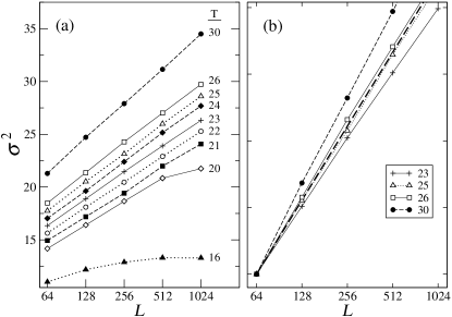
Figure 1: (a) Surface thickness $\sigma^{2}$ as a function of the log of lattice size $L$ for different temperatures $T$. (b) Expanded view of (a) for several temperatures near $T_{R}$ shifted vertically to coincide at $L=64$. Dashed line is the expected KT slope at $T_{R}$, showing that $T_{R}$ is slightly above $T=25$ but below 26.

Figure 1(a) shows simulation results for the scaling of the surface roughness $\sigma^{2}$ with the length $L$ of the lattice in simulations with different lattice sizes $L^{2}$ up to $1024^{2}$ and at several temperatures $T$ from 16 to 30. KT theory 73kos1181 ; 74kos1046 predicts a logarithmic divergence for $\sigma^{2}$ with a universal slope at $T_{R}$

$$\sigma^{2}(L)=\sigma_{0}^{2}(T_{R})+\frac{a^{2}}{\pi^{2}}\ln L,$$ (5)

where $a$ is the lattice constant of the surface, and in the units of Eqn.(4), $a=2\pi$. Therefore, at $T_{R}$ the slope of Fig. 1(a) should be equal to 4. Above $T_{R}$, the logarithmic behavior of $\sigma^{2}$ continues to hold except the constant $\sigma_{0}^{2}$ as well as the slope both increase with $T$. The data in Fig. 1(a) show that for $T=21$ and below, $\sigma^{2}$ appears to approach a finite value as $L\to\infty$. Therefore, it is clear that $T_{R}>21$. The most recent simulation of the SG model by Sanchez et al. 00san3219 (referred to as the “ordered SG model”, OSGM, in this paper) suggested that $T_{R}\approx 16$. Our data show that this is incorrect, and their error is likely due to slow sampling problems. Locating the precise value of $T_{R}$ is more involved, since the data for $T>21$ show no obvious tendency toward a finite $\sigma^{2}$. There are two possibilities: either these temperatures are above $T_{R}$ or the system size may not be large enough to have reached the scaling limit for these temperatures. To determine which one is the case, we must resort to a comparison between the simulation data with KT theory. Figure 1(b) shows an expanded view of Fig. 1(a) for a few temperatures $23<T<30$, but for each $T$ the curve has been shifted vertically to remove the offset $\sigma_{0}^{2}$ so that they all coincide at $L=64$. The heavy dashed line indicates the KT slope at $T_{R}$ according to Eqn.(5). The data therefore suggest that $T_{R}$ is slightly larger than 25 but less than 26, which is consistent with the RG prediction for $T_{R}=8\pi$ in the continuum model 80ami585 ; 80kno597 . The apparent lack of an asymptotic $\sigma^{2}$ in the data for $21<T<T_{R}$ implies that even for $L=1024$, these lattice sizes are not yet large enough to be in the scaling limit for those temperatures. Finally, to compare the dynamic scaling behavior of the switching algorithm with Metropolis, Fig. 2 shows the relaxation time in the measurement of $\sigma^{2}$ with the lattice size $L$ slightly above $T_{R}$. Compared with the dynamic exponent $\xi\approx 2.5$ in Metropolis, the switching algorithm shows a markedly improved $\xi\approx 1.4$.

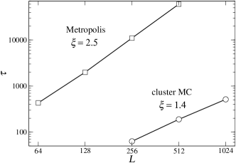
Figure 2: Dynamic scaling for the relaxation time $\tau$ (in units of MC passes) of $\sigma^{2}$ as a function of lattice size $L$ in Metropolis versus cluster MC, with their corresponding exponent $\xi$.

- (1) See, for example: K.E. Schmidt, Phys. Rev. Lett. 51, 2175 (1983); G.G. Batrouni, G.R. Katz, A.S. Kronfield, G.P. Lepage, B. Svetitsky and K.G. Wilson, Phys. Rev. D 32, 2736 (1985); E. Dagotto and J.B. Kogut, Phys. Rev. Lett. 58, 299 (1987); and J. Goodman and A.D. Sokal, Phys. Rev. Lett. 56, 1015 (1986).
- (2) R.H. Swendsen and J.-S. Wang, Phys. Rev. Lett. 58, 86 (1987).
- (3) R.G. Edwards and A.D. Sokal, Phys. Rev. D 38, 2009 (1988).
- (4) D. Kandel, E. Domany, D. Ron, A. Brandt and E. Loh, Phys. Rev. Lett. 60, 1591 (1988).
- (5) U. Wolff, Phys. Rev. Lett. 60, 1461 (1988).
- (6) F. Niedermayer, Phys. Rev. Lett. 61, 2026 (1988).
- (7) U. Wolff, Phys. Rev. Lett. 62, 361 (1989).
- (8) D. Kandel, R. Ben-Av and E. Domany, Phys. Rev. Lett. 65, 941 (1990).
- (9) J.S. Wang and R.H. Swendsen, Physica A 167, 565 (1990).
- (10) D. Kandel and E. Domany, Phys. Rev. B 43, 8539 (1991).
- (11) H.G. Evertz, M. Hasenbusch, M. Marcu, K. Pinn and S. Solomon, Phys. Lett. B 254, 185 (1991).
- (12) S. Liang, Phys. Rev. Lett. 69, 2145 (1992).
- (13) M. Hasenbusch, L. Gideon, M. Marcu and K. Pinn, Phys. Rev. B 46, 10472 (1992).
- (14) M. Hasenbusch, M. Marcu and K. Pinn, Physica A 211, 255 (1994).
- (15) C. Dress and W. Krauth, J. Phys. A 28, L597 (1995).
- (16) J. Houdayer, European Phys. J. B 22, 479 (2001).
- (17) H.W.J. Blote, J.R. Heringa and E. Luijten, Comp. Phys. Comm. 147, 58 (2002).
- (18) W. Krauth and R. Moessner, Phys. Rev. B 67, 064503 (2003).
- (19) J.W. Liu and E. Luijten, Phys. Rev. Lett. 92, 035504 (2004).
- (20) C.M. Fortuin and P.W. Kasteleyn, Physica 57, 536 (1972).
- (21) N. Metropolis, A.W. Rosenbluth, M.N. Rosenbluth, A.H. Teller and E. Teller, J. Chem. Phys. 21, 1087 (1953).
- (22) N. Metropolis and S. Ulam, J. Am. Stat. Assoc. 44, 335 (1949).
- (23) K. Binder, Monte Carlo Methods in Statistical Physics, Topics of Current Physics, Vol. 7, (Springer, Berlin, 1986).
- (24) C.H. Mak, J. Chem. Phys. 122, 214110 (2005).
- (25) S.T. Chui and J.D. Weeks, Phys. Rev. B 14, 4978 (1976).
- (26) J.M. Kosterlitz and D.J. Thouless, J. Phys. C 6, 1181 (1973).
- (27) J.M. Kosterlitz, J. Phys. C 7, 1046 (1974).
- (28) R.H. Swendsen, Phys. Rev. B 15, 5421 (1977).
- (29) W.J. Shugard, J.D. Weeks and G.H. Gilmer, Phys. Rev. Lett. 41, 1399 (1978).
- (30) F. Falo, A.R. Bishop, P.S. Lomdahl and B. Horovitz, Phys. Rev. B 43, 8081 (1991).
- (31) A. Sanchez, D. Cai, N. Gronbech-Jensen, A.R. Bishop and Z.J. Wang, Phys. Rev. B 51, 14664 (1995).
- (32) A. Sanchez, A.R. Bishop and E. Moro, Phys. Rev. E 62, 3219 (2000).
- (33) T. Nakayama, K. Yakubo and R.L. Orbach, Rev. Mod. Phys. 66, 381 (1994).
- (34) Y Hoffman and E. Ribak, Astrophys. J. 380, L5 (1991).
- (35) D.J. Amit, Y.Y. Goldschmidt and S. Grinstein, J. Phys. A 13, 585 (1980).
- (36) H.J.F. Knops and L.W.J. den Ouden, Physica A 103, 597 (1980).