An information-based traffic control in a public conveyance system:
reduced clustering and enhanced efficiency

Abstract

A new public conveyance model applicable to buses and trains is proposed in this paper by using stochastic cellular automaton. We have found the optimal density of vehicles, at which the average velocity becomes maximum, significantly depends on the number of stops and passengers behavior of getting on a vehicle at stops. The efficiency of the hail-and-ride system is also discussed by comparing the different behavior of passengers. Moreover, we have found that a big cluster of vehicles is divided into small clusters, by incorporating information of the number of vehicles between successive stops.

I INTRODUCTION

The totally asymmetric simple exclusion process sz ; derrida ; schuetz is the simplest model of non-equilibrium systems of interacting self-driven particles. Various extensions of this model have been reported in the last few years for capturing the essential features of the collective spatio-temporal organizations in wide varieties of systems, including those in vehicular traffic css ; helbing ; Schad ; nagatanirev ; cnss . Traffic of buses and bicycles have also been modeled following similar approaches oloan ; jiang . A simple bus route model oloan exhibits clustering of the buses along the route and the quantitative features of the coarsening of the clusters have strong similarities with coarsening phenomena in many other physical systems. Under normal circumstances, such clustering of buses is undesirable in any real bus route as the efficiency of the transport system is adversely affected by clustering. The main aim of this paper is to introduce a traffic control system into the bus route model in such a way that helps in suppressing this tendency of clustering of the buses. This new model exhibits a competition between the two opposing tendencies of clustering and de-clustering which is interesting from the point of view of fundamental physical principles. However, the model may also find application in developing adaptive traffic control systems for public conveyance systems.

In some of earlier bus-route models, movement of the buses was monitored on coarse time intervals so that the details of the dynamics of the buses in between two successive bus stops was not described explicitly. Instead, the movement of the bus from one stop to the next was captured only through probabilities of hopping from one stop to the next; hopping takes place with the lower probability if passengers are waiting at the approaching bus stop oloan . An alternative interpretation of the model is as follows: the passengers could board the bus whenever and wherever they stopped a bus by raising their hand, this is called the hail-and-ride system.

Several possible extensions of the bus route model have been reported in the past cd ; nagatani ; Chi . For example, in cd , in order to elucidate the connection between the bus route model with parallel updating and the Nagel-Schreckenberg model, two alternative extensions of the latter model with space-/time-dependent hopping rates are proposed. If a bus does not stop at a bus stop, the waiting passengers have to wait further for the next bus; such scenarios were captured in one of the earlier bus route models nagatani , using modified car-following model. In Chi , the bus capacity, as well as the number of passengers getting on and off at each stop, were introduced to make the model more realistic. Interestingly, it has been claimed that the distribution of the time gaps between the arrival of successive buses is described well by the Gaussian Unitary Ensemble of random matrices Mex .

In this paper, by extending the model in oloan , we suggest a new public conveyance model (PCM). Although we refer to each of the public vehicles in this model as a “bus”, the model is equally applicable to train traffic on a given route. In this PCM we can set up arbitrary number of bus stops on the given route. The hail-and-ride system turns out to be a special case of the general PCM. Moreover, in the PCM the duration of the halt of a bus at any arbitrary bus stop depends on the number of waiting passengers. As we shall demonstrate in this paper, the delay in the departure of the buses from crowded bus stops leads to the tendency of the buses to cluster on the route. Furthermore, in the PCM, we also introduce a traffic control system that exploits the information on the number of buses in the “segments” in between successive bus stops; this traffic control system helps in reducing the undesirable tendency of clustering by dispersing the buses more or less uniformly along the route.

In this study we introduce two different quantitative measures of the efficiency of the bus transport system, and calculate these quantities, both numerically and analytically, to determine the conditions under which the system would operate optimally.

This paper is organized as follows, in Sec. $2$ PCM is introduced and we show several simulation results in Sec. $3$. The average speed and the number of waiting passengers are studied by mean field analysis in Sec. $4$, and conclusions are given in Sec. $5$.

II A STOCHASTIC CA MODEL FOR PUBLIC CONVEYANCE

In this section, we explain the PCM in detail. For the sake of simplicity, we impose periodic boundary conditions. Let us imagine that the road is partitioned into $L$ identical cells such that each cell can accommodate at most one bus at a time. Moreover, a total of $S$ ($0\leq S\leq L$) equispaced cells are identified in the beginning as bus stops. Note that, the special case $S=L$ corresponds to the hail-and-ride system. At any given time step, a passenger arrives with probability $f$ to the system. Here, we assume that a given passenger is equally likely to arrive at any one of the bus stops with a probability $1/S$. Thus, the average number of passengers that arrive at each bus stop per unit time is given by $f/S$. In contrast to this model, in ref. cgns ; kjnsc the passengers were assumed to arrive with probability $f$ at all the bus stops in every time step.

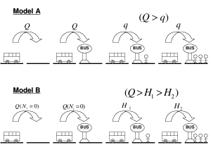
Figure 1: Schematic illustration of the PCM. In the model A, the hopping probability to the bus stop does not depend on the number of waiting passengers. In contrast, in the model B the hopping probability to the bus stop depends on the number of waiting passengers. Thus if the waiting passengers increase, the hopping probability to the bus stop is decreased.

The model A corresponds to those situations where, because of sufficiently large number of broad doors, the time interval during which the doors of the bus remain open after halting at a stop, is independent of the size of waiting crowd of passengers. In contrast, the model B captures those situations where a bus has to halt for a longer period to pick up a larger crowd of waiting passengers.

The symbol $H$ is used to denote the hopping probability of a bus entering into a cell that has been designated as a bus stop. We consider two different forms of $H$ in the two versions of our model which are named as model A and model B. In the model A we assume the form

$$H=\left\{\begin{array}[]{cl}Q&{\rm\,\,\,\,\,\,no\,\,waiting\,\,passengers}\\ q&{\rm\,\,\,\,\,\,waiting\,\,passengers\,\,exist}\end{array}\right.$$ (1)

where both $Q$ and $q$ ($Q>q$) are constants independent of the number of waiting passengers. The form (1) was used in the original formulation of the bus route model by O’Loan et al. oloan .

In contrast to most of all the earlier bus route models, we assume in the model B that the maximum number of passengers that can get into one bus at a bus stop is $N_{\rm max}$. Suppose, $N_{i}$ denotes the number of passengers waiting at the bus stop $i$ $(i=1,\cdots,S)$ at the instant of time when a bus arrives there. In contrast to the form (1) for $H$ in model A, we assume in model B the form

$$H=\frac{Q}{\min(N_{i},N_{\rm max})+1}$$ (2)

where $\min(N_{i},N_{\rm max})$ is the number of passengers who can get into a bus which arrives at the bus stop $i$ at the instant of time when the number of passengers waiting there is $N_{i}$. The form (2) is motivated by the common expectation that the time needed for the passengers boarding a bus is proportional to their number. FIG. 1 depicts the hopping probabilities in the two models A and B schematically.

The hopping probability of a bus to the cells that are not designated as bus stops is $Q$; this is already captured by the expressions (1) and (2) since no passenger ever waits at those locations.

In principle, the hopping probability $H$ for a real bus would depend also on the number of passengers who get off at the bus stop; in the extreme situations where no passenger waits at a bus stop the hopping probability $H$ would be solely decided by the disembarking passengers. However, in order to keep the model theoretically simple and tractable, we ignore the latter situation and assume that passengers get off only at those stops where waiting passengers get into the bus and that the time taken by the waiting passengers to get into the bus is always adequate for the disembarking passengers to get off the bus.

Note that $N_{\rm max}$ is the maximum boarding capacity at each bus stop rather than the maximum carrying capacity of each bus. The PCM model reported here can be easily extended to incorporate an additional dynamical variable associated with each bus to account for the instantaneous number of passengers in it. But, for the sake of simplicity, such an extension of the model is not reported here. Instead, in the simple version of the PCM model reported here, $N_{\rm max}$ can be interpreted as the maximum carrying capacity of each bus if we assume that all of the passengers on the bus get off whenever it stops.

The model is updated according to the following rules. In step $2-4$, these rules are applied in parallel to all buses and passengers, respectively:

1. Arrival of a passenger
   A bus stop $i$ ($i=1,\cdots,S$) is picked up randomly, with probability $1/S$, and then the corresponding number of waiting passengers in increased by unity, i.e. $N_{i}$ $\rightarrow$ $N_{i}+1$, with probability $f$ to account for the arrival of a passenger at the selected bus stop.

2. Bus motion
   If the cell in front of a bus is not occupied by another bus, each bus hops to the next cell with the probability $H$. Specifically, if passengers do not exist in the next cell in both model A and model B hopping probability equals to $Q$ because $N_{i}$ equals to 0. Else, if passengers exist in the next cell, the hopping probability equals to $q$ in the model A, whereas in the model B the corresponding hopping probability equals to $Q/(\min(N_{i},N_{\rm max})+1)$. Note that, when a bus is loaded with passengers to its maximum boarding capacity $N_{\rm max}$, the hopping probability in the model B equals to $Q/(N_{\rm max}+1)$, the smallest allowed hopping probability.

3. Boarding a bus
   When a bus arrives at the $i$-th ($i=1,\cdots,S$) bus stop cell, the corresponding number $N_{i}$ of waiting passengers is updated to $\max(N_{i}-N_{\rm max},0)$ to account for the passengers boarding the bus. Once the door is closed, no more waiting passenger can get into the bus at the same bus stop although the bus may remain stranded at the same stop for a longer period of time either because of the unavailability of the next bus stop or because of the traffic control rule explained next.

4. Bus information update
   Every bus stop has information $I_{j}$ ($j=1,\cdots,S$) which is the number of buses in the segment of the route between the stop $j$ and the next stop $j+1$ at that instant of time. This information is updated at each time steps. When one bus leaves the $j$-th bus stop, $I_{j}$ is increased to $I_{j}+1$. On the other hand, when a bus leaves $(j+1)$-th bus stop, $I_{j}$ is reduced to $I_{j}-1$. The desirable value of $I_{j}$ is $I_{0}=m/S$, where $m$ is the total number of buses, for all $j$ so that buses are not clustered in any segment of the route. We implement a traffic control rule based on the information $I_{j}$: a bus remains stranded at a stop $j$ as long as $I_{j}$ exceeds $I_{0}$.

We use the average speed $\langle V\rangle$ of the buses and the number of the waiting passengers $\langle N\rangle$ at a bus stop as two quantitative measures of the efficiency of the public conveyance system under consideration; a higher $\langle V\rangle$ and smaller $\langle N\rangle$ correspond to an efficient transportation system.

III COMPUTER SIMULATIONS OF PCM

In the simulations we set $L=500,Q=0.9,q=0.5$ and $N_{\rm max}=60$. The main parameters of this model, which we varied, are the number of buses ($m$), the number of bus stops ($S$) and the probability ($f$) of arrival of passengers. The number density of buses is defined by $\rho=m/L$.

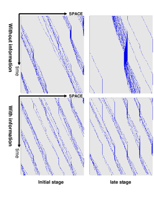
Figure 2: Space-time plots in the model B for the parameter values $f=0.6,S=5,m=30$. The upper two figures correspond to the case where no traffic control system based on the information $\{I\}$ is operational. The upper left figure corresponds to the initial stage (from $t=1000$ to $t=1500$) whereas the upper right plot corresponds to the late stages (from $t=4000$ to $t=4500$). The lower figures correspond to the case where the information ($\{I\}$) based bus-traffic control system is operational (left figure shows data from $t=1000$ to $t=1500$ while the right figure corresponds to $t=4000$ to $t=4500$). Clearly, information-based traffic control system disperses the buses which, in the absence of this control system, would have a tendency to cluster.

Typical space-time plots of the model B are given in FIG. 2. If no information-based traffic control system exits, the buses have a tendency to cluster; this phenomenon is very simular to that observed in the ant-trail model cgns ; kjnsc . However, implementation of the information-based traffic control system restricts the size of such clusters to a maximum of $I_{0}$ buses in a segment of the route in between two successive bus stops. We study the effects of this control system below by comparing the characteristics of two traffic systems one of which includes the information-based control system while the other does not.

III.1 PCM without information-based traffic control

In the FIG. 3 - FIG. 8, we plot $\langle V\rangle$ and $\langle N\rangle$ against the density of buses for several different values of $f$. Note that, the FIG. 5 and FIG. 8 corresponds to the hail-and-ride system for models A and B, respectively.

Figure 3: The average speed and the average number of waiting passengers in the model A are plotted against the density for the parameters $S=5$ and $f=0.3$, 0.6 and 0.9.

Figure 4: The plot of $\langle V\rangle$ and $\langle N\rangle$ of the model A for $S=50$ and $f=0.3$, 0.6 and 0.9.

Figure 5: The plot of $\langle V\rangle$ and $\langle N\rangle$ of the model A for $S=500(=L)$ and $f=0.3$, 0.6 and 0.9.

Figure 6: The plot of $\langle V\rangle$ and $\langle N\rangle$ of the model B for $S=5$ and $f=0.3$, 0.6 and 0.9.

Figure 7: The plot of $\langle V\rangle$ and $\langle N\rangle$ of the model B for $S=50$ and $f=0.3$, 0.6 and 0.9.

Figure 8: The plot of $\langle V\rangle$ and $\langle N\rangle$ of the model B for $S=500(=L)$ and $f=0.3$, 0.6 and 0.9.

Figure 9: The distribution of waiting passengers is plotted against all bus stops for the parameters $f=0.6$, $B=50$, $S=50$. The horizontal line means the ranking, where we arrange the bus stops according to the descending order of $\langle N\rangle$.

Figure 10: The average speed and the average number of waiting passengers in the model B are plotted against the density for the parameters $f=0.9,S=50$; the hopping parameters are $Q=0.8$ and $Q=1.0$.

Figure 11: The optimal density of buses in the model B is plotted against $Q$. The parameters are $f=0.9,S=5$ (normal line),$f=0.6,S=5$ (finer broken line), $f=0.9,S=50$ (bold broken line), $f=0.6,S=50$ (longer broken line).

Figure 12: Comparison between the case of bus capacity $60$ with bus capacity $120$. The parameters are $Q=0.9$, $S=10$, $f=0.6$ in the model B without information. The top figure shows the average velocity, the center figure shows waiting passengers and the bottom figure shows the number of conveyed passengers per unit bus, i.e. this number is calculated by (total number of on-boarding passengers on all buses)/(the number of buses), against the bus density up to $0.5$. In each figure, the horizontal axis shows the density; the numbers without parentheses denote the number densities in the case $N_{\rm max}=60$, whereas the numbers in the parentheses denote the number densities in the case $N_{\rm max}=120$.

These figures demonstrate that the average speed $\langle V\rangle$, which is a measure of the efficiency of the bus traffic system, exhibits a maximum at around $\rho=0.2\sim 0.3$ especially in the model B (comparing FIG. 3 with FIG. 6, it shows the model B (FIG. 6) reflects the bus bunching more clearly than the model A (FIG. 3) especially at large f and small $\rho$). The average number of waiting passengers $\langle N\rangle$, whose inverse is another measure of the efficiency of the bus traffic system, is vanishingly small in the region $0.3<\rho<0.7$; $\langle N\rangle$ increases with decreasing (increasing) $\rho$ in the regime $\rho<0.3$ ($\rho>0.7$).

The average velocity of the model A becomes smaller as S increases in the low density region (see FIG. 3, FIG. 4 and FIG. 5). In contrast, in the model B (FIG. 7 and FIG. 8) we observe that there is no significant difference in the average velocity. Note that the number of waiting passengers is calculated by (total waiting passengers)/(number of bus stops). The total number of waiting passengers in this system is almost the same under the case $S=50$ and hail-and-ride system $S=L$ in both models. When the parameter $S$ is small (comparing FIG. 3 and FIG. 6), in the model B the waiting passengers are larger and the average velocity is smaller than in the model A, since the effect of the delay in getting on a bus is taken into account. In the model B (comparing FIG. 6, FIG. 7 and FIG. 8), the case $S=50$ is more efficient than $S=5$, i.e. the system is likely to become more efficient, as $S$ increases. However, we do not find any significant variation between $S=50$ and $S=500$. When $S$ is small, the system becomes more efficient by increasing the number of bus stops. If the number of bus stops increase beyond $50$, then there is little further variation of the efficiency as $S$ is increased up to the maximum value $500$.

From FIG. 9, the distribution of $\langle N\rangle$ over all the bus stops in the system is shown. We see that the distribution does not show the Zipf’s law, which is sometimes seen in natural and social phenomena; frequency of used words word , population of a city population , the number of the access to a web site web , and intervals between successive transit times of the cars of traffic flow musha .

Next, we investigate the optimal density of buses at which the average velocity becomes maximum. The optimal density depends on $Q$ and is $\rho=0.3$ for $Q=0.8$ (FIG. 10, see also FIG. 11). In FIG. 10, it is shown that the density corresponding to the maximum velocity shifts to higher values as $Q$ becomes larger. FIG. 11 shows the optimal density of buses in the model B without information-based control system. From this figure, we find that the optimal density, for case $S=50$, is smaller than that for $S=5$. Moreover, for given $S$, the optimal density decreases with decreasing $f$. However, for both $S=5$ and $S=50$, the optimal density corresponding to $Q=1.0$ is higher for $f=0.6$ than that for $f=0.9$.

What is more effective way of increasing the efficiency of the public conveyance system on a given route by increasing the number of buses without increasing the carrying capacity of each bus, or by increasing the carrying capacity of each bus without recruiting more buses? Or, are these two prescriptions for enhancing efficiency of the public conveyance system equally effective? In order to address these questions, we make a comparative study of two situations on the same route: for example, in the first situation the number of buses is $10$ and each has a capacity of $60$, whereas in the second the number of buses is $5$ and each has a capacity of $120$. Note that the total carrying capacity of all the buses together is $600$ ($60\times 10$ and $120\times 5$ in the two situations), i.e., same in both the situations. But, the number density of the buses in the second situation is just half of that in the first as the length of the bus route is same in both the situations. In FIG. 12, the results for these two cases are plotted; the different scales of density used along the $X$-axis arises from the differences in the number densities mentioned above.

From FIG. 12, we conclude that, at sufficiently low densities, the average velocity is higher for $N_{\rm max}=60$ compared to those for $N_{\rm max}=120$. But, in the same regime of the number density of buses, larger number of passengers wait at bus stops when the bus capacity is smaller. Thus, in the region $\rho<0.05$, system administrators face a dilemma: if they give priority to the average velocity and decide to choose buses with $N_{\rm max}=60$, the number of passengers waiting at the bus stops increases. On the other hand if they decide to make the passengers happy by reducing their waiting time at the bus stops and, therefore, choose buses with $N_{\rm max}=120$, the travel time of the passengers after boarding a bus becomes longer.

However, at densities $\rho>0.05$, the system administrators can satisfy both the criteria, namely, fewer waiting passengers and shorter travel times, by one single choice. In this region of density, the public conveyance system with $N_{\rm max}=60$ is more efficient than that with $N_{\rm max}=120$ because the average velocity is higher and the number of waiting passengers is smaller for $N_{\rm max}=60$ than for $N_{\rm max}=120$. Thus, in this regime of bus density, efficiency of the system is enhanced by reducing the capacity of individual buses and increasing their number on the same bus route.

Figure 13: The plot of $\langle V\rangle$ and $\langle N\rangle$ of the model B with information ($S=5$ and $f=0.3$, 0.6 and 0.9)

Figure 14: The model B with $S=5$ and $f=0.9$. The left vertical dash line is $\rho=0.28$ and the right is $\rho=0.73$ in the two figures.

III.2 PCM with information-based traffic control

The results for the PCM with information-based traffic control system is shown in FIG. 13 and FIG. 14. In the FIG. 13 we plot $\langle V\rangle$ and $\langle N\rangle$ against the density of buses for the parameter $S=5$. The density corresponding to the peak of the average velocity shifts to lower values when the information-based traffic control system is switched on.

The data shown in FIG. 14 establish that implementation of the information-based traffic control system does not necessarily always improve the efficiency of the public conveyance system. In fact, in the region $0.3<\rho<0.7$, the average velocity of the buses is higher if the information-based control system is switched off. Comparing $\langle V\rangle$ and $\langle N\rangle$ in FIG. 14, we find that information-based traffic control system can improves the efficiency by reducing the crowd of waiting passengers. But, in the absence of waiting passengers, introduction of the information-based control system adversely affects the efficiency of the public conveyance system by holding up the buses at bus stops when the number of buses in the next segment of the route exceeds $I_{0}$.

Figure 15: Distribution of headway distance for $S=10$, $m=50$, $f=0.9$ in model B. This figure shows the plot of headway distance against the ranking.

Finally, FIG. 15 shows the distribution of headway distance against the ranking, where we arrange the order of magnitude according to the headway distance of buses in descending order. From this figure it is found that the headway distribution is dispersed by the effect of the information. The average headway distance with the information-based traffic control is equal to $8.34$, in contrast to a much shorter value of $0.66$ when that control system is switched off. Thus we confirm that the availability of the information $I_{j}$ and implementation of the traffic control system based on this information, significantly reduces the undesirable clustering of buses.

IV MEAN FIELD ANALYSIS

Let us estimate $\langle V\rangle$ theoretically in the low density limit $\rho\to 0$. Suppose, $T$ is the average time taken by a bus to complete one circuit of the route. In the model A, the number of hops made by a bus with probability $q$ during the time $T$ is $S$, i.e. the total number of bus stops. Therefore the average period $T$ for a bus in the model A is well approximated by

$$T=\frac{L-S}{Q}+\frac{S}{q}$$ (3)

and hence,

$$\langle V\rangle=\frac{L}{T}=\frac{LQq}{q(L-S)+QS}\,.$$ (4)

In model B, in the low density limit where $m$ buses run practically unhindered and are distributed uniformly in the system without correlations, the average number of passengers $N$ waiting at a bus stop, just before the arrival of the next bus, is

$$N=\frac{f}{S}\left(\frac{\frac{L}{S}-1}{Q}+\frac{1}{q}\right)\frac{S}{m}.$$ (5)

The first factor $f/S$ on the right hand side of the equation (5) is the probability of arrival of passengers per unit time. The second factor on the right hand side of (5) is an estimate of the average time taken by a bus to traverse one segment of the route, i.e. the part of the route between successive bus stops. The last factor in the same equation is the average number of segments of the route in between two successive buses on the same route. Instead of the constant $q$ used in (4) for the evaluation of $\langle V\rangle$ in the model A, we use

$$\bar{q}=\frac{Q}{N+1}$$ (6)

in eq. (4) and eq. (5) for the model B. Then, for the model B, the hopping probability $Q$ is estimated self-consistently solving

$$\langle V\rangle=Q-\frac{f}{m},$$ (7)

(4) and (6) simultaneously.

We also obtain, for the model B, the average number of passengers $\langle N\rangle$ waiting at a bus stop in the $\rho\to 0$ limit. The average time for moving from one bus stop to the next is $\Delta t=(L/S-1)/Q+1/{\bar{q}}$ and, therefore, we have

$$\langle N\rangle = (f/S)\cdot(\Delta t+2\Delta t+\cdots+(S-1)\Delta t)/S$$ (8)

$$= \frac{f(S-1)({\bar{q}}(L-S)+SQ)}{2S^{2}Q{\bar{q}}}.$$

As long as the number of waiting passengers does not exceed $N_{\rm max}$, we have observed reasonably good agreement between the analytical estimates (4), (8) and the corresponding numerical data obtained from computer simulations. For example, in the model A, we get the estimates $\langle V\rangle=0.85$ and $\langle N\rangle=1.71$ from the approximate mean field theory for the parameter set $S=50$, $m=1$, $Q=0.9$, $q=0.5$, $f=0.3$. The corresponding numbers obtained from direct computer simulations of the model A version of PCM are 0.84 and 1.78, respectively. Similarly, in the model B under the same conditions, we get $\langle V\rangle=0.60$ and $\langle N\rangle=2.45$ from the mean field theory, while the corresponding numerical values are 0.60 and 2.51, respectively. If we take sufficiently small $f$’s, then the mean-field estimates agree almost perfectly with the corresponding simulation data. However, our mean field analysis breaks down when a bus can not pick up all the passengers waiting at a bus stop.

V CONCLUDING DISCUSSIONS

In this paper, we have proposed a public conveyance model (PCM) by using stochastic CA. In our PCM, some realistic elements are introduced: e.g., the carrying capacity of a bus, the arbitrary number of bus stops, the halt time of a bus that depends on the number of waiting passengers, and an information-based bus traffic control system which reduces clustering of the buses on the given route.

We have obtained quantitative results by using both computer simulations and analytical calculations. In particular, we have introduced two different quantitative measures of the efficiency of the public conveyance system. We have found that the bus system works efficiently in a region of moderate number density of buses; too many or too few buses drastically reduce the efficiency of the bus-transport system. If the density of the buses is lower than optimal, not only large number of passengers are kept waiting at the stops for longer duration, but also the passengers in the buses get a slow ride as buses run slowly because they are slowed down at each stop to pick up the waiting passengers. On the other hand, if the density of the buses is higher than optimal, the mutual hindrance created by the buses in the overcrowded route also lowers the efficiency of the transport system. Moreover, we have found that the average velocity increases, and the number of waiting passengers decreases, when the information-based bus traffic control system is switched on. However, this enhancement of efficiency of the conveyance system takes place only over a particular range of density; the information-based bus traffic control system does not necessarily improve the efficiency of the system in all possible situations.

We have compared two situations where the second situation is obtained from the first one by doubling the carrying capacity of each bus and reducing their number to half the original number on the same route. In the density region $\rho>0.05$ the system of $N_{\rm max}=60$ is more efficient than that with $N_{\rm max}=120$. However, at small densities ($\rho<0.05$), although the average velocity increases, the number of waiting passengers also increases, by doubling the carrying capacity from $N_{\rm max}=60$ to $N_{\rm max}=120$. Hence, bus-transport system administrators would face a dilemma in this region of small density.

Finally, in our PCM, the effect of the disembarking passengers on the halt time of the buses has not been captured explicitly. Moreover, this study is restricted to periodic boundary conditions. The clustering of particles occurs not only in a ring-like bus route, but also in shuttle services of buses and trains. Thus it would be interesting to investigate the effects of the information-based traffic control system also on such public transport systems. In a future work, we intend to report the results of our investigations of the model under non-periodic boundary conditions. We hope our model will help in understanding the mechanism of congestion in public conveyance system and will provide insight as to the possible ways to reduce undesirable clustering of the vehicles.

Acknowledgments: Work of one of the authors (DC) has been supported, in part, by the Council of Scientific and Industrial Research (CSIR), government of India.

References

- (1) B. Schmittmann and R.K.P. Zia, in: Phase Transition and Critical Phenomena, Vol. 17, eds. C. Domb and J. L. Lebowitz (Academic Press, 1995).
- (2) B. Derrida, Phys. Rep. 301, 65 (1998).
- (3) G. M. Schütz, in Phase Transitions and Critical Phenomena, vol. 19 (Acad. Press, 2001).
- (4) D. Chowdhury, L. Santen and A. Schadschneider, Phys. Rep. 329, 199 (2000).
- (5) D. Helbing, Rev. Mod. Phys. 73, 1067 (2001).
- (6) A. Schadschneider, Physica A 313, 153 (2002).
- (7) T. Nagatani, Rep. Prog. Phys. 65, 1331 (2002).
- (8) D. Chowdhury, K. Nishinari, L. Santen and A. Schadschneider, Stochastic Transport in Complex Systems, Elsevier (2008).
- (9) R. Jiang, B. Jia and Q. S. Wu, J. Phys. A: Math. Gen. 37, 2063 (2004)
- (10) O.J. O’Loan, M.R. Evans and M.E. Cates, Phys. Rev. E 58, 1404 (1998).
- (11) D. Chowdhury and R.C. Desai, Eur. Phys. J. B 15, 375 (2000).
- (12) T. Nagatani, Physica A 287, 302 (2000); Phys. Rev. E 63, 036115 (2001); Physica A 297, 260 (2001).
- (13) R. Jiang, M-B. Hu, B. Jia, and Q-S. Wu, Eur. Phys. J. B 34, 367 (2003).
- (14) M. Krbalek and P. Seba, J. Phys. A: Math. Gen. 33, L229 (2000).
- (15) D. Chowdhury, V. Guttal, K. Nishinari and A. Schadschneider, J. Phys. A: Math. Gen. 35, L573 (2002).
- (16) A. Kunwar, A. John, K. Nishinari, A. Schadschneider and D. Chowdhury, J. Phys. Soc. Jpn. 73, 2979 (2004).
- (17) G. K. Zipf: Human Behavior and the Principle of Least Effort, Addison-Wesley, Cambridge, 1949.
- (18) Y. M. Ioannides and H. G. Overman, Regional Science and Urban Economics, 33, 127 (2003).
- (19) M. E. J. Newman and D. J. Watts, Phys. Rev. E 60, 7332 (1999): M. E. J. Newman and D. J. Watts, Physics. Letters. A 263, 341 (1999).
- (20) T. Musha and H. Higuchi, Jpn. J. App. Phys. 15, 1271 (1976).