Magnetic exponents of two-dimensional Ising spin glasses

Abstract

The magnetic critical properties of two-dimensional Ising spin glasses are controversial. Using exact ground state determination, we extract the properties of clusters flipped when increasing continuously a uniform field. We show that these clusters have many holes but otherwise have statistical properties similar to those of zero-field droplets. A detailed analysis gives for the magnetization exponent $\delta\approx 1.30\pm 0.02$ using lattice sizes up to $80\times 80$; this is compatible with the droplet model prediction $\delta=1.282$. The reason for previous disagreements stems from the need to analyze both singular and analytic contributions in the low-field regime.

Spin glasses Mézard et al. (1987); Young (1998) have been the focus of much interest because of their many remarkable features: they undergo a subtle freezing transition as temperature is lowered, their relaxational dynamics is slow (non-Arrhenius), they exhibit ageing, memory effects, etc. Although there are still some heated disputes concerning three-dimensional spin glasses, the case of two dimensions is relatively consensual, at least in the absence of a magnetic field. Indeed, two recent studies Katzgraber et al. (2004); Hartmann and Houdayer (2004) found that the thermal properties of two-dimensional Ising spin glasses with Gaussian couplings agreed very well with the predictions of the scaling/droplet pictures Bray and Moore (1986); Fisher and Huse (1986). Interestingly, the situation in the presence of a magnetic field remains unclear; in particular, some Monte Carlo simulations Kinzel and Binder (1983) and basically all ground state studies Kawashima and Suzuki (1992); Barahona (1994); Rieger et al. (1996) seem to go against the scaling/droplet pictures. Nevertheless, since spin glasses often have large corrections to scaling, the apparent disagreement with the droplet picture resulting from these studies may be misleading and tests in one dimension give credence to this claim Carter et al. (2003).

In this study we use state of the art algorithms for determining exact ground states in the presence of a magnetic field and treat significantly larger lattice sizes than in previous work. By finding the precise points where the ground states change as a function of the field, we extract the excitations relevant in the presence of a field which can then be compared to the zero-field droplets. Although for small size lattices we agree with previous studies, at our larger ones a careful analysis, taking into account both the analytic and the singular terms, gives excellent agreement with the droplet picture.

The model and its properties —

We work on an $L\times L$ square lattice having Ising spins on its sites and couplings $J_{ij}$ on its bonds. The Hamiltonian is

$$H(\{\sigma_{i}\})\equiv-\sum_{\langle ij\rangle}J_{ij}\sigma_{i}\sigma_{j}-B\sum_{i}\sigma_{i}$$ (1)

The first sum runs over all nearest neighbor sites using periodic boundary conditions to minimize finite size effects. The $J_{ij}$ are independent random variables of either Gaussian or exponential distribution.

It is generally agreed that two-dimensional spin glasses have a unique critical point at $T=B=0$. There, the free energy is non-analytic and in fact, standard arguments Cardy (1996) suggest that as $T\to 0$ and $B\to 0$ the free energy goes as $\beta F(L,\beta)\sim\beta E_{0}+G_{s}(TL^{y_{T}},BL^{y_{B}})$ where $E_{0}$ is the ground-state energy, $\beta$ the inverse temperature, while $y_{T}$ and $y_{B}$ are the thermal and magnetic exponents. Previous work when $B=0$ is compatible with this form and in fact also agrees with the scaling/droplet picture of Ising spin glasses in which one has $y_{T}=-\theta\approx 0.282$. The stumbling block concerns the behavior when $B\neq 0$; there, the droplet prediction in general dimension $d$ is

$$y_{B}=y_{T}+d/2$$ (2)

but the numerical evidence for this is muddled at best. It is thus worth reviewing the hypotheses assumed by the droplet model so that they can be tested directly.

We begin with the fact that in any dimension $d$, a magnetic field destabilizes the ground state beyond a characteristic length scale $\xi_{B}$. To see this, consider an infinitesimal field and zero-field droplets of scale $\ell$. These are expected to be compact. The interfacial energy of such droplets is $O(\ell^{\theta})$ while their total magnetization goes as $\ell^{d/2}$. The magnetic and interfacial energy are then balanced when $B$ reaches a value $O(1/\ell^{d/2-\theta})$: at that value of the field, some of the droplets will flip and the ground state will be destabilized. We then see that for each field strength there is an associated magnetic length scale $\xi_{B}$

$$\xi_{B}\approx B^{-\frac{1}{{\frac{d}{2}-\theta}}}$$ (3)

This leads to the identification $y_{B}=d/2-\theta$ in agreement with Eq. 2, giving $y_{b}\approx 1.282$ at $d=2$.

The droplet model also predicts the scaling of the magnetization in the $B\to 0$ limit via the exponent $\delta$:

$$m(B)\sim B^{1/\delta}$$ (4)

If this form also holds for infinitesimal fields at finite $L$, we can consider the field $B^{*}$ for which system-size droplets flip; this happens when $B=O(1/L^{y_{B}})$ and then the magnetization is $O(L^{-d/2})$, the droplets having random magnetizations. This leads to $m(B^{*})\sim L^{-d/2}$ and $m(B^{*})\sim[1/L^{y_{B}}]^{1/\delta}$ so that

$$d\delta=2y_{B}$$ (5)

Although the droplet model arguments are not proofs, they seem quite convincing. Nevertheless, the numerical studies measuring $\delta$ do not give good agreement with the prediction $\delta=1.282$. For instance, using Monte Carlo at “low enough” temperatures, Kinzel and Binder Kinzel and Binder (1983) find $\delta\approx 1.39$. Since thermalization is difficult at low temperatures, it is preferable to work directly with ground states, at least when that is possible. This was done by three independent groups Kawashima and Suzuki (1992); Barahona (1994); Rieger et al. (1996) with increasing power, leading to $\delta\approx 1.48$, $\delta\approx 1.54$ and $\delta\approx 1.48$. Taken together, these studies show a real discrepancy with the droplet prediction. To save the droplet model from this thorny situation, one can appeal to large corrections to scaling. Such potential effects have been considered Carter et al. (2003) in dimension one where it was shown that $\xi_{B}$ was poorly fitted by a pure power law unless the fields were very small. Here we revisit the two-dimensional case to reveal either the size of the corrections to scaling or a cause for the break down of the droplet reasoning.

Computation of ground states —

We determine the exact ground state of the Hamiltonian (1) by computing a maximum cut in the graph of interactions Barahona (1982), a prominent problem in combinatorial optimization. Whereas it is polynomially solvable on two-dimensional grids without a field and couplings bounded by a polynomial in the size of the input, it is NP-hard with an external field. In practice, we rely on a branch-and-cut algorithm Barahona et al. (1988); Liers et al. (2004).

Let the ground state at a field $B$ be denoted as $\{\sigma^{(G)}(B)\}$. To study the magnetization, we computed the ground states at increasing values of $B$, in steps of size $0.02$. When focusing instead on the flipping clusters, we had to determine the intervals in which the ground state was constant and in what manner it changed when going from one interval to the next. In Fig. 1 we show the associated piecewise constant magnetization curves for three samples of the disorder variables $J_{ij}$ at $L=10$.

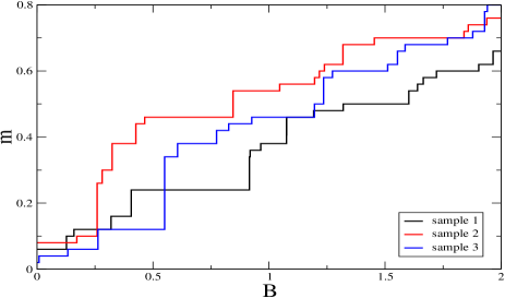
Figure 1: Magnetization as a function of $B$ for three typical $L=10$ samples.

To get the sequence of intervals or break points associated with such a function exactly, we start by computing the ground state in zero field. By applying postoptimality analysis from linear programming theory, we determine Rieger et al. (1996); Liers et al. (2004) a range $\Delta B$ such that the ground state at a field $B$ remains the optimum in the interval $[B,B+\Delta B]$. We reoptimize at $B+\Delta B+\epsilon$, with $\epsilon$ being a sufficiently small number. By repeatedly applying this procedure, we get a new ground state configuration, and increase $B$ until all spins are aligned with the field. This procedure works for system sizes in which the branch-and-cut program can prove optimality without branching, i.e., without dividing the problem into smaller sub-problems. If the algorithm branches (this occurs only for the largest system sizes studied here), we apply a divide-and-conquer strategy for determining $\{\sigma^{(G)}(B)\}$ in an interval, say $[B_{1},B_{2}]$. For a fixed configuration the Hamiltonian (1) is linear in the field, the slope being the system’s magnetization. Let $f_{1},f_{2}$ be the two linear functions associated with $\{\sigma^{(G)}(B_{1})\}$ and $\{\sigma^{(G)}(B_{2})\}$. If $f_{1}$ and $f_{2}$ are equal, we are done. Otherwise, we determine the field $B_{3}$ at which the functions intersect and recursively solve the problem in the intervals $[B_{1},B_{3}]$ and $[B_{3},B_{2}]$.

A typical sample at $L=80$ requires about 2 hours of cpu on a work station for determining the ground states when $B$ goes through the multiples of $0.02$. The more time consuming computation of the exact break points takes about 4 hours on typical samples with $L=60$, but less than a minute if $L\leq 30$ because the ground-state determinations are fast and branching almost never arises. For our work, we considered mainly the case of Gaussian $J_{ij}$, analyzing 2500 samples at $L=80$, 5000 at $L=70$, and from 2000 to 11000 instances for sizes $L=60,50,40,30,24,20,14$. We also analyzed a smaller number of samples for $J_{ij}$ taken from an exponential distribution; exponents showed no significant differences when comparing to the Gaussian case.

The exponent $\delta$ —

Given the Hamiltonian, it is easy to see that for each sample the magnetization (density)

$$m_{J}(B)=\frac{\sum_{i}\sigma_{i}^{(G)}}{L^{2}}$$ (6)

must be an increasing function of $B$. (The index $J$ on the magnetization is to recall that it depends on the disorder realisation, but in the large $L$ limit $m_{J}$ is self averaging; also, without loss of generality, we shall work with $B>0$.) At large fields $m_{J}$ saturates to $1$, while at low fields, its growth law must be above a linear function of $B$. Indeed, for continuous $J_{ij}$, the distribution of local fields has a finite density at zero and so small clusters of spins will flip and will lead to a linear contribution to the magnetization. A more singular behavior is in fact predicted by the droplet model since $\delta>1$, indicating that the system is anomalously sensitive to the magnetic field perturbation.

If $B$ is not too small, the convergence to the thermodynamic limit ($L\to\infty$) is rapid, and in fact one expects exponential convergence in $L/\xi_{B}$. We should thus see an envelope curve $m(B)$ appear as $L$ increases; to make a power dependence on $B$ manifest, we show in Fig. 2 a log-log plot of the ratio $m(B)/B^{1/\delta}$ where $\delta$ is set to its droplet scaling value of 1.282.

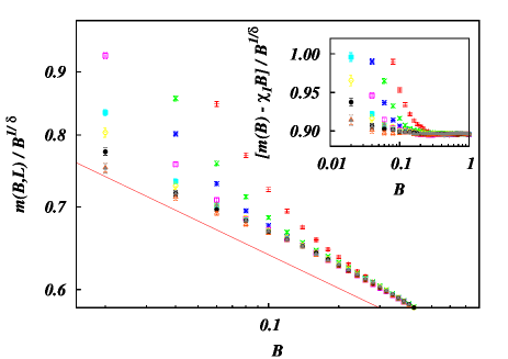
Figure 2: Magnetization divided by $B^{1/\delta}$ as a function of $B$; the $B^{1/1.45}$ line is to guide the eye. From top to bottom, $L=14$, 20, 24, 30, 40, 50, 60, 70, and 80. Inset: $m-\chi_{1}B$ divided by $B^{1/\delta}$ as a function of $B$. (Same $L$ and symbols as in main part of the figure.) In both cases, $\delta$ is set to its droplet model value, $\delta=1.282$.

For that value of $\delta$ there is not much indication that a flat region is developping when $L$ increases, while at $L=50$ a direct fit to a power gives $\delta=1.45$ (cf. line displayed in the figure to guide the eye), as found in previous work Kawashima and Suzuki (1992); Barahona (1994); Rieger et al. (1996). The problem with this simple analysis is that $m$ has both analytic and non-analytic contributions; to lowest order we have

$$m=\chi_{1}B+\chi_{S}B^{1/\delta}+\ldots$$ (7)

Although $\chi_{1}B$ is sub-dominant, it is far from negligible in practice; for instance for it to contribute to less than $10\%$ of $m$, one would need $B<(0.1\chi_{S}/\chi_{1})^{1/0.282}$. This could easily mean $B<10^{-3}$ for which there would be huge finite size effects since $L$ would then be much smaller than the magnetic length $\xi_{B}$. We thus must take into account the term $\chi_{1}B$; we have done this, adjusting $\chi_{1}$ so that $(m-\chi_{1}B)/B^{1/\delta}$ has an envelope as flat as possible. The result is displayed in the inset of Fig. 2, showing that the droplet scaling fits very well the data as long as the $\chi_{1}B$ term is included. In fact, direct fits to the form of Eq. 7 give $\delta$ in the range 1.28 to 1.32 depending on the sets of $L$’s included in the fits.

The clusters that flip are like zero-field droplets —

The fundamental hypothesis in the droplet argument relating $\delta$ or $y_{B}$ to $\theta$ is the fact that in an infinitesimal field one flips droplets defined in zero field, droplets which are compact and have random (except for the sign) magnetizations. We therefore now focus on the properties of the actual clusters that are flipped at low fields.

At zero field, the droplet of lowest energy almost always is a single spin (this follows from the large number of such droplets, in spite of their typically higher energy). Thus as the field is turned on, the ground state changes first mainly via single spin flips, and when large clusters do flip (they finally do so but at larger fields), they necessarily have many “holes” and thus do not correspond exactly to zero-field droplets. This is not a problem for the droplet argument as long as these clusters are compact and have random magnetizations.

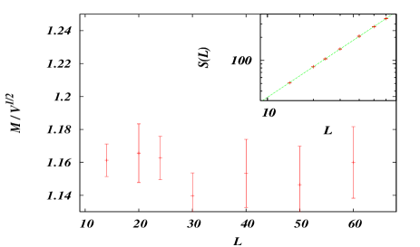
Figure 3: The cluster magnetization divided by the square root of cluster volume — for the largest cluster flipped in each sample — is insensitive to $L$. Inset: The clusters’s mean surface scales as $L^{d_{S}}$ with $d_{S}\approx 1.32$.

To test this, we consider for each realization of the $J_{ij}$ disorder the largest cluster that flips during the whole passage from $B=0$ to $B=\infty$. According to the droplet picture, this cluster should contain a number of spins $V$ that scales as $L^{2}$ (compactness) and have a total magnetization $M$ that scales as $\sqrt{V}$ (randomness). This is confirmed by our data where we find $M/V\sim 2/L$; in Fig. 3 we plot the disorder mean of $M/\sqrt{V}$ for increasing $L$; manifestly, this mean is remarkably insensitive to $L$. Similar conclusions apply to $V/L^{2}$. For completeness, we show in the inset of the figure that the surface of these clusters, defined as the number of lattice bonds connecting them to their complement, grows as $L^{d_{S}}$ with $d_{S}\approx 1.32$; this is to be compared to the value $d_{S}=1.27$ for zero-field droplets Hartmann and Young (2002), in spite of the fact that our clusters have holes. All in all, we find that the clusters considered have statistical properties that are completely compatible with those assumed in the droplet scaling argument, thereby directly validating the associated hypotheses.

The magnetic exponent $y_{B}$ and finite size scaling of the magnetization —

One can also measure the exponent $y_{B}$ directly via the magnetic length which scales as $\xi_{B}\sim B^{-1/y_{B}}$. For each sample, define $B_{J}^{*}$ as that field where the ground state changes by the largest cluster of spins as described in the previous paragraph. Since these clusters involve a number of spins growing as $L^{2}$, we can identify $\xi_{B}(B_{J}^{*})$ with $L$. Let $B^{*}$ be the disorder average of $B_{J}^{*}$; then $B^{*}\sim L^{-y_{B}}$ from which we can estimate $y_{B}$. We find that a pure power with $y_{B}$ set to its value in the droplet picture describes the data quite well; in the inset of Fig. 4

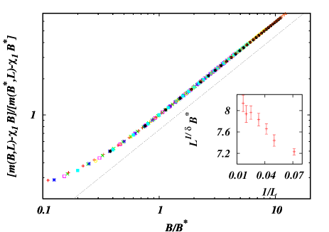
Figure 4: Inset: Field $B^{*}$ times $L^{1/\delta}$ as a function of $1/L$ shows a limit at large $L$ as expected in the droplet model ($\delta=1.282$). Main figure: Data collapse plot exhibiting finite size scaling of the singular part of the magnetization ($L=10$, 14, 20, 24, 30, 40, 50, and 60).

we display the product $L^{1.282}B^{*}$ as a function of $1/L$ and see that the behavior is compatible with a large $L$ limit with $O(1/L)$ finite size effects. Direct fits to the form $B^{*}(L)=uL^{-y_{B}}(1+v/L)$ give $y_{B}$s in the range $1.28$ to $1.30$ depending on the points included in the fit.

Given the magnetic length, one can perform finite size scaling (FSS) on the magnetization data $m(B,L)$. Since FSS applies to the singular part of an observable, we should have a data collapse according to

$$\frac{m(B,L)-\chi_{1}B}{m(B^{*},L)-\chi_{1}B^{*}}=W(B/B^{*})$$ (8)

$W$ being a universal function, $W(0)=O(1)$ and $W(x)\sim x^{1/\delta}$ at large $x$. Using the value of $\chi_{1}$ previously determined, we display in Fig. 4 the associated data. The collapse is excellent and we have checked that this also holds when the $J_{ij}$ are drawn from an exponential distribution. Added to the figure is the function $x^{1/\delta}$ to guide the eye ($\delta=1.282$ as predicted by the droplet model).

Conclusions —

We have investigated the $2d$ Ising spin glass with Gaussian and exponential couplings at zero temperature as a function of the magnetic field. The magnetization exponent $\delta$ can be measured; previous studies did not find good agreement with the droplet model prediction $\delta=1.282$ because the analytic contributions to the magnetization curve were mishandled, while in this work we found instead $1.28\leq\delta\leq 1.32$. We also performed a direct measurement of the magnetic length, obtaining for the associated exponent $1.28\leq y_{B}\leq 1.30$, again in excellent agreement with the droplet prediction. With this length we showed that finite size scaling is realized without going to infinitesimal fields or huge lattices. Finally, we validated the hypotheses underlying the arguments of the droplet model inherent to the in-field case; we find in particular that in the low-field limit the spin clusters that are relevant are compact and have random magnetizations. In summary, by combining improved computational techniques and greater care in the analysis, we have lifted the discrepancy on the magnetic exponents that has existed for over a decade between numerics and droplet scaling.

We thank T. Jorg for helpful comments. The computations were performed on the cliot cluster of the Regional Computing Center and on the scale cluster of E. Speckenmeyer’s group, both in Cologne. FL has been supported by the German Science Foundation in the projects Ju 204/9 and Li 1675/1 and by the Marie Curie RTN ADONET 504438 funded by the EU. This work was supported also by the EEC’s HPP under contract HPRN-CT-2002-00307 (DYGLAGEMEM).

References

- Mézard et al. (1987) M. Mézard, G. Parisi, and M. A. Virasoro, Spin-Glass Theory and Beyond, vol. 9 of Lecture Notes in Physics (World Scientific, Singapore, 1987).
- Young (1998) A. Young, ed., Spin Glasses and Random Fields (World Scientific, Singapore, 1998).
- Katzgraber et al. (2004) H. G. Katzgraber, L. Lee, and A. Young, Phys. Rev. B 70, 014417 (2004).
- Hartmann and Houdayer (2004) A. Hartmann and J. Houdayer, Phys. Rev. B 70, 014418 (2004), cond-mat/0402036.
- Bray and Moore (1986) A. J. Bray and M. A. Moore, in Heidelberg Colloquium on Glassy Dynamics, edited by J. L. van Hemmen and I. Morgenstern (Springer, Berlin, 1986), vol. 275 of Lecture Notes in Physics, pp. 121–153.
- Fisher and Huse (1986) D. S. Fisher and D. A. Huse, Phys. Rev. Lett. 56, 1601 (1986).
- Kinzel and Binder (1983) W. Kinzel and K. Binder, Phys. Rev. Lett. 50, 1509 (1983).
- Kawashima and Suzuki (1992) N. Kawashima and M. Suzuki, J. Phys. A 25, 1055 (1992).
- Barahona (1994) F. Barahona, Phys. Rev. B 49, 12864 (1994).
- Rieger et al. (1996) H. Rieger, L. Santen, U. Blasum, M. Diehl, M. Jünger, and G. Rinaldi, J. Phys. A 29, 3939 (1996).
- Carter et al. (2003) A. Carter, A. Bray, and M. Moore, J. Phys. A 36, 5699 (2003).
- Cardy (1996) J. Cardy, Scaling and renormalization in statistical physics (Cambridge University Press, Cambridge, 1996).
- Barahona (1982) F. Barahona, J. Phys. A 15, 3241 (1982).
- Barahona et al. (1988) F. Barahona, M. Grötschel, M. Jünger, and G. Reinelt, Oper. Res. 36, 493 (1988).
- Liers et al. (2004) F. Liers, M. Jünger, G. Reinelt, and G. Rinaldi, in New Optimization Algorithms in Physics, edited by A. Hartmann and H. Rieger (Wiley-VCH, Berlin, 2004).
- Hartmann and Young (2002) A. Hartmann and A. Young, Phys. Rev. B 66, 094419 (2002), cond-mat/0205659.