On the support genus of a contact structure

Abstract.

The algorithm given by Akbulut and Ozbagci constructs an explicit open book decomposition on a contact three-manifold described by a contact surgery on a link in the three-sphere. In this article, we will improve this algorithm by using Giroux’s contact cell decomposition process. In particular, our algorithm gives a better upper bound for the recently defined “minimal supporting genus invariant” of contact structures.

1. Introduction

Let $(M,\xi)$ be a closed oriented contact 3-manifold, and let $(\Sigma,h)$ be an open book (decomposition) of $M$ which is compatible with the contact structure $\xi$ (sometimes we also say that $(\Sigma,h)$ supports $\xi$). Based on the correspondence theorem (see Theorem 2.3) between contact structures and their supporting open books, the topological invariant $sg(\xi)$ was defined in [EO]. More precisely, we have

$$sg(\xi)=\min\{\,\,g(\Sigma)\,\,|\,\,(\Sigma,h)\text{ an open book decomposition supporting }\xi\}$$

called supporting genus of $\xi$. There are some partial results for this invariant. For instance, we have:

Theorem 1.1 ([Et1]).

If $(M,\xi)$ is overtwisted, then $sg(\xi)=0.$

Unlike the overtwisted case, there is not much known yet for $sg(\xi)$ when $\xi$ is tight. On the other hand, if we, furthermore, require that $\xi$ is Stein fillable, then an algorithm to find an open book supporting $\xi$ was given in [AO]. Although their construction is explicit, the pages of the resulting open books arise as Seifert surfaces of torus knots or links, and so this algorithm is far from even approximating the numbers $sg(\xi)$. In [St], the same algorithm was generalized to the case where $\xi$ need not to be Stein fillable (or even tight), but the pages are still of large genera.

This article is organized as follows: After the preliminaries (Section 2), in Section 3 we will present an explicit construction of a supporting open book (with considerably less genus) for a given contact surgery diagram of any contact structure $\xi$. Of course, because of Theorem 1.1, our algorithm makes more sense for the tight structures than the overtwisted ones. Moreover, it depends on a choice of the contact surgery diagram describing $\xi$. Nevertheless, it gives better and more reasonable upper bound for $sg(\xi)$ (when $\xi$ is tight) as we will see from our examples in Section 4.

Let $L$ be any Legendrian link given in $(\mathbb{R}^{3},\xi_{0}=ker(\alpha_{0}=dz+xdy))\subset(S^{3},\xi_{st})$. $L$ can be represented by a special diagram $\mathcal{D}$ called a square bridge diagram of $L$ (see [Ly]). We will consider $\mathcal{D}$ as an abstract diagram such that

1. $\mathcal{D}$ consists of horizontal line segments $h_{1},...,h_{p}$, and vertical line segments $v_{1},...,v_{q}$ for some integers $p\geq 2$, $q\geq 2$,

2. there is no collinearity in $\{h_{1},\dots,h_{p}\}$, and in $\{v_{1},\dots,v_{q}\}$.

3. each $h_{i}$ (resp., each $v_{j}$) intersects two vertical (resp., horizontal) line segments of $\mathcal{D}$ at its two endpoints (called corners of $\mathcal{D}$), and

4. any interior intersection (called junction of $\mathcal{D}$) is understood to be a virtual crossing of $\mathcal{D}$ where the horizontal line segment is passing over the vertical one.

We depict Legendrian right trefoil and the corresponding $\mathcal{D}$ in Figure 1.

Figure 1. The square bridge diagram $\mathcal{D}$ for the Legendrian right trefoil

Clearly, for any front projection of a Legendrian link, we can associate a square bridge diagram $\mathcal{D}$. Using such a diagram $\mathcal{D}$, the following two facts were first proved in [AO], and later made more explicit in [Pl]. Below versions are from the latter:

Lemma 1.2.

Given a Legendrian link $L$ in $(\mathbb{R}^{3},\xi_{0})$, there exists a torus link $T_{p,q}$ (with $p$ and $q$ as above) transverse to $\xi_{0}$ such that its Seifert surface $F_{p,q}$ contains $L$, $d\alpha_{0}$ is an area form on $F_{p,q}$, and $L$ does not separate $F_{p,q}$.

Proposition 1.3.

Given $L$ and $F_{p,q}$ as above, there exist an open book decomposition of $S^{3}$ with page $F_{p,q}$ such that:

1. the induced contact structure $\xi$ is isotopic to $\xi_{0}$;

2. the link $L$ is contained in one of the page $F_{p,q}$, and does not separate it;

3. $L$ is Legendrian with respect to $\xi$;

4. there exist an isotopy which fixes $L$ and takes $\xi$ to $\xi_{0}$, so the Legendrian type of the link is the same with respect to $\xi$ and $\xi_{0}$;

5. the framing of $L$ given by the page $F_{p,q}$ of the open book is the same as the contact framing.

Being a Seifert surface of a torus link, $F_{p,q}$ is of large genera. In Section 3, we will construct another open book $\mathcal{OB}$ supporting $(S^{3},\xi_{st})$ such that its page $F$ arises as a subsurface of $F_{p,q}$ (with considerably less genera), and given Legendrian link $L$ sits on $F$ as how it sits on the page $F_{p,q}$ of the construction used in [AO] and [Pl]. The page $F$ of the open book $\mathcal{OB}$ will arise as the ribbon of the 1-skeleton of an appropriate contact cell decomposition for $(S^{3},\xi_{st})$. As in [Pl], our construction will keep the given link $L$ Legendrian with respect to the standard contact structure $\xi_{st}$. Our main theorem is:

Theorem 1.4.

Given $L$ and $F_{p,q}$ as above, there exists a contact cell decomposition $\Delta$ of $(S^{3},\xi_{st})$ such that

1. $L$ is contained in the Legendrian 1-skeleton $G$ of $\Delta$,

2. The ribbon $F$ of the 1-skeleton $G$ is a subsurface of $F_{p,q}$ ($p$ and $q$ as above),

3. The framing of $L$ coming from $F$ is equal to its contact framing $tb(L)$, and

4. If $p>3$ and $q>3$, then the genus $g(F)$ of $F$ is strictly less than the genus $g(F_{p,q})$ of $F_{p,q}$.

As an immediate consequence (see Corollary 3.1), we get an explicit description of an open book supporting $(S^{3},\xi)$ whose page $F$ contains $L$ with the correct framing. Therefore, if $(M^{\pm},\xi^{\pm})$ is given by contact ($\pm 1$)-surgery on $L$ (such a surgery diagram exists for any closed contact 3-manifold by Theorem 2.1), we get an open book supporting $\xi^{\pm}$ with page $F$ by Theorem 2.5. Hence, $g(F)$ improves the upper bound for $sg(\xi)$ as $g(F)<g(F_{p,q})$ (for $p>3,\;q>3$). It will be clear from our examples in Section 4 that this is indeed a good improvement.

Acknowledgments. The author would like to thank Selman Akbulut, Selahi Durusoy, Cagri Karakurt, and Burak Ozbagci for their helpful conversations and comments on the draft of this paper.

2. Preliminaries

2.1. Contact structures and Open book decompositions

A $1$-form $\alpha\in\Omega^{1}(M)$ on a $3$-dimensional oriented manifold $M$ is called a contact form if it satisfies $\alpha\wedge d\alpha\neq 0$. An oriented contact structure on $M$ is then a hyperplane field $\xi$ which can be globally written as the kernel of a contact $1$-form $\alpha$. We will always assume that $\xi$ is a positive contact structure, that is, $\alpha\wedge d\alpha>0$. Note that this is equivalent to asking that $d\alpha$ be positive definite on the plane field $\xi$, ie., $d\alpha|_{\xi}>0$. Two contact structures $\xi_{0},\xi_{1}$ on a $3$-manifold are said to be isotopic if there exists a 1-parameter family $\xi_{t}$ ($0\leq t\leq 1$) of contact structures joining them. We say that two contact $3$-manifolds $(M_{1},\xi_{1})$ and $(M_{2},\xi_{2})$ are contactomorphic if there exists a diffeomorphism $f:M_{1}\longrightarrow M_{2}$ such that $f_{\ast}(\xi_{1})=\xi_{2}$. Note that isotopic contact structures give contactomorphic contact manifolds by Gray’s Theorem. Any contact $3$-manifold is locally contactomorphic to $(\mathbb{R}^{3},\xi_{0})$ where standard contact structure $\xi_{0}$ on $\mathbb{R}^{3}$ with coordinates $(x,y,z)$ is given as the kernel of $\alpha_{0}=dz+xdy$. The standard contact structure $\xi_{st}$ on the $3$-sphere $S^{3}=\{(r_{1},r_{2},\theta_{1},\theta_{2}):r_{1}^{2}+r_{2}^{2}=1\}\subset\mathbb{C}^{2}$ is given as the kernel of $\alpha_{st}=r_{1}^{2}d\theta_{1}+r_{2}^{2}d\theta_{2}$. One basic fact is that $(\mathbb{R}^{3},\xi_{0})$ is contactomorphic to $(S^{3}\setminus\{pt\},\xi_{st})$. For more details on contact geometry, we refer the reader to [Ge], [Et3].

An open book decomposition of a closed $3$-manifold $M$ is a pair $(L,f)$ where $L$ is an oriented link in $M$, called the binding, and $f:M\setminus L\to S^{1}$ is a fibration such that $f^{-1}(t)$ is the interior of a compact oriented surface $\Sigma_{t}\subset M$ and $\partial\Sigma_{t}=L$ for all $t\in S^{1}$. The surface $\Sigma=\Sigma_{t}$, for any $t$, is called the page of the open book. The monodromy of an open book $(L,f)$ is given by the return map of a flow transverse to the pages (all diffeomorphic to $\Sigma$) and meridional near the binding, which is an element $h\in Aut(\Sigma,\partial\Sigma)$, the group of (isotopy classes of) diffeomorphisms of $\Sigma$ which restrict to the identity on $\partial\Sigma$ . The group $Aut(\Sigma,\partial\Sigma)$ is also said to be the mapping class group of $\Sigma$, and denoted by $\Gamma(\Sigma)$.

An open book can also be described as follows. First consider the mapping torus

$$\Sigma(h)=[0,1]\times\Sigma/(1,x)\sim(0,h(x))$$

where $\Sigma$ is a compact oriented surface with $n=|\partial\Sigma|$ boundary components and $h$ is an element of $Aut(\Sigma,\partial\Sigma)$ as above. Since $h$ is the identity map on $\partial\Sigma$, the boundary $\partial\Sigma(h)$ of the mapping torus $\Sigma(h)$ can be canonically identified with $n$ copies of $T^{2}=S^{1}\times S^{1}$, where the first $S^{1}$ factor is identified with $[0,1]/(0\sim 1)$ and the second one comes from a component of $\partial\Sigma$. Now we glue in $n$ copies of $D^{2}\times S^{1}$ to cap off $\Sigma(h)$ so that $\partial D^{2}$ is identified with $S^{1}=[0,1]/(0\sim 1)$ and the $S^{1}$ factor in $D^{2}\times S^{1}$ is identified with a boundary component of $\partial\Sigma$. Thus we get a closed $3$-manifold

$$M=M_{(\Sigma,h)}:=\Sigma(h)\cup_{n}D^{2}\times S^{1}$$

equipped with an open book decomposition $(\Sigma,h)$ whose binding is the union of the core circles in the $D^{2}\times S^{1}$’s that we glue to $\Sigma(h)$ to obtain $M$. To summarize, an element $h\in Aut(\Sigma,\partial\Sigma)$ determines a $3$-manifold $M=M_{(\Sigma,h)}$ together with an “abstract” open book decomposition $(\Sigma,h)$ on it. For furher details on these subjects, see [Gd], and [Et2].

2.2. Legendrian Knots and Contact Surgery

A Legendrian knot $K$ in a contact $3$-manifold $(M,\xi)$ is a knot that is everywhere tangent to $\xi$. Any Legendrian knot comes with a canonical contact framing (or Thurston-Bennequin framing), which is defined by a vector field along $K$ that is transverse to $\xi$. If $K$ is null-homologous, then this framing can be given by an integer $tb(K)$, called Thurston-Bennequin number. For any Legendrian knot $K$ in $(\mathbb{R}^{3},\xi_{0})$, the number $tb(K)$ can be computed as

$$tb(K)=bb(K)-\#\mbox{left cusps of K}$$

where $bb(K)$ is the blackboard framing of $K$.

We call $(M,\xi)$ (or just $\xi$) overtwisted if it contains an embedded disc $D\approx D^{2}\subset M$ with boundary $\partial D\approx S^{1}$ a Legendrian knot whose contact framing equals the framing it receives from the disc $D$. If no such disc exists, the contact structure $\xi$ is called tight.

For any $p,q\in\mathbb{Z}$, a contact $(r)$-surgery ($r=p/q$) along a Legendrian knot $K$ in a contact manifold $(M,\xi)$ was first described in [DG1]. It is defined to be a special kind of a topological surgery, where surgery coefficient $r\in{\mathbb{Q}}\cup{\infty}$ measured relative to the contact framing of $K$. For $r\neq 0$, a contact structure on the surgeried manifold

$$(M-\nu K)\cup(S^{1}\times D^{2}),$$

($\nu K$ denotes a tubular neighborhood of $K$) is defined by requiring this contact structure to coincide with $\xi$ on $Y-\nu K$ and its extension over $S^{1}\times D^{2}$ to be tight on (glued in) solid torus $S^{1}\times D^{2}$. Such an extension uniquely exists (up to isotopy) for $r=1/k$ with $k\in\mathbb{Z}$ (see [Ho]). In particular, a contact $(\pm 1)$-surgery along a Legendrian knot $K$ on a contact manifold $(M,\xi)$ determines a unique (up to contactomorphism) surgered contact manifold which will be denoted by $(M,\xi)_{(K,\pm 1)}$.

The most general result along these lines is:

Theorem 2.1 ([DG1]).

Every (closed, orientable) contact $3$-manifold $(M,\xi)$ can be obtained via contact $(\pm 1)$-surgery on a Legendrian link in $(S^{3},\xi_{st})$.

Any closed contact $3$-manifold $(M,\xi)$ can be described by a contact surgery diagram. Such a diagram consists of a front projection (onto the $yz$-plane) of a Legendrian link drawn in $(\mathbb{R}^{3},\xi_{0})\subset(S^{3},\xi_{st})$ with contact surgery coefficient on each link component. Theorem 2.1 implies that there is a contact surgery diagram for $(M,\xi)$ such that the contact surgery coefficient of any Legendrian knot in the diagram is $\pm 1$. For more details see [Gm] and [OS].

2.3. Compatibility and Stabilization

A contact structure $\xi$ on a $3$-manifold $M$ is said to be supported by an open book $(L,f)$ if $\xi$ is isotopic to a contact structure given by a $1$-form $\alpha$ such that

1. $d\alpha$ is a positive area form on each page $\Sigma\approx f^{-1}($pt$)$ of the open book and

2. $\alpha>0$ on $L$ (Recall that $L$ and the pages are oriented.)

When this holds, we also say that the open book $(L,f)$ is compatible with the contact structure $\xi$ on $M$. Geometrically, compatibility means that $\xi$ can be isotoped to be arbitrarily close (as oriented plane fields), on compact subsets of the pages, to the tangent planes to the pages of the open book in such a way that after some point in the isotopy the contact planes are transverse to $L$ and transverse to the pages of the open book in a fixed neighborhood of $L$.

Definition 2.2.

A positive (resp., negative) stabilization $S^{+}_{K}(\Sigma,h)$ (resp., $S^{-}_{K}(\Sigma,h)$) of an abstract open book $(\Sigma,h)$ is the open book

1. with page $\Sigma^{\prime}=\Sigma\cup\text{ 1-handle}$ and

2. monodromy $h^{\prime}=h\circ D_{K}$ (resp., $h^{\prime}=h\circ D_{K}^{-1}$) where $D_{K}$ is a right-handed Dehn twist along a curve $K$ in $\Sigma^{\prime}$ that intersects the co-core of the 1-handle exactly once.

Based on the result of Thurston and Winkelnkemper [TW], Giroux proved the following theorem which strengthened the link between open books and contact structures.

Theorem 2.3 ([Gi]).

Let $M$ be a closed oriented $3$-manifold. Then there is a one-to-one correspondence between oriented contact structures on $M$ up to isotopy and open book decompositions of $M$ up to positive stabilizations: Two contact structures supported by the same open book are isotopic, and two open books supporting the same contact structure have a common positive stabilization.

For a given fixed open book $(\Sigma,h)$ of a $3$-manifold $M$, there exists a unique compatible contact structure up to isotopy on $M=M_{(\Sigma,h)}$ by Theorem 2.3. We will denote this contact structure by $\xi_{(\Sigma,h)}$. Therefore, an open book $(\Sigma,h)$ determines a unique contact manifold $(M_{(\Sigma,h)},\xi_{(\Sigma,h)})$ up to contactomorphism.

Taking a positive stabilization of an open book $(\Sigma,h)$ is actually taking a special Murasugi sum of $(\Sigma,h)$ with $(H^{+},D_{c})$ where $H^{+}$ is the positive Hopf band, and $c$ is the core circle in $H^{+}$. Taking a Murasugi sum of two open books corresponds to taking the connect sum of $3$-manifolds associated to the open books. For the precise statements of these facts, and a proof of the following theorem, we refer the reader to [Gd], [Et2].

Theorem 2.4.

$(M_{S^{+}_{K}(\Sigma,h)},\xi_{S^{+}_{K}(\Sigma,h)})\cong(M_{(\Sigma,h)},\xi_{(\Sigma,h)})\#(S^{3},\xi_{st})\cong(M_{(\Sigma,h)},\xi_{(S,h)}).$

2.4. Monodromy and Surgery Diagrams

Given a contact surgery diagram for a closed contact $3$-manifold $(M,\xi)$, we want to construct an open book compatible with $\xi$. One implication of Theorem 2.1 is that one can obtain such a compatible open book by starting with a compatible open book of $(S^{3},\xi_{st})$, and then interpreting the effects of surgeries (yielding $(M,\xi)\,$) in terms of open books. However, we first have to realize each surgery curve (in the given surgery diagram of $(M,\xi)\,$) as a Legendrian curve sitting on a page of some open book supporting $(S^{3},\xi_{st})$. We refer the reader to Section 5 in [Et2] for a proof of the following theorem.

Theorem 2.5.

Let $(\Sigma,h)$ be an open book supporting the contact manifold $(M,\xi).$ If $K$ is a Legendrian knot on the page $\Sigma$ of the open book, then

$$(M,\xi)_{(K,\;\pm 1)}=(M_{(\Sigma,\;h\circ D_{K}^{\mp})},\xi_{(\Sigma,\;h\circ D_{K}^{\mp})}).$$

2.5. Contact Cell Decompositions and Convex Surfaces

The exploration of contact cell decompositions in the study of open books was originally initiated by Gabai [Ga], and then developed by Giroux [Gi]. We want to give several definitions and facts carefully.

Let $(M,\xi)$ be any contact 3-manifold, and $K\subset M$ be a Legendrian knot. The twisting number $tw(K,Fr)$ of $K$ with respect to a given framing $Fr$ is defined to be the number of counterclockwise $2\pi$ twists of $\xi$ along $K$, relative to $Fr$. In particular, if $K$ sits on a surface $\Sigma\subset M$, and $Fr_{\Sigma}$ is the surface framing of $K$ given by $\Sigma$, then we write $tw(K,\Sigma)$ for $tw(K,Fr_{\Sigma})$. If $K=\partial\Sigma$, then we have $tw(K,\Sigma)=tb(K)$ (by the definition of $\,tb$).

Definition 2.6.

A contact cell decomposition of a contact $3-$manifold $(M,\xi)$ is a finite CW-decomposition of $M$ such that

1. the 1-skeleton is a Legendrian graph,

2. each 2-cell $D$ satisfies $tw(\partial D,D)=-1,$ and

3. $\xi$ is tight when restricted to each 3-cell.

Definition 2.7.

Given any Legendrian graph $G$ in $(M,\xi)$, the ribbon of $G$ is a compact surface $R=R_{G}$ satisfying

1. $R$ retracts onto $G,$

2. $T_{p}R=\xi_{p}$ for all $p\in G,$

3. $T_{p}R\not=\xi_{p}$ for all $p\in R\setminus G.$

For a proof of the following lemma we refer the reader to [Gd] and [Et2].

Lemma 2.8.

Given a closed contact $3-$manifold $(M,\xi)$, the ribbon of the 1-skeleton of any contact cell decomposition is a page of an open book supporting $\xi$.

The following lemma will be used in the next section.

Lemma 2.9.

Let $\Delta$ be a contact cell decomposition of a closed contact 3-manifold $(M,\xi)$ with the $1-$skeleton $G$. Let $U$ be a 3-cell in $\Delta$. Consider two Legendrian arcs $I\subset\partial U$ and $J\subset U$ such that

1. $I\subset G$,

2. $J\cap\partial U=\partial J=\partial I$,

3. $C=I\cup_{\partial}J$ is a Legendrian unknot with $tb(C)=-1$.

Set $G^{\prime}=G\cup J$. Then there exists another contact cell decomposition $\Delta^{\prime}$ of $(M,\xi)$ such that $G^{\prime}$ is the 1-skeleton of $\Delta^{\prime}$

Proof.

The interior of the $3-$cell $U$ is contactomorphic to $(\mathbb{R}^{3},\xi_{0})$. Therefore, there exists an embedded disk $D$ in $U$ such that $\partial D=C$ and $int(D)\subset int(U)$ as depicted in Figure 2(a). We have $tw(\partial D,D)=-1$ since $tb(C)=-1$. As we are working in $(\mathbb{R}^{3},\xi_{0})$, there exist two $C^{\infty}$-small perturbations of $D$ fixing $\partial D=C$ such that perturbed disks intersect each other only along their common boundary $C$. In other words, we can find two isotopies $H_{1},H_{2}:[0,1]\times D\longrightarrow U$ such that for each $i=1,2$ we have

1. $H_{i}(t,.)$ fixes $\partial D=C$ pointwise for all $t\in[0,1]$,

2. $H_{i}(0,D)=Id_{D}$ where $Id_{D}$ is the identity map on $D$,

3. $H_{i}(1,D)=D_{i}$ where each $D_{i}$ is an embedded disk in $U$ with $int(D_{i})\subset int(U)$,

4. $D\cap D_{1}\cap D_{2}=C$ (see Figure 2(b)).

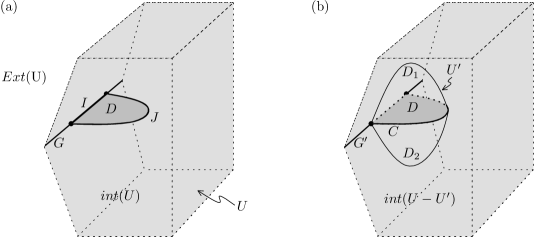
Figure 2. Constructing a new contact cell decomposition

Note that $tw(\partial D_{i},D_{i})=tw(C,D_{i})=-1$ for $i=1,2$. This holds because each $D_{i}$ is a small perturbation of $D$, so the number of counterclockwise twists of $\xi$ (along $K$) relative to $Fr_{D_{i}}$ is equal to the one relative to $Fr_{D}$.

Next, we introduce $G^{\prime}=G\cup J$ as the 1-skeleton of the new contact cell decomposition $\Delta^{\prime}$. In $M-int(U)$, we define the 2- and 3- skeletons of $\Delta^{\prime}$ to be those of $\Delta$ . However, we change the cell structure of $int(U)$ as follows: We add 2-cells $D_{1},D_{2}$ to the 2-skeleton of $\Delta^{\prime}$ (note that they both satisfy the twisting condition in Definition 2.6). Consider the 2-sphere $S=D_{1}\cup D_{2}$ where the union is taken along the common boundary $C$. Let $U^{\prime}$ be the 3-ball with $\partial U^{\prime}=S$. Note that $\xi|_{U^{\prime}}$ is tight as $U^{\prime}\subset U$ and $\xi|U$ is tight. We add $U^{\prime}$ and $U-U^{\prime}$ to the 3-skeleton of $\Delta^{\prime}$ (note that $U-U^{\prime}$ can be considered as a 3-cell because observe that $int(U-U^{\prime})$ is homeomorphic to the interior of a 3-ball as in Figure 2(b)). Hence, we established another contact cell decomposition of $(M,\xi)$ whose 1-skeleton is $G^{\prime}=G\cup J$. (Equivalently, by Theorem 2.4, we are taking the connect sum of $(M,\xi)$ with $(S^{3},\xi_{st})$ along $U^{\prime}$.) ∎

3. The Algorithm

3.1. Proof of Theorem 1.4

Proof.

By translating $L$ in $(\mathbb{R}^{3},\xi_{0})$ if necessary (without changing its contact type), we can assume that the front projection of $L$ onto the $yz$-plane lying in the second quadrant $\{\;(y,z)\;|\;y<0,\;z>0\}$. After an appropriate Legendrian isotopy, we can assume that $L$ consists of the line segments contained in the lines

$k_{i}=\{x=1,z=-y+a_{i}\}$, $i=1,\dots,p$,

$l_{j}=\{x=-1,z=y+b_{j}\}$, $j=1,\dots,q$

for some $a_{1}<a_{2}<\dots<a_{p}$, $0<b_{1}<b_{2}<\dots<b_{q}$, and also the line segments (parallel to the $x$-axis) joining certain $k_{i}$’s to certain $l_{j}$’s. In this representation, $L$ seems to have corners. However, any corner of $L$ can be made smooth by a Legendrian isotopy changing only a very small neighborhood of that corner.

Let $\pi:\mathbb{R}^{3}\longrightarrow\mathbb{R}^{2}$ be the projection onto the $yz$-plane. Then we obtain the square bridge diagram $D=\pi(L)$ of $L$ such that $D$ consists of the line segments

$$h_{i}\subset\pi(k_{i}) = \{x=0,z=-y+a_{i}\},\quad i=1,\dots,p,$$

$$v_{j}\subset\pi(l_{j}) = \{x=0,z=y+b_{j}\},\quad j=1,\dots,q.$$

Notice that $D$ bounds a polygonal region $P$ in the second quadrant of the $yz$-plane, and divides it into finitely many polygonal subregions $P_{1},\dots,P_{m}$ ( see Figure 3-(a) ).

Throughout the proof, we will assume that the link $L$ is not split (that is, the region $P$ has only one connected component). Such a restriction on $L$ will not affect the generality of our construction (see Remark 3.2).

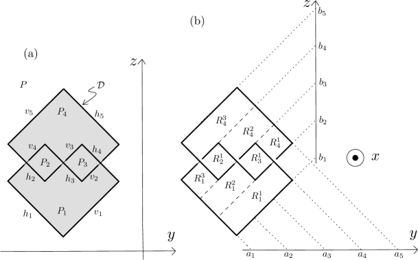
Figure 3. The region $P$ for right trefoil knot and its division into rectangles

Now we decompose $P$ into finite number of ordered rectangular subregions as follows: The collection $\{\pi(l_{j})\;|\;j=1,\dots,q\}$ cuts each $P_{k}$ into finitely many rectangular regions $R_{k}^{1},\dots,R_{k}^{m_{k}}$. Consider the set $\mathfrak{P}$ of all such rectangles in $P$. That is, we define

$\mathfrak{P}\doteq\{\;R_{k}^{l}\;|\;k=1,\dots,m,\quad l=1,\dots,m_{k}\}$.

Clearly $\mathfrak{P}$ decomposes $P$ into rectangular regions ( see Figure 3-(b) ). The boundary of an arbitrary element $R_{k}^{l}$ in $\mathfrak{P}$ consists of four edges: Two of them are the subsets of the lines $\pi(l_{j(k,l)})$, $\pi(l_{j(k,l)+1})$, and the other two are the subsets of the line segments $h_{i_{1}(k,l)}$, $h_{i_{2}(k,l)}$ where $1\leq i_{1}(k,l)<i_{2}(k,l)\leq p$ and $1\leq j(k,l)<j(k,l)+1\leq q$ (see Figure 4).

Figure 4. Arbitrary element $R_{k}^{l}$ in $\mathfrak{P}$

Since the region $P$ has one connected component, the following holds for the set $\mathfrak{P}$:

($\star$) Any element of $\mathfrak{P}$ has at least one common vertex with some other element of $\mathfrak{P}$.

By ($\star$), we can rename the elements of $\mathfrak{P}$ by putting some order on them so that any element of $\mathfrak{P}$ has at least one vertex in common with the union of all rectangles coming before itself with respect to the chosen order. More precisely, we can write

$$\mathfrak{P}=\{\;R_{k}\;|\;k=1,\dots,N\}$$

($N$ is the total number of rectangles in $\mathfrak{P}$) such that each $R_{k}$ has at least one vertex in common with the union $R_{1}\cup\dots\cup R_{k-1}$.

Equivalently, we can construct the polygonal region $P$ by introducing the building rectangles ($R_{k}$’s) one by one in the order given by the index set $\{1,2,\dots,N\}$. In particular, this eliminates one of the indexes, i.e., we can use $R_{k}$’s instead of $R_{k}^{l}$’s. In Figure 5, how we build $P$ is depicted for the right trefoil knot (compare it with the previous picture given for $P$ in Figure 3-(b)).

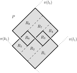
Figure 5. The region $P$ for right trefoil knot

Using the representation $P=R_{1}\cup R_{2}\cup\dots\cup R_{N}$, we will construct the contact cell decomposition (CCD) $\Delta$. Consider the following infinite strips which are parallel to the $x$-axis (they can be considered as the unions of “small” contact planes along $k_{i}$’s and $l_{j}$’s):

$$S^{+}_{i} = \{1-\epsilon\leq x\leq 1+\epsilon,\;z=y+a_{i}\},\;i=1,\dots,p,$$

$$S^{-}_{j} = \{-1-\epsilon\leq x\leq-1+\epsilon,\;z=-y+b_{j}\},\;j=1,\dots,q.$$

Note that $\pi(S^{+}_{i})=\pi(k_{i})$ and $\pi(S^{-}_{j})=\pi(l_{j})$. Let $R_{k}\subset P$ be given. Then we can write

$\partial R_{k}=C_{k}^{1}\cup C_{k}^{2}\cup C_{k}^{3}\cup C_{k}^{4}$ where $C_{k}^{1}\subset\pi(k_{i_{1}})$, $C_{k}^{2}\subset\pi(l_{j})$, $C_{k}^{3}\subset\pi(k_{i_{2}})$, $C_{k}^{4}\subset\pi(l_{j+1})$

for some $1\leq i_{1}<i_{2}\leq p$ and $1\leq j\leq q$. Lift $C_{k}^{1},C_{k}^{2},C_{k}^{3},C_{k}^{4}$ (along the $x$-axis) so that the resulting lifts (which will be denoted by the same letters) are disjoint Legendrian arcs contained in $k_{i_{1}},l_{j},k_{i_{2}},l_{j+1}$ and sitting on the corresponding strips $S^{+}_{i_{1}},S^{-}_{j},S^{+}_{i_{2}},S^{-}_{j+1}$. For $l=1,2,3,4$, consider Legendrian linear arcs $I_{k}^{l}$ (parallel to the $x$-axis) running between the endpoints of $C_{k}^{l}$’s as in Figure 6-(a)&(b). Along each $I_{k}^{l}$ the contact planes make a $90^{\circ}$ left-twist. Let $B_{k}^{l}$ be the narrow band obtained by following the contact planes along $I_{k}^{l}$. Then define $F_{k}$ to be the surface constructed by taking the union of the compact subsets of the above strips (containing corresponding $C_{k}^{l}$’s) with the bands $B_{k}^{l}$’s (see Figure 6-(b)). $C_{k}^{l}$’s and $I_{k}^{l}$’s together build a Legendrian unknot $\gamma_{k}$ in $(\mathbb{R}^{3},\xi_{0})$, i.e., we set

$$\gamma_{k}=C_{k}^{1}\cup I_{k}^{1}\cup C_{k}^{2}\cup I_{k}^{2}\cup C_{k}^{3}\cup I_{k}^{3}\cup C_{k}^{4}\cup I_{k}^{4}.$$

Note that $\pi(\gamma_{k})=\partial R_{k}$, $\gamma_{k}$ sits on the surface $F_{k}$, and $F_{k}$ deformation retracts onto $\gamma_{k}$. Indeed, by taking all strips and bands in the construction small enough, we may assume that contact planes are tangent to the surface $F_{k}$ only along the core circle $\gamma_{k}$. Thus, $F_{k}$ is the ribbon of $\gamma_{k}$. Observe that, topologically, $F_{k}$ is a positive (left-handed) Hopf band.

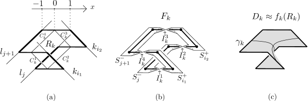
Figure 6. (a) The Legendrian unknot $\gamma_{k}$, (b) The ribbon $F_{k}$, (c) The disk $D_{k}$ (shaded bands in (b) are the bands $B_{k}^{l}$’s)

Let $f_{k}:R_{k}\longrightarrow\mathbb{R}^{3}$ be a function modelled by $(a,b)\mapsto c=a^{2}-b^{2}$ (for an appropriate choice of coordinates). The image $f_{k}(R_{k})$ is, topologically, a disk, and a compact subset of a saddle surface. Deform $f_{k}(R_{k})$ to another “saddle” disk $D_{k}$ such that $\partial D_{k}=\gamma_{k}$ (see Figure 6-(c)). We observe here that $tw(\gamma_{k},D_{k})=-1$ because along $\gamma_{k}$, contact planes rotate $90^{\circ}$ in the counter-clockwise direction exactly four times which makes one full left-twist (enough to count the twists of the ribbon $F_{k}$ since $F_{k}$ rotates with the contact planes along $\gamma_{k}$ !).

We repeat the above process for each rectangle $R_{k}$ in $P$ and get the set

$$\mathfrak{D}=\{\;D_{k}\;|\;D_{k}\approx f_{k}(R_{k}),\;k=1,\dots,N\}$$

consisting of the saddle disks. Note that by the construction of $\mathfrak{D}$, we have the property:

     ($\ast$) If any two elements of $\mathfrak{D}$ intersect each other, then they must intersect along a     contractible subset (a contractible union of linear arcs) of their boundaries.

For instance, if the corresponding two rectangles (for two intersecting disks in $\mathfrak{D}$) have only one common vertex, then those disks intersect each other along the (contractible) line segment parallel to the $x$-axis which is projected (by the map $\pi$) onto that vertex.

For each $k$, let $D_{k}^{\prime}$ be a disk constructed by perturbing $D_{k}$ slightly by an isotopy fixing only the boundary of $D_{k}$. Therefore, we have

($\ast\ast$) $\partial D_{k}=\gamma_{k}=\partial D_{k}^{\prime}\;$, $\quad int(D_{k})\cap int(D_{k}^{\prime})=\emptyset\;$, and $\quad tw(\gamma_{k},D_{k}^{\prime})=-1=tw(\gamma_{k},D_{k})$.

In the following, we will define a sequence $\{\;\Delta_{k}\;|\;k=1,\dots,N\;\}$ of CCD’s for $(S^{3},\xi_{st})$. $\Delta_{k}^{1},\Delta_{k}^{2}$, and $\Delta_{k}^{3}$ will denote the 1-skeleton, 2-skeleton, and 3-skeleton of $\Delta_{k}$, respectively. First, take $\Delta_{1}^{1}=\gamma_{1}$, and $\Delta_{1}^{2}=D_{1}\cup_{\gamma_{1}}D_{1}^{\prime}$. By ($\ast\ast$), $\Delta_{1}$ satisfies the conditions (1) and (2) of Definition 2.6. By the construction, any pair of disks $D_{k},D_{k}^{\prime}$ (together) bounds a Darboux ball (tight 3-cell) $U_{k}$ in the tight manifold $(\mathbb{R}^{3},\xi_{0})$. Therefore, if we take $\Delta_{1}^{3}=U_{1}\cup_{\partial}(S^{3}-U_{1})$, we also achieve the condition (3) in Definition 2.6 ( the boundary union “ $\cup_{\partial}$” is taken along $\partial U_{1}=S^{2}=\partial(S^{3}-U_{1})$ ). Thus, $\Delta_{1}$ is a CCD for $(S^{3},\xi_{st})$.

Inductively, we define $\Delta_{k}$ from $\Delta_{k-1}$ by setting

$$\Delta_{k}^{1} = \Delta_{k-1}^{1}\cup\gamma_{k}=\gamma_{1}\cup\dots\cup\gamma_{k-1}\cup\gamma_{k},$$

$$\Delta_{k}^{2} = \Delta_{k-1}^{2}\cup D_{k}\cup_{\gamma_{k}}D_{k}^{\prime}=D_{1}\cup_{\gamma_{1}}D_{1}^{\prime}\cup\dots\cup D_{k-1}\cup_{\gamma_{k-1}}D_{k-1}^{\prime}\cup D_{k}\cup_{\gamma_{k}}D_{k}^{\prime},$$

$$\Delta_{k}^{3} = U_{1}\cup\dots\cup U_{k-1}\cup U_{k}\cup_{\partial}(S^{3}-U_{1}\cup\dots\cup U_{k-1}\cup U_{k})$$

Actually, at each step of the induction, we are applying Lemma 2.9 to $\Delta_{k-1}$ to get $\Delta_{k}$. We should make several remarks: First, by the construction of $\gamma_{k}$’s, the set

$$(\gamma_{1}\cup\dots\cup\gamma_{k-1})\cap\gamma_{k}$$

is a contractible union of finitely many arcs. Therefore, the union $\Delta_{k-1}^{1}\cup\gamma_{k}$ should be understood to be a set-theoretical union (not a topological gluing!) which means that we are attaching only the (connected) part ($\gamma_{k}\setminus\Delta_{k-1}^{1}$) of $\gamma_{k}$ to construct the new 1-skeleton $\Delta_{k}^{1}$. In terms of the language of Lemma 2.9, we are setting $I=\Delta_{k-1}^{1}\setminus\gamma_{k}$ and $J=\gamma_{k}\setminus\Delta_{k-1}^{1}$. Secondly, we have to show that $\Delta_{k}^{2}=\Delta_{k-1}^{2}\cup D_{k}\cup_{\gamma_{k}}D_{k}^{\prime}$ can be realized as the 2-skeleton of a CCD: Inductively, we can achieve the twisting condition on 2-cells by using ($\ast\ast$). The fact that any two intersecting 2-cells in $\Delta_{k}^{2}$ intersect each other along some subset of the 1-skeleton $\Delta_{k}^{1}$ is guaranteed by the property $(\ast)$ if they have different index numbers, and guaranteed by $(\ast\ast)$ if they are of the same index. Thirdly, we have to guarantee that 3-cells meet correctly: It is clear that $U_{1},\dots,U_{k}$ meet with each other along subsets of the 1-skeleton $\Delta_{k}^{1}(\subset\Delta_{k}^{2})$. Observe that $\partial(U_{1}\cup\dots\cup U_{k})=S^{2}$ for any $k=1,\dots,N$ by $(\ast)$ and $(\ast\ast)$. Therefore, we can always consider the complementary Darboux ball $S^{3}-U_{1}\cup\dots\cup U_{k-1}\cup U_{k}$, and glue it to $U_{1}\cup\dots\cup U_{k}$ along their common boundary 2-sphere. Hence, we have seen that $\Delta_{k}$ is a CCD for $(S^{3},\xi_{st})$ with Legendrian 1-skeleton $\Delta_{k}^{1}=\gamma_{1}\cup\dots\cup\gamma_{k}$.

To understand the ribbon, say $\Sigma_{k}$, of $\Delta_{k}^{1}$, observe that when we glue the part $\gamma_{k}\setminus\Delta_{k-1}^{1}$ of $\gamma_{k}$ to $\Delta_{k-1}^{1}$, actually we are attaching a 1-handle (whose core interval is $(\gamma_{k}\setminus\Delta_{k-1}^{1})\setminus\Sigma_{k-1}$) to the old ribbon $\Sigma_{k-1}$ (indeed, this corresponds to a positive stabilization). We choose the 1-handle in such a way that it also rotates with the contact planes. This is equivalent to extending $\Sigma_{k-1}$ to a new surface by attaching the missing part (the part which retracts onto $(\gamma_{k}\setminus\Delta_{k-1}^{1})\setminus\Sigma_{k-1}$) of $F_{k}$ given in Figure 6-(c). The new surface is the ribbon $\Sigma_{k}$ of the new 1-skeleton $\Delta_{k}^{1}$.

By taking $k=N$, we get a CCD $\Delta_{N}$ of $(S^{3},\xi_{st})$. By the construction, $\gamma_{k}$’s are only piecewise smooth. We need a smooth embedding of $L$ into the $1$-skeleton $\Delta_{N}^{1}$ (the union of all $\gamma_{k}$’s). Away from some small neighborhood of the common corners of $\Delta_{N}^{1}$ and $L$ (recall that $L$ had corners before the Legendrian isotopies), $L$ is smoothly embedded in $\Delta_{N}^{1}$. Around any common corner, we slightly perturb $\Delta_{N}^{1}$ using the isotopy used for smoothing that corner of $L$. This guaranties the smooth Legendrian embedding of $L$ into the Legendrian graph $\Delta_{N}^{1}=\cup_{k=1}^{N}\gamma_{k}$. Similarly, any other corner in $\Delta_{N}^{1}$ (which is not in $L$) can be made smooth using an appropriate Legendrian isotopy.

As $L$ is contained in the 1-skeleton $\Delta_{N}^{1}$, $L$ sits (as a smooth Legendrian link) on the ribbon $\Sigma_{N}$. Note that during the process we do not change the contact type of $L$, so the contact (Thurston-Bennequin) framing of $L$ is still the same as what it was at the beginning. On the other hand, consider tubular neighborhood $N(L)$ of $L$ in $\Sigma_{N}$. Being a subsurface of the ribbon $\Sigma_{N}$, $N(L)$ is the ribbon of $L$. By definition, the contact framing of any component of $L$ is the one coming from the ribbon of that component. Therefore, the contact framing and the $N(L)$-framing of $L$ are the same. Since $N(L)\subset\Sigma_{N}$, the framing which $L$ gets from the ribbon $\Sigma_{N}$ is the same as the contact framing of $L$. Finally, we observe that $\Sigma_{N}$ is a subsurface of the Seifert surface $F_{p,q}$ of the torus link (or knot) $T_{p,q}$. To see this, note that $P$ is contained in the rectangular region, say $P_{p,q}$, enclosed by the lines $\pi(k_{1}),\pi(k_{p}),\pi(l_{1}),\pi(l_{q})$. Divide $P_{p,q}$ into the rectangular subregions using the lines $\pi(k_{i}),\pi(l_{j})$, $i=1,\dots,p$, $j=1,\dots,q$. Note that there are exactly $pq$ rectangles in the division. If we repeat the above process using this division of $P_{p,q}$, we get another CCD for $(S^{3},\xi_{st})$ with the ribbon $F_{p,q}$. Clearly, $F_{p,q}$ contains our ribbon $\Sigma_{N}$ as a subsurface (indeed, there are extra bands and parts of strips in $F_{p,q}$ which are not in $\Sigma_{N}$).

Thus, (1), (2) and (3) of the theorem are proved once we set $\Delta=\Delta_{N}$, (and so $G=\Delta_{N}^{1}$, $F=\Sigma_{N}$). To prove (4), recall that we are assuming $p>3,\;q>3$. Then consider

$\kappa\doteq$ total number of intersection points of all $\pi(l_{j})$’s with all $h_{i}$’s.

That is, we define $\kappa\doteq|\{\pi(l_{j})\;|\;j=1,\dots,q\}\cap\{h_{i}\;|\;i=1,\dots,p\}\;|$. Notice that $\kappa$ is the number of bands used in the construction of the ribbon $F$, and also that if $\mathcal{D}$ (so $P$) is not a single rectangle (equivalently $p>2$, $q>2$), then $\kappa<pq$. Since there are $p+q$ disks in $F$, we compute the Euler characteristic and genus of $F$ as

$$\chi(F)=p+q-\kappa=2-2g(F)-|\partial F|\Longrightarrow g(F)=\displaystyle{\frac{2-p-q}{2}}+\displaystyle{\frac{\kappa}{2}}-\displaystyle{\frac{|\partial F|}{2}}.$$

Similarly, there are $p+q$ disks and $pq$ bands in $F_{p,q}$, so we get

$$\chi(F_{p,q})=p+q-pq=2-2g(F_{p,q})-|\partial F_{p,q}|\Longrightarrow g(F_{p,q})=\displaystyle{\frac{2-p-q}{2}}+\displaystyle{\frac{pq}{2}}-\displaystyle{\frac{|\partial F_{p,q}|}{2}}.$$

Observe that $|\partial F_{p,q}|$ divides the greatest common divisor $gcd(p,q)$ of $p$ and $q$, so

$$|\partial F_{p,q}|\leq gcd(p,q)\leq p\Longrightarrow g(F_{p,q})\geq\displaystyle{\frac{2-p-q}{2}}+\displaystyle{\frac{pq}{2}}-\displaystyle{\frac{p}{2}}.$$

Therefore, to conclude $g(F)<g(F_{p,q})$, it suffices to show that $pq-\kappa>p-|\partial F|$. To show the latter, we will show $pq-\kappa-p\geq 0$ (this will be enough since $|\partial F|\neq 0$).

Observe that $pq-\kappa$ is the number of bands (along $x$-axis) in $F_{p,q}$ which we omit to get the ribbon $F$. Therefore, we need to see that at least $p$ bands are omitted in the construction of $F$: The set of all bands (along $x$-axis) in $F_{p,q}$ corresponds to the set

$$\{\pi(l_{j})\;|\;j=1,\dots,q\}\cap\{\pi(k_{i})\;|\;i=1,\dots,p\}.$$

Notice that while constructing $F$ we omit at least $2$ bands corresponding to the intersections of the lines $\pi(k_{1}),\pi(k_{p})$ with the family $\{\pi(l_{j})\;|\;j=1,\dots,q\}$ (in some cases, one of these bands might correspond to the intersection of the lines $\pi(k_{2})$ or $\pi(k_{p-1})$ with $\pi(l_{1})$ or $\pi(l_{q})$, but the following argument still works because in such a case we can omit at least $2$ bands corresponding to two points on $\pi(k_{2})$ or $\pi(k_{p-1})$). For the remaining $p-2$ line segments $h_{2},\dots,h_{p-1}$, there are two cases: Either each $h_{i}$, for $i=2,\dots,p-1$ has at least one endpoint contained on a line other than $\pi(l_{1})$ or $\pi(l_{q})$, or there exists a unique $h_{i},1<i<p$, such that its endpoints are on $\pi(l_{1})$ and $\pi(l_{q})$ (such an $h_{i}$ must be unique since no two $v_{j}$’s are collinear !). If the first holds, then that endpoint corresponds to the intersection of $h_{i}$ with $\pi(l_{j})$ for some $j\neq 1,q$. Then the band corresponding to either $\pi(k_{i})\cap\pi(l_{j-1})$ or $\pi(k_{i})\cap\pi(l_{j+1})$ is omitted in the construction of $F$ (recall how we divide $P$ into rectangular regions). If the second holds, then there is at least one line segment $h_{i^{\prime}}$, which belongs to the same component of $L$ containing $h_{i}$, such that we omit at least $2$ points on $\pi(k_{i^{\prime}})$ (this is true again since no two $v_{j}$’s are collinear). Hence, in any case, we omit at least $p$ bands from $F_{p,q}$ to get $F$. This completes the proof of Theorem 1.4. ∎

Corollary 3.1.

Given $L$ and $F_{p,q}$ as in Theorem 1.4, there exists an open book decomposition $\mathcal{OB}$ of $(S^{3},\xi_{st})$ such that

1. $L$ lies (as a Legendrian link) on a page $F$ of $\mathcal{OB}$,

2. The page $F$ is a subsurface of $F_{p,q}$

3. The page framing of $L$ coming from $F$ is equal to its contact framing $tb(L)$,

4. If $p>3$ and $q>3$, then $g(F)$ is strictly less than $g(F_{p,q})$,

5. The monodromy $h$ of $\mathcal{OB}$ is given by $h=t_{\gamma_{1}}\circ\dots\circ t_{\gamma_{N}}$ where $\gamma_{k}$ is the Legendrian unknot constructed in the proof of Theorem 1.4, and $t_{\gamma_{k}}$ denotes the positive (right-handed) Dehn twist along $\gamma_{k}$.

Proof.

The proofs of (1), (2), (3), and (4) immediately follow from Theorem 1.4 and Lemma 2.8. To prove (5), observe that by adding the missing part of each $\gamma_{k}$ to the previous 1-skeleton, and by extending the previous ribbon by attaching the ribbon of the missing part of $\gamma_{k}$ (which is topologically a 1-handle), we actually positively stabilize the old ribbon with the positive Hopf band $(H^{+},t_{\gamma_{k}})$. Therefore, (5) follows. ∎

With a little more care, sometimes we can decrease the number of 2-cells in the final 2-skeleton. Also the algorithm can be modified for split links:

Remark 3.2.

Under the notation used in the proof of Theorem 1.4, we have the following:

1. Suppose that the link $L$ is split (so $P$ has at least two connected components). Then we can modify the above algorithm so that Theorem 1.4 still holds.

2. Let $T_{j}$ denote the row (or set) of rectangles (or elements) in $P$ (or in $\mathfrak{P}$) with bottom edges lying on the fixed line $\pi(l_{j})$. Consider two consecutive rows $T_{j},T_{j+1}$ lying between the lines $\pi(l_{j}),\pi(l_{j+1})$, and $\pi(l_{j+2})$. Let $R\in T_{j}$ and $R^{\prime}\subset T_{j+1}$ be two rectangles in $P$ with boundaries given as

   $$\partial R=C_{1}\cup C_{2}\cup C_{3}\cup C_{4},\quad\partial R^{\prime}=C_{1}^{\prime}\cup C_{2}^{\prime}\cup C_{3}^{\prime}\cup C_{4}^{\prime}$$

   Suppose that $R$ and $R^{\prime}$ have one common boundary component lying on $\pi(l_{j+1})$, and two of the other components lie on the same lines $\pi(k_{i_{1}}),\pi(k_{i_{2}})$ as in Figure 7. Let $\gamma,\gamma^{\prime}\subset\Delta_{N}^{1}$ and $D,D^{\prime}\subset\Delta_{N}$ be the corresponding Legendrian unknots and 2-cells of the CCD $\Delta_{N}$ coming from $R,R^{\prime}$. That is,

   $\partial D=\gamma$, $\partial D^{\prime}=\gamma^{\prime}$, and $\pi(D)=R$, $\pi(D^{\prime})=R^{\prime}$

   Suppose also that $L\cap\gamma\cap\gamma^{\prime}=\emptyset$. Then in the construction of $\Delta_{N}$, we can replace $R,R^{\prime}\subset P$ with a single rectangle $R^{\prime\prime}=R\cup R^{\prime}$. Equivalently, we can take out $\gamma\cap\gamma^{\prime}$ from $\Delta_{N}^{1}$, and replace $D,D^{\prime}$ by a single saddle disk $D^{\prime\prime}$ with $\partial D^{\prime\prime}=(\gamma\cup\gamma^{\prime})\setminus(\gamma\cap\gamma^{\prime})$.

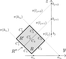
Figure 7. Replacing $R$, $R^{\prime}$ with their union $R^{\prime\prime}$

Proof.

To prove each statement, we need to show that CCD structure and all the conclusions in Theorem 1.4 are preserved after changing $\Delta_{N}$ the way described in the statement.

To prove (1), let $P^{(1)},\dots,P^{(m)}$ be the separate components of $P$. After putting the corresponding separate components of $L$ into appropriate positions (without changing their contact type) in $(\mathbb{R}^{3},\xi_{0})$, we may assume that the projection

$$P=P^{(1)}\cup\dots\cup P^{(m)}$$

of $L$ onto the second quadrant of the $yz$-plane is given similar as the one which we illustrated in Figure 8.

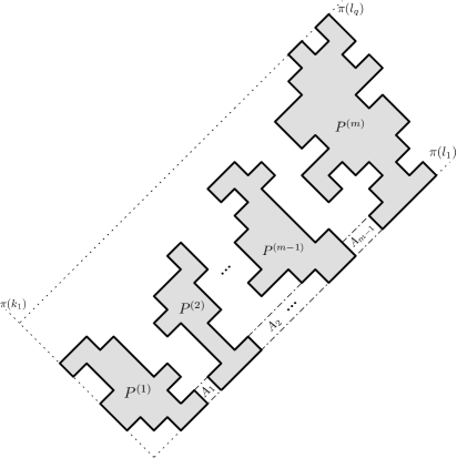
Figure 8. Modifying the algorithm for the case when $L$ is split

In such a projection, we require two important properties:

1. $P^{(1)},\dots,P^{(m)}$ are located from left to right in the given order in the region bounded by the lines $\pi(k_{1})$, $\pi(l_{1})$, and $\pi(l_{q})$.

2. Each of $P^{(1)},\dots,P^{(m)}$ has at least one edge on the line $\pi(l_{1})$.

If the components $P^{(1)}\dots P^{(m)}$ remain separate, then our construction in Theorem 1.4 cannot work (the complement of the union of 3-cells corresponding to the rectangles in $P$ would not be a Darboux ball; it would be a genus $m$ handle body). So we have to make sure that any component $P^{(l)}$ is connected to the some other via some bridge consisting of rectangles. We choose only one rectangle for each bridge as follows: Let $A_{l}$ be the rectangle in $T_{1}$ (the row between $\pi(l_{1})$ and $\pi(l_{2})$) connecting $P^{(l)}$ to $P^{(l+1)}$ for $l=1,\dots,m-1$ (see Figure 8). Now, by adding 2- and 3-cells (corresponding to $A_{1},\dots,A_{m-1}$), we can extend the CCD $\Delta_{N}$ to get another CCD for $(S^{3},\xi_{st})$. Therefore, we have modified our construction when $L$ is split.

To prove (2), if we replace $D^{\prime\prime}$ in the way described above, then by the construction of $\Delta_{N}^{3}$, we also replace two 3-cells with a single 3-cell whose boundary is the union of $D^{\prime\prime}$ and its isotopic copy. This alteration of $\Delta_{N}^{3}$ does not change the fact that the boundary of the union of all 3-cells coming from all pairs of saddle disks is still homeomorphic to a 2-sphere $S^{2}$, Therefore, we can still complete this union to $S^{3}$ by gluing a complementary Darboux ball. Thus, we still have a CCD. Note that $\gamma\cap\gamma^{\prime}$ is taken away from the 1-skeleton. However, since $L\cap\gamma\cap\gamma^{\prime}=\emptyset$, the new 1-skeleton still contains $L$. Observe also that this process does not change the ribbon $N(L)$ of $L$. Hence, the same conclusions in Theorem 1.4 are satisfied by the new CCD. ∎

4. Examples

Example I. As the first example, let us finish the one which we have already started in the previous section. Consider the Legendrian right trefoil knot $L$ (Figure 1) and the corresponding region $P$ given in Figure 5. Then we construct the 1-skeleton, the saddle disks, and the ribbon of the CCD $\Delta$ as in Figure 9.

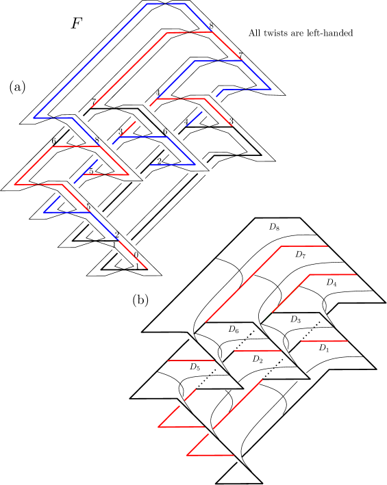
Figure 9. (a) The page $F$ for the right trefoil knot, (b) Construction of $\Delta$

In Figure 9-(a), we show how to construct the 1-skeleton $G=\Delta^{1}$ of $\Delta$ starting from a single Legendrian arc (labelled by the number “ 0 ”). We add Legendrian arcs labelled by the pairs of numbers “$1,1$”$,\dots,$“$8,8$” to the picture one by one (in this order). Each pair determines the endpoints of the corresponding arc. These arcs represent the cores of the 1-handles building the page $F$ (the ribbon of $G$) of the corresponding open book $\mathcal{OB}$. Note that by attaching each 1-handle, we (positively) stabilize the previous ribbon by the positive Hopf band $(H^{+}_{k},t_{\gamma_{k}})$ where $\gamma_{k}$ is the boundary of the saddle disk $D_{k}$ as before. Therefore, the monodromy $h$ of $\mathcal{OB}$ supporting $(S^{3},\xi_{st})$ is given by

$$h=t_{\gamma_{1}}\circ\dots\circ t_{\gamma_{8}}$$

where $t_{\gamma_{k}}\in Aut(F,\partial F)$ denotes the positive (right-handed) Dehn twist along $\gamma_{k}$. To compute the genus $g_{F}$ of $F$, observe that $F$ is constructed by attaching eight 1-handles (bands) to a disk, and $|\partial F|=3$ where $|\partial F|$ is the number of boundary components of $F$. Therefore,

$$\chi(F)=1-8=2-2g_{F}-|\partial F|\Longrightarrow g_{F}=3.$$

Now suppose that $(M_{1}^{\pm},\xi^{\pm}_{1})$ is obtained by performing contact $(\pm 1)$-surgery on $L$. Clearly, the trefoil knot $L$ sits as a Legendrian curve on $F$ by our construction, so by Theorem 2.5, we get the open book $(F,h_{1})$ supporting $\xi$ with monodromy

$$h_{1}=t_{\gamma_{1}}\circ\dots\circ t_{\gamma_{8}}\circ t_{L}^{\mp 1}\in Aut(F,\partial F).$$

Hence, we get an upper bound for the support genus invariant of $\xi_{1}$, namely,

$$sg(\xi_{1})\leq 3=g_{F}.$$

We note that the upper bound, which we can get for this particular case, from [AO] and [St] is $6$ where the page of the open book is the Seifert surface $F_{5,5}$ of the $(5,5)$-torus link (see Figure 10).

Figure 10. Legendrian right trefoil knot sitting on $F_{5,5}$

Example II. Consider the Legendrian figure-eight knot $L$, and its square bridge position given in Figure 11-(a) and (b). We get the corresponding region $P$ in Figure 11-(c). Using Remark 3.2 we replace $R_{5}$ and $R_{8}$ with a single saddle disk. So this changes the set $\mathfrak{P}$. Reindexing the rectangles in $\mathfrak{P}$, we get the decomposition in Figure 12 which will be used to construct the CCD $\Delta$.

Figure 11. (a),(b) Legendrian figure-eight knot, (c) The region $P$

Figure 12. Modifying the region $P$

In Figure 13-(a), similar to Example I, we construct the 1-skeleton $G=\Delta^{1}$ of $\Delta$ again by attaching Legendrian arcs (labelled by the pairs of numbers “$1,1$”$,\dots,$ “$10,10$”) to the initial arc (labelled by the number “0”) in the given order. Again each pair determines the endpoints of the corresponding arc, and the cores of the 1-handles building the page $F$ (of the corresponding open book $\mathcal{OB}$). Once again attaching each 1-handle is equivalent to (positively) stabilizing the previous ribbon by the positive Hopf band $(H^{+}_{k},t_{\gamma_{k}})$ for $k=1,\dots,10$. Therefore, the monodromy $h$ of $\mathcal{OB}$ supporting $(S^{3},\xi_{st})$ is given by

$$h=t_{\gamma_{1}}\circ\dots\circ t_{\gamma_{10}}$$

To compute the genus $g_{F}$ of $F$, observe that $F$ is constructed by attaching ten 1-handles (bands) to a disk, and $|\partial F|=5$. Therefore,

$$\chi(F)=1-10=2-2g_{F}-|\partial F|\Longrightarrow g_{F}=3.$$

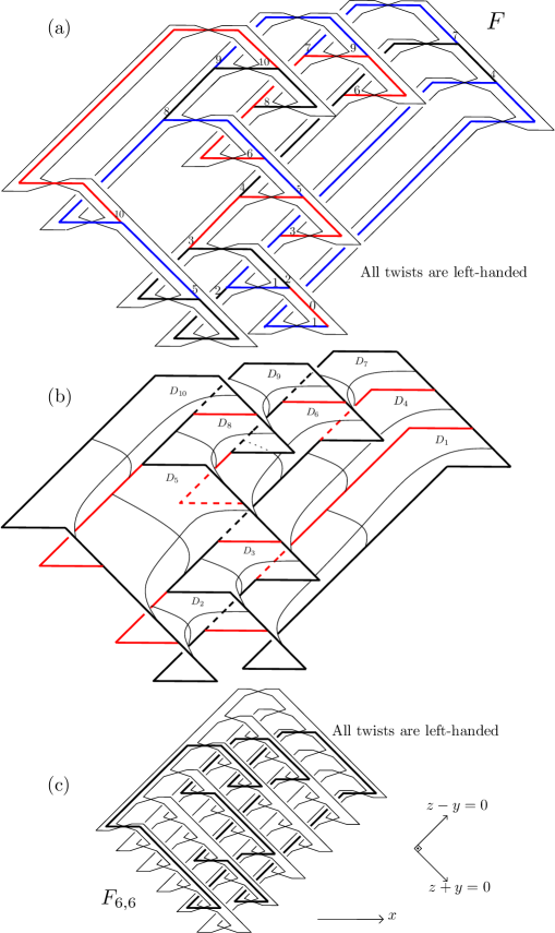
Figure 13. (a) The page $F$, (b) Construction of $\Delta$, (c) The figure-eight knot on $F_{6,6}$

Let $(M_{2}^{\pm},\xi^{\pm}_{2})$ be a contact manifold obtained by performing contact $(\pm)$-surgery on the figure-8 knot $L$. Since $L$ sits as a Legendrian curve on $F$ by our construction, Theorem 2.5 gives an open book $(F,h_{2})$ supporting $\xi_{2}$ with monodromy

$$h_{2}=t_{\gamma_{1}}\circ\dots\circ t_{\gamma_{10}}\circ t_{L}^{\mp 1}\in Aut(F,\partial F).$$

Therefore, we get the upper bound $sg(\xi_{2})\leq 3=g_{F}$. Once again we note that the smallest possible upper bound, which we can get for this particular case, using the method of [AO] and [St] is $10$ where the page of the open book is the Seifert surface $F_{6,6}$ of the $(6,6)$-torus link (see Figure 13-(c)).

References

- [AO] S. Akbulut, B. Ozbagci, Lefschetz fibrations on compact Stein surfaces, Geom. Topol. 5 (2001), 319–334 (electronic).
- [DG1] F. Ding and H. Geiges, A Legendrian surgery presentation of contact -manifolds, Math. Proc. Cambridge Philos. Soc. 136 (2004), no. 3, 583–598.
- [Et1] J. B. Etnyre, Planar open book decompositions and contact structures, IMRN 79 (2004), 4255–4267.
- [Et2] J. B. Etnyre, Lectures on open book decompositions and contact structures, Floer homology, gauge theory, and low-dimensional topology, 103–141, Clay Math. Proc., 5, Amer. Math. Soc., Providence, RI, 2006.
- [Et3] J. Etnyre, Introductory Lectures on Contact Geometry, Topology and geometry of manifolds (Athens, GA, 2001), 81–107, Proc. Sympos. Pure Math., 71, Amer. Math. Soc., Providence, RI, 2003.
- [EO] J. Etnyre, and B. Ozbagci, Invariants of Contact Structures from Open Books, arXiv:math.GT/0605441, preprint 2006.
- [Ga] D. Gabai, Detecting fibred links in , Comment. Math. Helv., 61(4):519-555, 1986.
- [Ge] H. Geiges, Contact geometry, Handbook of differential geometry. Vol. II, 315–382, Elsevier/North-Holland, Amsterdam, 2006.
- [Gd] N Goodman, Contact Structures and Open Books, PhD thesis, University of Texas at Austin (2003)
- [Gi] E. Giroux, Géométrie de contact: de la dimension trois vers les dimensions supérieures, Proceedings of the ICM, Beijing 2002, vol. 2, 405–414.
- [Gm] R. E. Gompf, Handlebody construction of Stein surfaces, Ann. of Math. 148 (1998), 619–693.
- [GS] R. E. Gompf, A. I. Stipsicz, 4-manifolds and Kirby calculus, Graduate Studies in Math. 20, Amer. Math. Soc., Providence, RI, 1999.
- [Ho] K. Honda, On the classification of tight contact structures -I, Geom. Topol. 4 (2000), 309–368 (electronic).
- [LP] A. Loi, R. Piergallini, Compact Stein surfaces with boundary as branched covers of , Invent. Math. 143 (2001), 325–348.
- [Ly] H. Lyon, Torus knots in the complements of links and surfaces, Michigan Math. J. 27 (1980), 39-46.
- [OS] B. Ozbagci, A. I. Stipsicz, Surgery on contact 3-manifolds and Stein surfaces, Bolyai Society Mathematical Studies, 13 (2004), Springer-Verlag, Berlin.
- [Pl] O. Plamenevskaya, Contact structures with distinct Heegaard Floer invariants, Math. Res. Lett., 11 (2004), 547-561.
- [St] A. I. Stipsicz, Surgery diagrams and open book decomposition of contact 3-manifolds, Acta Math. Hungar, 108 (1-2) (2005), 71-86.
- [TW] W. P. Thurston, H. E. Winkelnkemper, On the existence of contact forms, Proc. Amer. Math. Soc. 52 (1975), 345–347.