Gravitating Global k-monopole

Abstract

A gravitating global k-monopole produces a tiny gravitational field outside the core in addition to a solid angular deficit in the k-field theory. As a new feature, the gravitational field can be attractive or repulsive depending on the non-canonical kinetic term.

1 Introduction

The phase transition in the early universe could produce different kinds of topological defects which have some important implications in cosmology[1]. Domain walls are two-dimensional defects, and strings are one-dimensional defects. Point-like defects also arise in same theories which undergo the spontaneous symmetry breaking, and they appears as monopoles. The global monopole, which has divergent mass in flat spacetime, is one of the most interesting defects. The idea that monopoles ought to exist has been proved to be remarkably durable. Barriola and Vilenkin [2] firstly researched the characteristic of global monopole in curved spacetime, or equivalently, its gravitational effects. When one considers the gravity, the linearly divergent mass of global monopole has an effect analogous to that of a deficit solid angle plus that of a tiny mass at the origin. Harari and Loustò [3], and Shi and Li [4] have shown that this small gravitational potential is actually repulsive. Furthermore, Li et al [5, 6, 7] have proposed a new class of cold stars which are called D-stars (defect stars). One of the most important features of such stars, comparing to Q-stars, is that the theory has monopole solutions when the matter field is absent, which makes the D-stars behave very differently from the Q-stars. The topological defects are also investigated in the Friedmann-Robertson-Walker spacetime [8]. It is shown that the properties of global monopoles in asymptotically dS/AdS spacetime [9] and the Brans-Dicke theory [10] are very different from those of ordinary ones. The similar issue for the gravitational mass of composite monopole, i.e., global and local monopole has also been discussed [22].

The huge attractive force between global monopole $M$ and antimonopole $\bar{M}$ proposes that the monopole over-production problem does not exist, because the pair annihilation is very efficient. Barriola and Vilenkin have shown that the radiative lifetime of the pair is very short as they lose energy by Goldstone boson radiation [2]. No serious attempt has made to develop an analytical model of the cosmological evolution of a global monopole, so we are limited to the numerical simulations of evolution by Bennett and Rhie [11]. In the $\sigma$-model approximation, the average number of monopoles per horizon is $N_{H}\sim 4$. The gravitational field of global monopoles can lead to clustering in matter, and later evolve into galaxies and clusters. The scale-invariant spectrum of fluctuations has been given [11]. Furthermore, one can numerically obtain the microwave background anisotropy $(\delta T/T)_{\rm rms}$ patterns [12]. Comparing theoretical value to the observed rms fluctuation, one can find the constraint of parameters in global monopole.

On the other hand, non-canonical kinetic terms are rather ordinary for effective field theories. The k-field theory, in which the non-canonical kinetic terms are introduced in the Lagrangian, have been recently investigated to serve as the inflaton in the inflation scenario, which is so-called k-inflation [13], and to explain the current acceleration of the universe and the cosmic coincidence problem, k-essence [14]. Armendariz-Picon et al [15, 16] have discussed gravitationally bound static and spherically symmetric configurations of k-essence fields. Another interesting application of k-fields is topological defects, dubbed by k-defects [17]. Monopole [18] and vortex [19] of tachyon field, which as an example of k-field comes from string/M theory, have also been investigated. The mass of global k-monopole diverges in flat spacetime, just as that of standard global monopole, therefore, it is of more physical significance to consider the gravitational effects of global k-monopole.

In this paper, we study the gravitational field of global k-monopole and derive the solutions numerically and asymptotically. We find that the topological condition of vacuum manifold for the formation of a k-monopole is identical to that of an ordinary monopole, but their physical properties are disparate. Especially, we show that the mass of k-monopole can be positive in some form of the non-canonical kinetic terms. In other words, the gravitational field can be attractive or repulsive depending on the non-canonical kinetic term.

2 Equations of Motion

We shall work within a particular model in units $c=1$, where a global $O(3)$ symmetry is broken down to $U(1)$ in the k-field theory. Its action is given by

$$S=\frac{1}{2\kappa}\int d^{4}\tilde{x}\sqrt{-g}\left[M^{4}K(\tilde{X}/M^{4})-\frac{1}{4}\lambda^{2}(\tilde{\phi}^{a}\tilde{\phi}^{a}-\tilde{\sigma}_{0}^{2})^{2}\right],$$ (1)

where $\kappa=8\pi G$ and $\lambda$ is a dimensionless constant. In action (1), $\tilde{X}=\frac{1}{2}\left(\tilde{\partial}_{\mu}\tilde{\phi}^{a}\tilde{\partial}^{\mu}\tilde{\phi}^{a}\right)$, where $\tilde{\phi}^{a}$ is the $SO(3)$ triplet of goldstone field and $\tilde{\sigma}_{0}$ is the symmetry breaking scale with a dimension of mass. After setting the dimensionless quantities: $x=M\tilde{x}$, $\phi_{a}=\tilde{\phi}_{a}/M$ and $\sigma_{0}=\tilde{\sigma}_{0}/M$, action (1) becomes

$$S=\frac{1}{2\kappa}\int d^{4}x\sqrt{-g}\left[K(X)-V(\phi)\right],$$ (2)

where $V(\phi)=\frac{1}{4}\lambda^{2}(\phi^{a}\phi^{a}-\sigma_{0}^{2})^{2}$. The hedgedog configuration describing a global k-monopole is

$$\phi^{a}=\sigma_{0}f(\rho)\frac{x^{a}}{\rho},$$ (3)

where $x^{a}x^{a}=\rho^{2}$ and $a=1,2,3$, so that we shall actually have a global k-monopole solution if $f\rightarrow 1$ at spatial infinity and $f\rightarrow 0$ near the origin.

The static spherically symmetric metric can be written as

$$ds^{2}=B(\rho)dt^{2}-A(\rho)d\rho^{2}-\rho^{2}(d\theta^{2}+\sin^{2}\theta d\varphi^{2})$$ (4)

with the usual relation between the spherical coordinates $\rho$, $\theta$, $\varphi$ and the ”Cartesian” coordinate $x^{a}$. Introducing a dimensionless parameter $r=\sigma_{0}\rho$, from (2) and (3), we obtain the equations of motion for $f$ as

$$\dot{K}\left\{\frac{1}{A}f^{\prime\prime}+\left[\frac{2}{Ar}+\frac{1}{2B}\left(\frac{B}{A}\right)^{\prime}\right]f^{\prime}-\frac{2}{r^{2}}f\right\}+\ddot{K}\frac{X^{\prime}f^{\prime}}{A}-\lambda^{2}f(f^{2}-1)=0,$$ (5)

where the prime denotes the derivative with respect to $r$, the dot denotes the derivative with respect to $X$ and $X=-\frac{f^{2}}{r^{2}}-\frac{f^{\prime 2}}{2A}$. Since we only consider the static solution, positive $X$ and negative $X$ are irrelevant each other. In this paper, we will assume $K(X)$ to be valid for negative $X$.

The Einstein equation for k-monopole is

$$G_{\mu\nu}=\kappa T_{\mu\nu}$$ (6)

where $T_{\mu\nu}$ is the energy-momentum tensor for the action (2). The tt and rr components of the Einstein equations now could be written as

$$-\frac{1}{A}\left(\frac{1}{r^{2}}-\frac{1}{r}\frac{A^{\prime}}{A}\right)+\frac{1}{r^{2}} = \epsilon^{2}T^{0}_{0}$$ (7)

$$-\frac{1}{A}\left(\frac{1}{r^{2}}+\frac{1}{r}\frac{B^{\prime}}{B}\right)+\frac{1}{r^{2}} = \epsilon^{2}T^{1}_{1},$$ (8)

where

$$T^{0}_{0} = -K+\frac{\lambda^{2}}{4}(f^{2}-1)^{2}$$ (9)

$$T^{1}_{1} = -K+\frac{\lambda^{2}}{4}(f^{2}-1)^{2}-\dot{K}\frac{f^{\prime 2}}{A}$$ (10)

and $\epsilon^{2}=\kappa\sigma_{0}^{2}=8\pi G\sigma_{0}^{2}$ is a dimensionless parameter.

3 k-monopole

Although the existence of global k-monopole, as well as the standard one, is guaranteed by the symmetry-breaking potential, there exist the non-canonical kinetic term in k-monopole which certainly leads to the appearance of a new scale in the action and the mass parameter in the potential term. However, the non-canonical kinetic term is non-trivial. At small gradients, it can be chosen to have a same asymptotical behavior with that of the standard one, so that it ensures the standard manner of a small perturbations. While at large gradient we choose it to have a different form from the standard one.

In the small $X$ case, we assume that the kinetic term has the asymptotically canonical behavior, which can avoid ”zero-kinetic problem”. If $|X|\ll 1$, we have $K(X)\sim X^{\alpha}$, and $\alpha<1$ then there is a singularity at $X=0$; and $\alpha>1$ then the system becomes non-dynamical at $X=0$. For the monopole solution, it is easily found that $K(X)\sim X$ at $r\gg 1$. On the other hand, we assume that the modificatory kinetic term $K(X)\sim X^{\alpha}$ and $\alpha\neq 1$ at $|X|\gg 1$. One can easily obtain the equation of motion inside the core of a global monopole after assuming that $|X|\gg 1$ in the core of the global monopole. The equations of motion are highly non-linear and cannot be solved analytically. Next, we investigate the asymptotic behaviors of global monopole with non-linear in $X$ kinetic term. To be specific, we consider the following type of kinetic term

$$K(X)=X-\beta X^{2},$$ (11)

where $\beta$ is a parameter of global k-monopole. It is easy to find that global k-monopole will reduce to be the standard one when $\beta=0$. It is easy to check whether the kinetic term (11) satisfy the condition for the hyperbolicity [16, 20, 17]

$$\frac{\dot{K}}{2X\ddot{K}+\dot{K}}>0,$$ (12)

which leads to a positive definite speed of sound for the small perturbations of the field. The stability of solutions shows that for the case $\beta<0$, the range $\frac{1}{6\beta}>X>\frac{1}{2\beta}$ must be excluded. However, this will not destroy the results which are carried out from the case $\beta>0$. We here only consider the cases for $\beta>0$.

Using Eqs.(5)-(10), we get the asymptotic expression for $A(r)$, $B(r)$, and $f(r)$ which is valid near $r=0$,

$$f(r) = f_{0}{r}+\frac{{f_{0}}\,\left[2\,\lambda^{2}\,\left(-3+\epsilon^{2}\right)++42\beta\,\epsilon^{2}\,{{f_{0}}}^{4}\right]}{60\,\left(1+5\beta\,{{f_{0}}}^{2}\right)}{r}^{3}$$

$$+ \frac{f_{0}\left[\left(9+7\beta\,\lambda^{2}\right)\,\epsilon^{2}\,{{f_{0}}}^{2}+36\beta^{2}\,\epsilon^{2}\,{{f_{0}}}^{6}\right]}{60\,\left(1+5\beta\,{{f_{0}}}^{2}\right)}{r}^{3}+O(r^{4})$$

$$A(r)=1+\frac{\epsilon^{2}\,\left(\lambda^{2}+6\,{{f_{0}}}^{2}+9\beta\,{{f_{0}}}^{4}\right)}{12}{r}^{2}+O(r^{3})$$ (14)

$$B(r)=1+\frac{\epsilon^{2}\,\left(\lambda^{2}-9\beta\,{{f_{0}}}^{4}\right)}{12}{r}^{2}+O(r^{3}),$$ (15)

where the undetermined coefficient $f_{0}$ is characterized as the mass of k-monopole, which can be determined in the numerical calculation.

In the region of $r\gg 1$, similarly we can expand $f(r)$, $A(r)$ and $B(r)$ as

$$f(r) = 1-\frac{1}{\lambda^{2}}\left(\frac{1}{r}\right)^{2}-\frac{3-2\,\epsilon^{2}+4\beta\,\lambda^{2}}{2\,{\lambda^{4}}}\left(\frac{1}{r}\right)^{4}+O(r^{-5})$$ (16)

$$A(r) = \frac{1}{1-\epsilon^{2}}-\frac{{M_{\infty}}}{{(1-\epsilon^{2})^{2}}}\frac{1}{r}+\left[\frac{\epsilon^{2}(1-\beta\lambda^{2})}{{\left(1-\epsilon^{2}\right)}^{2}\,\lambda^{2}}+\frac{{M_{\infty}^{2}}}{{(1-\epsilon^{2})^{3}}}\right]\left(\frac{1}{r}\right)^{2}$$

$$+ O(r^{-3})$$

$$B(r) = (1-\epsilon^{2})+M_{\infty}\frac{1}{r}-\frac{\epsilon^{2}\,\left(1-\beta\lambda^{2}\right)}{\lambda^{2}}\left(\frac{1}{r}\right)^{2}+O(r^{-3}),$$ (18)

where the constant $M_{\infty}$ will be discussed in the following.

Using shooting method for boundary value problems, we get the numerical results of the function $f(r)$ which describes the configuration of global k-monopole. In Fig.1 we show the function $f(r)$ for $\beta=0$, $\beta=1$, $\beta=5$ and $\beta=10$ respectively and for given values of $\lambda$ and $\epsilon$. Obviously, the configuration of field $f$ is not impressible to the choice of the parameter $\beta$.

Figure 1: The plot of $f(r)$ as a function of $r$. Here we choose $\lambda=1$, $G=1$ and $\epsilon=0.001$. The four curved lines are plotted when $\beta=0$, $\beta=1$, $\beta=5$ and $\beta=10$ respectively.

From Eqs.(3) and (16), it is easy to construct global k-monopole which has the same asymptotic condition with standard global monopole, i.e., $f$ will approach to zero when $r\ll 1$ and approach to unity when $r\gg 1$.

Actually there is a general solution to Einstein equation with energy-momentum tensor $T_{\mu\nu}$ which takes the form as (9) and (10) for spherically symmetric metric (4)

$$A(r)^{-1}=1-\frac{\epsilon^{2}}{r}\int_{0}^{r}[-K+\frac{\lambda^{2}}{4}(f^{2}-1)^{2}]r^{2}dr$$ (19)

$$B(r)=A(r)^{-1}\exp\left[\epsilon^{2}\int_{\infty}^{r}(\dot{K}{f^{\prime 2}}r)dr\right].$$ (20)

In terms of the dimensionless quantity $\epsilon$, the metric coefficient $A(r)$ and $B(r)$ can be formally integrated and read as

$$A(r)^{-1}=1-\epsilon^{2}-\frac{2G\sigma_{0}M_{A}(r)}{r}$$ (21)

$$B(r)=1-\epsilon^{2}-\frac{2G\sigma_{0}M_{B}(r)}{r}.$$ (22)

The small dimensionless parameter $\epsilon$ arise naturally from Einstein equations and clearly $\epsilon^{2}$ describes a solid angular deficit of space-time.

A global k-monopole solution $f$ should approach unity when $r\gg 1$. If this convergence is fast enough, then $M_{A}(r)$ and $M_{B}(r)$ will also rapidly converge to finite values. Therefore, from Eqs.(16)-(18) we have the asymptotic expansions:

$$M_{A}(r) = {M_{\infty}}+4\pi\sigma_{0}\,\left(-\beta+\frac{1}{{\lambda}^{2}}\right)\frac{1}{r}+\frac{8\pi\sigma_{0}\left(-1+\epsilon^{2}+2\,\beta\,{\lambda}^{2}\right)}{3\,{\lambda}^{4}}\left(\frac{1}{r}\right)^{3}$$

$$+ O(r^{-5})$$

$$M_{B}(r) = {M_{\infty}}+4\pi\sigma_{0}\,\left(-\beta+\frac{1}{{\lambda}^{2}}\right)\frac{1}{r}-\frac{4\pi\sigma_{0}\,\left(-1+\epsilon^{2}-4\,\beta\,{\lambda}^{2}\right)}{3\,{\lambda}^{4}}\left(\frac{1}{r}\right)^{3}$$

$$+ O(r^{-5}),$$

where $M_{\infty}\equiv\lim_{r\rightarrow\infty}M_{A}(r)$. One can easily find that the dependence on $\epsilon$ of the asymptotic expansion for $f(r)$ is very weak, in other words, the asymptotic behavior is quite independent of the scale of symmetry breakdown $\sigma_{0}$ up to value as large as the planck scale. On the contrary, $M_{A}(r)$ depends obviously on $\sigma_{0}$.

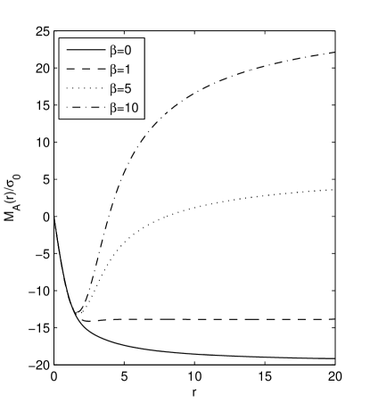
Figure 2: The plot of $M_{A}(r)/\sigma_{0}$ as a function of $r$. Here we choose $\lambda=1$, $G=1$ and $\epsilon=0.001$. The four curved lines are plotted when $\beta=0$, $\beta=1$, $\beta=5$ and $\beta=10$ respectively.

The numerical results of $M_{A}(r)/\sigma_{0}$ are shown in Fig.2 by shooting method for boundary value problems where we choose $\lambda=1$, $G=1$ and $\epsilon=0.001$. From the figure, we find that the mass of global k-monopole decrease to a negative asymptotic value when $r$ approaches infinity in the case that $\beta=0$ and $\beta=1$. While the mass will be positive if $\beta=5$ or $\beta=10$. The asymptotic mass for the cases above are $-19.15\sigma_{0}$, $-13.83\sigma_{0}$, $3.62\sigma_{0}$ and $22.14\sigma_{0}$ respectively. It is clear that the presence of parameter $\beta$, which measures the degree of deviation of kinetic term from canonical one, affects the effective mass of the global k-monopole significantly. It is not difficult to understand this property. From Eqs.(11), (19) and (21), the mass function $M_{A}(r)$ can be expressed explicitly as

$$\frac{M_{A}(r)}{4\pi\sigma_{0}}=-r+\int_{0}^{r}\left[\beta X^{2}-X+\frac{\lambda^{2}}{4}(f^{2}-1)^{2}\right]r^{2}dr.$$ (25)

Obviously, the $\beta$-term in the integration has the positive contribution for the mass function. From Fig.1, $f$ (then $X$) is not sensitive to the value of $\beta$, so the greater parameter $\beta$ is chosen, the larger value $M_{A}(r)$ takes for a given $r$, and if $\beta$ is greater than some value, $M_{A}(r)$ will be positive for large $r$ as Fig.2 shows. However, inside the core, $X$ varies slowly but $f$ varies fast with respect to $r$, therefore, $\lambda^{2}$-term in the integration will become dominant as $r$ decreases. This leads to two characteristics of the mass curves which is also shown in Fig.2: (i) the mass curves with different $\beta$ converge gradually in the region near $r=0$; (ii) in the case that $\beta$ is large enough, $M_{A}(r)$ has a minimum.

To show the effect of solid defect angle, we then investigate the motion test particles around a global k-monopole. It is a good approximation to take $M_{A}(r)$ as a constant in the region far away from the core of the global k-monopole, since the the mass $M_{A}(r)$ approaches very quickly to its asymptotic value. Therefore, we can consider the geodesic equation in the metric (4) with

$$A(r)^{-1}=B(r)=1-\epsilon^{2}-\frac{2GM}{r}$$ (26)

where $M=\sigma_{0}M_{\infty}$. Solving the geodesic equation and introducing a dimensionless quantaty $u=GM/r$, one will get the second order differentiating equation of $u$ with respect to $\varphi$ [9, 21]

$$\frac{d^{2}u}{d\varphi^{2}}+(1-\epsilon^{2})u=\left(\frac{GM}{L}\right)^{2}+3u^{2},$$ (27)

where $L$ is the angular momentum per unit of mass. When $\left(\frac{GM}{L}\right)^{2}\varphi\ll 1$, one have the approximate solution of $u$

$$u\approx\left(\frac{GM}{L}\right)^{2}\left\{\frac{1}{1-\epsilon^{2}}+e\cos\left[\left(1-\frac{3}{\sqrt{\left(1-\epsilon^{2}\right)^{3}}}\left(\frac{GM}{L}\right)^{2}\right)\varphi\right]\right\},$$ (28)

where $e$ denotes the eccentricity. When a test particle rotates one loop around the global k-monopole, the precession of it will be

$$\Delta\varphi=6\pi\left(\frac{GM}{L}\right)^{2}\frac{1}{\sqrt{\left(1-\epsilon^{2}\right)^{3}}}\approx 6\pi\left(\frac{GM}{L}\right)^{2}+9\pi\left(\frac{GM}{L}\right)^{2}\epsilon^{2}.$$ (29)

The last term in Eq.(29) is the modificaiton comparing this result with that for the precession around an ordinary star.

4 Conclusion

In summary, k-monopole could arise during the phase transition in the early universe. We calculate the asymptotic solutions of global k-monopole in static spherically symmetric spacetime, and find that the behavior of a k-monopole is similar to that of a standard one. Although the choice of the parameter $\beta$, which measures the degree of deviation of kinetic term from canonical one, have little influence on the configuration of k-field $\phi$, the effective mass of global k-monopole is affected significantly. The mass might be negative or positive when different parameters $\beta$ are chosen. This shows that the gravitational field of the global k-monopole could be attractive or repulsive depending on the different non-canonical kinetic term.

The configuration of a global k-monopole is more complicated than that of a standard one. As for its cosmological evolution, we should not attempt to get the analytical mode, instead we can only use numerical simulation. However, the energy dominance of global k-monopole is in the region outside the core. We can roughly estimate that global k-monopoles will result in the clustering in matter and evolve into galaxies and clusters in a way similar to that of standard monopoles.

References

References

- [1] Vilenkin A and Shellard E P S, 1994 Cosmic Strings and Other Topological Defects (Cambridge Unversity Press, Cambridge, England)
- [2] Barriola M and Vilenkin A, 1989 Phys. Rev. Lett. 63, 341
- [3] Harari D and Loustò C, 1990 Phys. Rev.D42, 2626
- [4] Shi X and Li X Z, 1991 Class. Quantum Grav. 8, 761
- [5] Li X Z and Zhai X H, 1995 Phys. Lett. B364, 212
- [6] Li J M and Li X Z, 1998 Chin. Phys. Lett.15, 3; Li X Z, Liu D J and Hao J G, 2002 Science in China A45, 520
- [7] Li X Z, Zhai X H and Chen G, 2000 Astropart. Phys. 13, 245
- [8] Basu R, Guth A H and Vilenkin A, 1991 Phys. Rev. D44 340; Basu R and Vilenkin A, 1994 Phys. Rev. D50 7150; Chen C, Cheng H, Li X Z and Zhai X H, 1996 Class. Quantum Grav. 13, 701
- [9] Li X Z and Hao J G, 2002 Phys. Rev. D66, 107701; Hao J G and Li X Z, 2003 Class. Quantum Grav. 20, 1703
- [10] Li X Z and Lu J Z, 2000 Phys. Rev. D62, 107501
- [11] Bennett D P and Rhie S H, 1990 Phys. Rev. Lett. 65, 1709
- [12] Bennett D P and Rhie S H, 1993 Astrophys. J. 406, L7
- [13] Armendariz-Picon C, Damour T, Mukhanov V, 1999 Phys.Lett. B458, 209
- [14] Armendariz-Picon C, Mukhanov V, Steinhardt P J, 2000 Phys.Rev.Lett.85, 4438; Armendariz-Picon C, Mukhanov V, Steinhardt P J, 2001 Phys. Rev. D63: 103510
- [15] Armendariz-Picon C and Lim E A, 2005 JCAP 0508, 007
- [16] Bilic N, Tupper G B and Viollier R D, 2006 JCAP 0602 013; Diez-Tejedor A and Feinstein A, 2006 Phys. Rev. D74 023530; Nucamendi U, Salgado M and Sudarsky D, 2000 Phys. Rev. Lett. 84 3037; Nucamendi U, Salgado M and Sudarsky D, 2001 Phys. Rev. D63 125016.
- [17] Babichev E, 2006 Phys. Rev. D74 085004
- [18] Li X Z and Liu D J, 2005 Int. J. Mod. Phys. A20, 5491
- [19] Liu D J and Li X Z, 2003 Chin. Phys. Lett. 20, 1678
- [20] Rendall A D, 2006 Class.Quant.Grav. 23, 1557.
- [21] Wald R M, 1984 General Ralitivity (The university of Chicago Press, Chicago)
- [22] Spinelly J, de Freitas U and Bezerra de Mello E R, 2002 Phys.Rev. D66, 024018.