¹⁰Li spectrum from ¹¹Li fragmentation.

Abstract

A recently developed time dependent model for the excitation of a nucleon from a bound state to a continuum resonant state in the system n+core is applied to the study of the population of the low energy continuum of the unbound ¹⁰Li system obtained from ¹¹Li fragmentation. Comparison of the model results to new data from the GSI laboratory suggests that the reaction mechanism is dominated by final state effects rather than by the sudden process, but for the population of the l=0 virtual state, in which case the two mechanisms give almost identical results. There is also, for the first time, a clear evidence for the population of a d_5/2 resonance in ¹⁰Li.

1 Introduction

In this paper we apply the projectile fragmentation model developped in Ref. [1] to the the elastic breakup (diffraction reaction) of the two-neutron halo nucleus ¹¹Li on a ¹²C target, as recently measured at GSI and presented in Ref. [2]. The observable studied is the one-neutron-core relative energy spectrum. These type of data are necessary to enlighten the effect of the neutron final state interaction with the core of origin.

Light unbound nuclei have attracted much attention [3]-[48] in connection with exotic halo nuclei. Besides, a precise understanding of unbound nuclei is essential to determine the position of the driplines in the nuclear mass chart. In two-neutron halo nuclei such as ⁶He, ¹¹Li, ¹⁴Be, the two neutron pair is bound, although weakly, due to the neutron-neutron pairing force, while each single extra neutron is unbound in the field of the core. In a three-body model these nuclei are described as a core plus two neutrons. The properties of the core plus one neutron system are essential to structure models which rely on the knowledge of single particle quantum numbers such as angular momentum, parity, energies, as well as the corresponding neutron-core effective potential. With those ingredients the spectroscopic strength function of neutron resonances in the field of the core can be obtained.

We will use the projectile fragmentation formalism, an inelastic-like excitation to the neutron-core continuum, to the study of the effect of final state interaction of the neutron with the projectile core. The model is a theory which has already been shown to be relevant to the interpretation of neutron-core coincidence measurements in nuclear elastic breakup reactions with projectiles of ¹⁴B and ¹⁴Be [1, 2]. In the case of two nucleon breakup we describe only the step in which a neutron is knocked out from the projectile by the neutron-target interaction to first order and then re-interacts in the final state with the core. The case in which a resonance is populated by a sudden process while the other neutron is stripped has been already discussed in Ref. [3] and it has been shown [1] that there is a simple link between the two methods of Ref. [1] and Ref.[3]. We assume that the neutron which is not detected has been stripped while the other suffers an elastic scattering on the target. The influence of the second nucleon is taken into account only by a modification of the neutron-core interaction in the final state. Section 2 contains a brief reminder of the formalism from Ref. [1]. Section 3 describes the results of our numerical calculations for ¹¹Li which, being already well understood [2]-[24], is used here as a test case. Details on our assumptions for the potentials needed in the calculations are also presented. Finally our conclusions are contained in Sec. 4.

2 Formalism for inelastic excitation to the continuum.

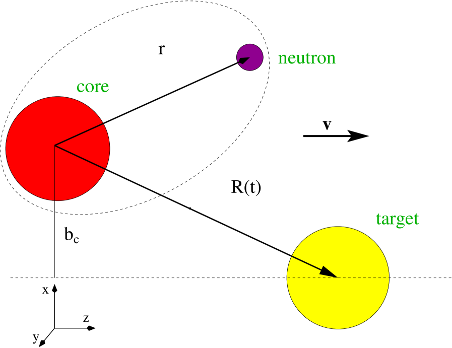
Figure 1: Coordinate system used in the calculations

Following Refs. [1, 50, 51, 52], we will describe the inelastic-like excitations of one neutron, from a bound state $\psi_{i}$ to a final state $\psi_{f}$ in the continuum, by the time dependent perturbation amplitude :

$$A_{fi}={1\over i\hbar}\int_{-\infty}^{\infty}dt\langle\psi_{f}({\bf r},t)|V_{2}({\bf{r-R}}(t))|\psi_{i}({\bf r},t)\rangle.$$ (1)

$V_{2}$ is the interaction responsible for the neutron transition (cf. Eq. (2.15) of [50]). The potential $V_{2}({\bf{r-R}}(t))$ moves past on a constant velocity path with velocity $v$ in the z-direction with an impact parameter $b_{c}$ in the x-direction in the plane $y=0$. This assumption makes our semiclassical model valid at beam energies well above the Coulomb barrier. This is in fact the regime in which projectile fragmentation experiments are usually performed (cf. Sec. 3). The coordinate system used in the calculations is shown in Fig. 1 and it corresponds to the no-recoil approximation for the core. Let $\psi_{i}({\bf r},t)=\phi_{i}({\bf r})e^{-{i\over\hbar}\varepsilon_{i}t}$ be the single particle initial state wave function. Its radial part $\phi_{i}({\bf r})$ is calculated in a potential $V_{WS}(r)$ (cf. Sec. 3.1) which is fixed in space. For initial and final states of different angular momentum our wave functions are trivially orthogonal due to the orthonormality of their angular parts. For transitions conserving the angular momentum of the single particle states the orthogonalization correction has been estimated in Ref. [1] and found negligible. Now change variables and put $z-vt=z^{\prime}$ or $t=(z-z^{\prime})/v$, define

$$q={{\varepsilon_{f}-\varepsilon_{i}}\over{\hbar v}},$$ (2)

then choosing $V_{2}(r)$ to be a delta-function potential $V_{2}(r)=v_{2}\delta(x)\delta(y)\delta(z)$, with $v_{2}\equiv$ [MeV fm³], the integrals over x and y can be calculated giving

$$A_{fi}={v_{2}\over i\hbar v}\int_{-\infty}^{\infty}dz~{}\phi^{*}_{f}(b_{c},0,z)\phi_{i}(b_{c},0,z){e^{iqz}}.$$ (3)

The value of the strength $v_{2}$ used in the calculation is discussed in Sec. 3.

The following forms for the wave functions will be used. For the initial bound state

$$\phi_{i}({\bf r})=-C_{i}i^{l_{i}}\gamma h^{(1)}_{l_{i}}(i\gamma r)Y_{{l_{i}},{m_{i}}}(\theta,\phi).$$ (4)

Due of the strong core absorption implied in the following by Eq. (8), we use in this paper the asymptotic form of the initial state wave function, given in terms of the Hankel functions $h^{(1)}_{l}$. However the exact wave function, numerical solution of the bound state Schrödinger equation can be used without introducing further complexity in the calculations. For the final continuum state

$$\phi_{f}({\bf r})=C_{f}k{i\over 2}(h^{(-)}_{l_{f}}(kr)-S_{l_{f}}h^{(+)}_{l_{f}}(kr))Y_{{l_{f}},{m_{f}}}(\theta,\phi),$$ (5)

$C_{f}=\sqrt{2/L}$ is the normalization constant for the final state. L is a large box radius used to normalize the continuum wave function (cf. Eq. (2.5) of Ref. [49]). $S_{l_{f}}=e^{2i\delta_{l_{f}}}$ is the neutron-target S-matrix in the $l_{f}$ partial wave.

The probability to excite a final continuum state of energy $\varepsilon_{f}$ is an average over the initial state and a sum over the final states. Thus introducing the density of final states and the density of final states, according to Ref. [49] $\rho(\varepsilon_{f})d\varepsilon_{f}={Lm/\pi\hbar^{2}k}d\varepsilon_{f},$ the probability spectrum reads

$${dP_{in}\over d\varepsilon_{f}}={2\over\pi}{v_{2}^{2}\over\hbar^{2}v^{2}}{C_{i}^{2}}{m\over\hbar^{2}k}{1\over 2l_{i}+1}\Sigma_{m_{i},m_{f}}|1-\bar{S}_{m_{i},m_{f}}|^{2}|I_{m_{i},m_{f}}|^{2},$$ (6)

where now $\bar{S}=Se^{2i\nu}=e^{2i(\delta+\nu)}$ is an off-the-energy shell S-matrix and $\nu$ is the phase of the integral:

$$I_{m_{i},m_{f}}=\int_{-\infty}^{\infty}dze^{iqz}i^{l_{i}}\gamma h^{(1)}_{l_{i}}(i\gamma r)Y_{{l_{i}},{m_{i}}}(\theta,0)k{i\over 2}h^{(-)}_{l_{f}}(kr)Y_{{l_{f}},{m_{f}}}(\theta,0).$$ (7)

A detailed derivation of the above equations can be found in Sec.2 of Ref. [1]. For simplicity the equations in this paper are given without spin variables in the initial and final states. The generalization including spin is given in Appendix B of Ref. [1].

The cross section differential in $\varepsilon_{f}$ is given as

$${d\sigma_{-1n}\over{d{{\varepsilon_{f}}}}}=C^{2}S\int d{\bf b_{c}}{dP_{in}(b_{c})\over d{{\varepsilon_{f}}}}P_{ct}(b_{c}),$$ (8)

(see Eq. (2.3) of [53]) and C²S is the spectroscopic factor for the initial state.

The core survival probability $P_{ct}(b_{c})=|S_{ct}|^{2}$ [53] in Eq. (8) takes into account the peripheral nature of the reaction and naturally excludes the possibility of large overlaps between projectile and target. $P_{ct}$ is defined in terms of a S-matrix function of the core-target distance of closest approach $b_{c}$. A simple parameterisation is $P_{ct}(b_{c})=e^{(-\ln 2exp[(R_{s}-b_{c})/a])}$ [53], where the strong absorption radius R${}_{s}\approx 1.4(A_{p}^{1/3}+A_{t}^{1/3})$ fm is defined as the distance of closest approach for a trajectory that is 50% absorbed from the elastic channel and a=0.6 fm is a diffuseness parameter.

3 Applications

3.1 One neutron average potential

We apply the fragmentation model to the study of the relative energy spectrum n+⁹Li obtained by the authors of Ref. [2] in the breakup reaction of ¹¹Li on ¹²C at 264 A.MeV. The structure of ¹¹Li is already well known from a number of experiments and theoretical papers [2]-[24]: the two neutron separation energy is 0.3$\pm$0.27 MeV [54]; the wave function is combination of a 2s state with a spectroscopic factor 0.31, a p_1/2 with spectroscopic factor 0.45 [4] and there is also a small d_5/2 component. The main d_5/2 strength is in the continuum centered around 1.55 MeV [2]. The link between reaction theory and structure model is made by the neutron-core potential determining the S-matrix in Eq. (5). Then if the theory fits the position and shape of the continuum n-nucleus energy distribution, obtained for example by a coincidence measurement between the neutron and the core, the parameters of a model potential can be deduced.

The calculations in the present paper are made with different potentials for the initial and final state. The initial wave function for the s-state is calculated in a simple Woods-Saxon potential with R= r${}_{0}A^{1/3}$ and strength fitted to the separation energy 0.3 MeV[54] and whose parameters are given in Table 1.

$$V_{WS}(r)={V_{0}\over{1+e^{(r-R)/a}}}-\left({\hbar\over m_{\pi}c}\right)^{2}{V_{so}\over ar}{e^{(r-R)/a}\over{(1+e^{(r-R)/a})^{2}}}{\mathbf{l\cdot\sigma}}$$ (9)

Table 1: Asymptotic normalization constants C_i(fm^-1/2) for the initial state components wave functions of the bound neutron. Spectroscopic factors from Ref. [4]. Potential parameters are: V₀ fitted to give the separation energy 0.3 MeV [54]. The other potential parameters are r₀=1.27 fm, a=0.75 fm, V_so=5.25 MeV.

$\varepsilon_{i}$	-0.3 MeV
$l_{i},~{}~{}j_{i}$	Ci(fm-1/2)	C2S
0 $~{}~{}{1/2}$	0.76	0.31
1 $~{}~{}{1/2}$	0.24	0.45

Table 2: Woods-Saxon and spin-orbit potential parameters for the continuum final states.

V0	r0	a	Vso	aso
(MeV)	(fm)	(fm)	(MeV)	(fm)
-39.8	1.27	0.75	7.07	0.75

To describe the valence neutron in the ¹⁰Li continuum we assume that the single neutron hamiltonian with respect to ⁹Li has the form

$$h=t+U+iW$$ (10)

where $t$ is the kinetic energy and

$$U(r)=V_{WS}+\delta V$$ (11)

is the real part of the neutron-core interaction. In this paper the imaginary part is taken equal to zero. V_WS is again a Woods-Saxon potential plus spin-orbit whose parameters are given in Table 2, and $\delta$V is a correction [17]:

$$\delta V(r)=16\alpha{e^{{{2(r-R)}/a}}/({1+e^{{{(r-R)}/a}}})^{4}}$$ (12)

which originates from particle-vibration couplings. They are important for low energy states but can be neglected at higher energies. The above form is suggested by a calculation of such couplings using Bohr and Mottelson collective model of the transition amplitudes between zero and one phonon states. Therefore our structure model is not a simple single-particle in a potential model but contains in it the full complexity of single-particle vs. collective couplings. A more realistic treatment would require the description of both bound and unbound states in a three-body model such as in Refs. [46] and [47].

The continuum energies can be adjusted by varying the parameter $\alpha$ in the potential. By changing the strength $\alpha$ of the $\delta$V potential in Eq. (12) we could make also the 2s-state just bound near threshold and see what would be the effect on the continuum spectrum (cf.[1, 8]). As possible final states we have considered only the s, p and d partial waves calculated in the potential of Table 2 plus Eq. (12), according to Ref. [17], with different values of the strength $\alpha$. Table 3 gives the energies and widths of the 1p_1/2 and 1d_5/2 states and the corresponding values of $\alpha$. The widths are obtained from the phase shift variation near resonance energy, according to $d\delta_{j}/d\varepsilon_{f}|_{\varepsilon_{res}}=2/\Gamma_{j}$, once that the resonance energy is fixed [55]. Notice that the values of $\alpha$ for the s and d states are very similar, therefore these two states are basically obtained in the same potential.

Table 3: Scattering length of the 2s continuum state, energies and widths of the p- and d-resonances in ¹⁰Li and corresponding strength parameters for the $\delta$V potential.

		$\varepsilon_{res}$	$\Gamma_{j}$	as	$\alpha$
		MeV	MeV	fm-1	MeV
	2s1/2			-17.2	-10.0
	1p1/2	0.63	0.35		3.3
	1d5/2	1.55	0.18		-9.8

The delta-interaction strength used in Eq. (6), is $v_{2}$=-8625 MeV fm³. It has been obtained by imposing that this interaction gives the same volume integral as a n-¹²C Woods-Saxon potential of strength -50.5MeV, radius 2.9 fm and diffuseness 0.75 fm.

3.2 Results

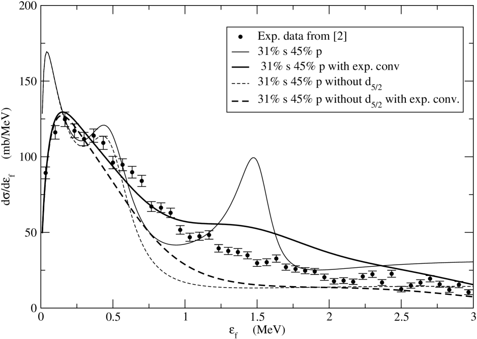
Figure 2: n-⁹Li relative energy spectrum, for the reaction ¹¹Li+¹²C $\to$ n+⁹Li+X at 264 A.MeV. Only the contributions from an s and p initial state with experimental spectroscopic factors [4] C²S= 0.31 and 0.45 respectively are included. The thin solid curve is the total calculated result. The thick solid curve curve is after convolution with the experimental resolution function. The thin dashed curve is the calculation without the d-resonance while the thick dashed curve is the same calculation after convolution. The symbols with error bars are the experimental points from [2]. Calculations are normalised to the data.

Figure 3: The individual transitions, bound to unbound from the s and p initial state components, taken with unit spectroscopic factors, to the s,p and d unbound state as indicated. The thick dashed line is the sum of all transitions, including the spectroscopic factors for the initial state components while the thick solid line is does not include transitions to the d-resonance.

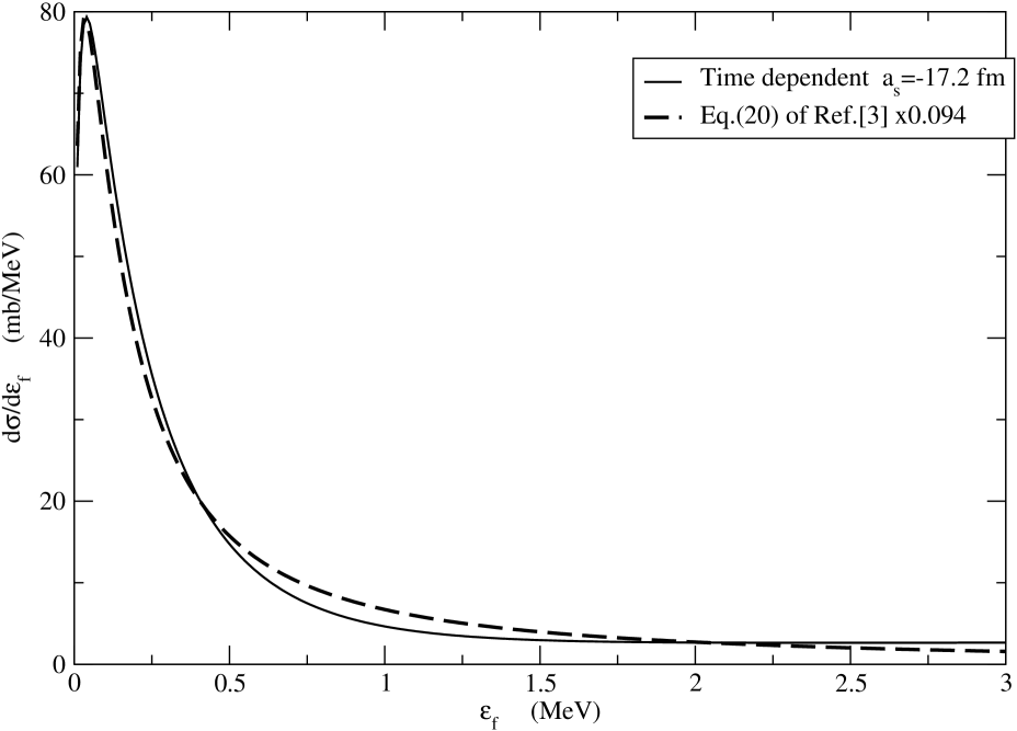
Figure 4: Comparison for the s to s transition of our calculation (solid curve) with that according to the sudden formula Eq. (20) of [3]. Both calculations use the exact phase shifts.

Results obtained with the model outlined in Secs. 2 and 3.1 will now be discussed. We consider the knockout of a single neutron from a bound state in a potential, similarly to the previous calculation for ¹¹Be, ¹⁴Be and ¹⁴B [1]. The reaction corresponds to a neutron initially bound in ¹¹Li which is then excited into an unbound state of ¹⁰Li, assuming that another nucleon has been emitted and stripped by the target, thus not detected in coincidence with the core. One of the results of Ref. [1], as far as the reaction model is concerned, was to show that projectile fragmentation invariant mass spectra depend very weakly on the incident energy and on the neutron initial binding energy. Related to this was the investigation of the validity of the sudden approximation and the accuracy necessary in calculating the phase shifts.

In Fig. 2 the symbols with error bars are the experimental points from [2]. The thin full curve is the calculated total spectrum, sum of the contributions from the s and p components of the initial wave function, with the parameters of Table 1 and the experimental spectroscopic factors from Ref. [4]. Using the theoretical spectroscopic factors from Refs. [16], [17] gives very small differences in the shape of the total spectrum which however become unnoticeable after convolution with the experimental resolution function. The s, p and d final continuum states have the parameters of Table 3. Notice that these parameters are perfectly consistent with those extracted from the data and given by Table 4 of Ref. [2]. The thick solid curve is the same calculation after convolution with the experimental resolution function. The dashed curve is the calculation without the d-resonance after convolution while the thin dashed curve is the bare calculation without the d-resonance contribution. The agreement between the thick solid curve and the data is quite good and it shows the importance of including the d-resonance to reproduce the tail of the experimental spectrum. The Coulomb breakup spectrum from the s component of the initial state was also calculated but since it gives a contribution of less than 5% to the peak of the spectrum, it has been omitted from the figures.

The individual transitions, bound to unbound from each initial state component to each possible unbound state as indicated, are shown in Fig. 3. We give also in Fig. 4 the comparison for the s to s transition of our calculation with the calculation according to the sudden formula Eq. (20) of [3] which we discussed at length and compared to our model in Ref. [1]. Both calculations were done with the exact phase shift, obtained by solving numerically the Schrödinger equation with the potential given by Eqs. (11,12). Contrary to what it was found in Ref. [1] for ¹³Be, we find here that in the case of the ¹⁰Li virtual state, the scattering length is large enough, i.e. the state is close enough to threshold, to justify the use of the sudden approximation. Furthermore we have checked that the effective range formula (cf. discussion after Eq. (41) of Ref. [1]) gives in this case a very good fit to the exact phase shift. In fact, using it in Eq. (20) of [3] gives a curve almost indistinguishable from the dashed line in Fig. 4. The parameters obtained from the fit are: a_s=-14.8 fm, r_e= 7.5 fm. Notice that the scattering length value obtained instead as a_s=-$\lim_{k\to 0}{\delta_{0}\over k}$ and given in Table 3 was -17.2 fm. This is the kind of sensitivity one can find using the two different prescriptions for a_s. On the other hand we have checked that the value of r_e from the fit, is consistent with the behaviour of our continuum state potential, Eqs. (11,12). Such potential becomes indeed negligible, and consistent with zero, for r$>$r_e= 7.5 fm, as prescribed for the applicability of the effective range theory.

As already found in Ref. [1] for ¹¹Be and ¹³Be, we can confirm here with the ¹⁰Li example that, a part for the s to s transition, the excitation of resonances with $l>0$ in the continuum of unbound nuclei in projectile fragmentation reactions, is a final state effect due to n-core interaction, rather than a process in which a bound component of the initial wave function becomes suddenly unbound. The results in Fig. 3 show clearly that the population of continuum resonance is dominated by the contributions from the s-initial state, while the transitions p to p or p to d are not large enough to explain the experimental spectrum. This is particularly clear for the d-resonance whose presence is necessary to explain the experimental spectrum tail but whose strength could not be justified by a d to d transition which would have a very small amplitude. Therefore the strength of the continuum resonances of a daughter nucleus does not reflect directly the occupation of the bound states of same angular momentum in the mother nucleus. This is different from the common wisdom on the breakup of two-neutron halo nuclei, as discussed for example in the recent Ref. [7].

In the case of ¹¹Li the two neutrons are in the same state for each component of the initial wave function. Therefore since the p and d wave functions have less pronounced tails, the stripping probability of one of the two neutrons, as discussed in Sec. 3 of Ref. [1], will naturally diminish the absolute value of the peaks due to transitions from these states, with respect to peaks due to transition from the bound s-component. This effect is not taken into account at the moment in our numerical implementations of the model. On the other hand our absolute cross sections should be multiplied by a factor two to take into account the fact that the experimental data do not distinguish the two neutrons in the continuum. The absolute value of our cross section can be read from the dashed curve in Fig. 3. Taking into account the factor two just mentioned, we see that in order to compare to the experimental data in Fig. 2, which are given on their absolute scale, we still have to renormalise our calculations by a factor two. Considering the incertitude in the value of the neutron-target delta-interaction potential and in the strong absorption radius, we can consider our estimates quite reasonable.

4 Conclusions and outlook

In this paper we have studied the energy spectrum of ¹⁰Li as obtained from the fragmentation of ¹¹Li by applying a model [1] for one neutron excitations from a bound initial state to an unbound resonant state in the neutron-core low energy continuum. The model, based on a time dependent perturbation theory amplitude, was previously used [1] to study ¹³Be and the breakup of ¹¹Be and it proved to be reliable. The same conclusion can be drawn here after comparing our calculations with the new data from [2].

The initial state spectroscopic factors in ¹¹Li are quite well known experimentally, therefore the absolute values of our cross sections have also been checked, besides the shape of the n-core relative energy spectrum. Due to the closeness to threshold of the s virtual state we have seen that the sudden formula used in Ref. [3] and the effective range approximation to the phase shift, are both very well justified for ¹⁰Li, contrary to what it was previously [1] found for ¹³Be. Finally we have found that, in agreement with the interpretation given by the authors of [2], their recent data provide a clear evidence on the excitation of a d resonance around 1.5 MeV. Such a resonance does not play much role in the composition of the ¹¹Li ground state but it is an important building bloc of its excited states.

Acknowledgments

We wish to thank Björn Jonson and his collaborators, in particular Leonid Chulkov and Haik Simon, for communicating their results previous to publication and for an enlightening correspondence.

References

- [1] G. Blanchon, A. Bonaccorso, D.M. Brink, A. García-Camacho and N. Vinh Mau. Nucl. Phys. A784 (2007) 49.
- [2] H. Simon, M. Meister , T. Aumann, M.J.G. Borge, L.V. Chulkov , U. Datta Pramanik, Th.W. Elzeh, H. Emling, C. Forss en, H. Geissel, M. Hellstr om, B. Jonson, J. V. Kratz, R. Kulessa, Y. Leifels, K. Markenroth, G. M unzenberg, F. Nickel, T. Nilsson, G. Nyman, A. Richter, K. Riisager, C. Scheidenberger, G. Schrieder, O. Tengblad and M. V. Zhukov, Systematic investigation of the drip-line nuclei 11Li and 14Be and their unbound subsystems 10Li and 13Be, To be published in NPA.
- [3] G. F. Bertsch, K. Hencken and H. Esbensen, Phys. Rev. C57 (1998) 1366.
- [4] S. N. Ershov et al., Phys. Rev. C70 (2004) 054608.
- [5] T. Nakamura et al., Phys. Rev. Lett. 96 (2006) 252502.
- [6] D.R. Tilley, J.H. Kelley, J.L. Godwin, D.J. Millener, J.E. Purcell, C.G. Sheu and H.R. Weller, Nucl. Phys. A745 (2004)155.
- [7] I. Brida, F.M. Nunes and B.A. Brown, Nucl. Phys. A775 ( 2006) 23.
- [8] G. Blanchon, A. Bonaccorso and N. Vinh Mau, Nucl. Phys. A739 (2004) 259.
- [9] B. Jonson, Phys. Rep. 389 (2004) 1.
- [10] M. Zinser et al., Nucl. Phys. A619 (1997) 151.
- [11] S. Pita, Thesis University Paris 6 (2000), IPN Orsay IPNO-T-00-11. S. Fortier, Proc. Int. Symposium on Exotic Nuclear Structures ENS 2000, Debrecen (Hungary), Heavy Ion Physics 12 (2001) 255.
- [12] M. Chartier et al., Phys. Lett. B510 (2001) 24.
- [13] P. Santi, Ph. D. thesis, University of Notre Dame, (2000), unpublished. P. Santi et al., Phys. Rev. C67 (2003) 024606.
- [14] H. B. Jeppesen for the ISOLDE and REX-ISOLDE collaboration, Nucl. Phys. A 748, (2005) 374. H.B. Jeppesen et al., Phys. Lett. B 642 ( 2006) 449.
- [15] G. F. Bertsch and H. Esbensen, Ann. Phys. (N.Y.) 209 (1991) 327.
- [16] I. J. Thompson and M. V. Zhukov, Phys. Rev. C53 (1996) 708.
- [17] N. Vinh Mau and J. C. Pacheco, Nucl. Phys. A607 (1996) 163.
- [18] J. C. Pacheco and N. Vinh Mau, Phys. Rev. C65 044004 (2002).
- [19] N. Vinh Mau, Nucl. Phys. A592 (1995) 33.
- [20] G. Colò, T. Suzuki and H. Sagawa, Nucl. Phys. A695 (2001) 167.
- [21] E. Garrido, D. V. Fedorov, A. S. Jensen, Nucl. Phys. A708 (2002) 277 and references therein.
- [22] T. Myo, S.Aoyama ,K. Kato and K. Ikeda, Phys. Lett. B576 (2003) 281.
- [23] I. J. Thompson and M. V. Zukhov, Phys. Rev. C49 (1994) 1904.
- [24] A. Bonaccorso and N. Vinh Mau, Nucl. Phys. A615 (1997) 245.
- [25] J. L. Lecouey, Ph. D. thesis, University of Caen, (2002), unpublished and nucl-ex/0310027.
- [26] M. Thoennessen, Proceedings the International School of Heavy-Ion Physics, 4th Course: Exotic Nuclei, Erice, May 1997, Eds. R. A. Broglia and P. G. Hansen, (World Scientific, Singapore 1998), pag.269.
- [27] M. Labiche et al. Phys. Rev. Lett. 86 (2001) 600.
- [28] M. Thoennessen et al., Phys. Rev. C59 (1999) 111.
- [29] M. Thoennessen, S. Yokoyama, and P.G. Hansen, Phys. Rev. C60 (1999) 027303.
- [30] H. Simon et al., Nucl. Phys. A734 (2004) 323.
- [31] L. V. Chulkov et al, Phys. Rev. Lett. 79 (1997) 201. L. V. Chulkov and G. Schrieder, Z. Phys. A359 (1997) 231. D. V. Aleksandrov et al., Nucl. Phys. A669 (2000) 51 and references therein.
- [32] D.V. Aleksandrov et al., Sov. J. Nucl. Phys. 37(3) (1983).
- [33] H. G. Bohlen et al. Nucl. Phys. A616 (1997) 254c.
- [34] J. A. Caggiano et al., Phys. Rev. C60 (1999) 064322.
- [35] B. M. Young et al. Phys. Rev. C49 (1994) 279.
- [36] A. N. Ostrowski et al., Z. Phys. A343 (1992) 489.
- [37] A. V. Belozyorov et al., Nucl. Phys. A636 (1998) 419; Phys. Rev. C63 (2000) 014308.
- [38] A. A. Korsheninnikov et al., Phys. Lett. B343 (1995) 53.
- [39] S. Fortier et al., Phys. Lett. B461 (1999) 22 ; T. Aumann et al., Phys. Rev. Lett. 84 (2000) 35 and references therein.
- [40] J. Margueron, A. Bonaccorso and D. M. Brink, Nucl. Phys. A720 (2003) 337.
- [41] P. Capel, D. Baye, Phys. Rev. C70 (2004) 064605.
- [42] P. Descouvemont, Phys. Lett. B331 (1994) 271.
- [43] P. Descouvemont, Phys. Rev. C52 (1995) 704.
- [44] A. Adachour, D. Baye and P. Descouvemont, Phys. Lett. B356 (1995) 445
- [45] D. Baye, Nucl. Phys. A627 (1997) 305.
- [46] M. Rodriguez-Gallardo et al, Phys. Rev. C72, (2005) 024007.
- [47] I. J. Thompson et al, Phys. Rev. C47, (1993) R1364.
- [48] M. Labiche, F. M. Marques, O. Sorlin, and N. Vinh Mau, Phys. Rev. C60 (1999) 027303.
- [49] A. Bonaccorso and D. M. Brink, Phys. Rev. C38 (1988) 1776.
- [50] A. Bonaccorso and D. M. Brink, Phys. Rev. C43 (1991) 299.
- [51] K. Adler, A. Bohr, T.Huus, B. Mottelson and A. Winther, Rev. Mod. Phys. 28 (1956) 432. K. Alder and A. Winther, Electromagnetic Excitation (North-Holland, Amsterdam, 1975).
- [52] R. A. Broglia, and A. Winther, , Addison-Wesley Publ., Redwood City, CA. 1991. Ch.V.
- [53] A. Bonaccorso, Phys. Rev. C60 (1999) 054604.
- [54] http://nucleardata.nuclear.lu.se/database/masses/
- [55] C. J. Joachain, Quantum Collision Theory, North-Holland Publishing Company, Amsterdam-Oxford, 1975.