A Way to Dynamically Overcome the Cosmological Constant Problem

Abstract

The Cosmological Constant problem can be solved once we require that the full standard Einstein Hilbert lagrangian, gravity plus matter, is multiplied by a total derivative. We analyze such a picture writing the total derivative as the covariant gradient of a new vector field ($b_{\mu}$). The dynamics of this $b_{\mu}$ field can play a key role in the explanation of the present cosmological acceleration of the Universe.

I Introduction.

There are numerous suggestions in the literature for modification of the classical Einstein Hilbert (EH) eqs of motion of general relativity ($G_{\mu\nu}\equiv R_{\mu\nu}-\frac{g_{\mu\nu}}{2}R=T_{\mu\nu}/m_{Pl}^{2}$) in connection with the solution of the Cosmological Constant (CC) problem weinb ,CC . Many approaches concentrate their attention on possible modifications of the the world volume ($\int d^{4}x\sqrt{g}$), in particular, we will briefly review the main features of Unimodular Gravity and Two Measure Theory (TMT) whose features are most similar to our findings.

In unimodular gravity, see uni , the salient point is the non dynamical character of the determinant of the metric tensor $g=det||g_{\alpha\beta}||$ that is frozen to a constant value, leaving a theory invariant only under volume preserving general coordinate transformations unimodular . In absence of matter the action can be written as

$$S_{Un}=\int d^{4}x\sqrt{g}\,\,(\,R+\Lambda)+\lambda(g-1)\;$$ (1)

where $\lambda$ is a lagrange multiplier that fix the constraint $g=1$ and $\Lambda$ the CC. The unimodular eqs of motion are

$$R_{\mu\nu}-\frac{1}{4}g_{\mu\nu}R=0\rightarrow\nabla_{\mu}R=0$$ (2)

where there is no trace of the initial $\Lambda$ CC; however the solution remains of DeSitter type: $R_{\mu\nu}=\frac{1}{4}\;g_{\mu\nu}\;\Lambda^{\prime}$ with $\Lambda^{\prime}=const$ a new CC different from the original one ($\Lambda$), coming from the boundary conditions of eqs (2) (the same conclusions are obtained in presence of matter). This, strictly speaking, does not solve the problem of the CC but it changes the perspective and allows one to think of the CC as a non dynamical entity.

An other interesting approach is the Two Measure Theory, introduced and fully developed by Guendelman and Kaganovich gk . In this case the action is of the form

$$S=\int d^{4}x\;\Phi\;{\cal L}_{1}+\int d^{4}x\;\sqrt{g}\;{\cal L}_{2}$$ (3)

with two lagrangians ${\cal L}_{1,2}$ functions of all matter fields, the metric, the connection (the theory is defined in first order Palatini formalism) and two different volume elements ($\sqrt{g}\,d^{4}x$ and $\Phi\,d^{4}x$) where $\Phi$ is a scalar density:

$$\Phi=\epsilon^{\mu\nu\rho\sigma}\epsilon_{abcd}\partial_{\mu}\phi_{a}\partial_{\nu}\phi_{b}\partial_{\rho}\phi_{c}\partial_{\sigma}\phi_{d}$$ (4)

that results a total derivative of the four fundamentals $\phi_{a}$ (a=1,2,3,4) scalar fields. The outcome of the extra measure is the presence of a new scalar field $\zeta=\frac{\Phi}{\sqrt{g}}$ which couple, after a conformal transformation, in a non trivial way to fermions and to an effective scalar potential that is automatically minimized into a state with zero CC without tuning of the parameters.

To our knowledge only few attempts to modify directly the structure of the world volume are present in literature, see for example wil and dc , also if somehow they are not devoted to the CC problem.

Now let us come to our proposal. The key ideas are based on basic properties: one is related to the covariant divergence of a vector field $b_{\mu}$: $\sqrt{g}\;\nabla^{\alpha}\;b_{\alpha}=\partial^{\alpha}(\sqrt{g}\;b_{\alpha})$ being a total derivative and the other is the fact that a shift in the total lagrangian ${\cal L}\rightarrow{\cal L}+\;const$ has no effect on the gravitational eqs of motion once we multiply everything by a total derivative. The combination of this two simple ideas can be summarized in the following non dynamical action:

$$\int d^{4}x\sqrt{g}\;\nabla_{\alpha}b^{\alpha}\;{\Lambda}={\Lambda}\int d^{4}x\;\partial_{\alpha}(\sqrt{g}\,\,b^{\alpha})=0$$ (5)

This motivate us to postulate that the total Lagrangian (including gravity and matter) $\bar{\cal L}$ of our world has to be multiplied by a total derivative

$$S=\int d^{4}x\;\sqrt{g}\;\;\nabla^{\alpha}b_{\alpha}\;\;\bar{\cal L}$$ (6)

in order to be automatically insensitive to any CC coming from the processes of renormalization or phase transitions. For the rest of the paper we use $\chi\equiv\nabla^{\alpha}b_{\alpha}$, having in mind the fact that we can introduce others total derivative terms as for example $\nabla^{2}\phi$ with $\phi$ a scalar field. The above postulate assumes implicitly that, if we start with a bare lagrangian $\bar{\cal L}_{0}$, the process of renormalization, generating the renormalized lagrangian $\bar{\cal L}$, with the corresponding CC $\Lambda$, conserves the original structure:

$$\int d^{4}x\sqrt{g}\;\;\chi\;\bar{\cal L}_{0}\!\!\!\!\!\!\!\!\!\!\underbrace{\Rightarrow}_{\rm Renormalization}\!\!\!\!\!\!\!\!\!\!\int d^{4}x\sqrt{g}\;\chi\;(\bar{\cal L}+\Lambda)$$ (7)

This result can be obtained if some symmetry principle can be worked out. We note, for example, that the full action is odd under the discrete symmetry $x_{\mu}\,\rightarrow-\,x_{\mu}$ for which $\chi\rightarrow-\chi$ , and $R\rightarrow R$. The matter lagrangian is naturally even for fields with an even power of derivatives (scalars and vectors) while, in order to accommodate also the fermionic fields which have only one derivative, we can ask also a non trivial transformation for the vierbien fields: $e^{\alpha}_{\mu}\,\rightarrow-\,e^{\alpha}_{\mu}$.

The above statements can be translated also in a postulated new modified world volume:

$$\int d^{4}x\;\sqrt{g}\rightarrow\int d^{4}x\;\sqrt{g}\;\chi$$ (8)

We note also that $\int d^{4}x\,\sqrt{g}\,\chi\,R$ cannot be modified in an Einstein form through a conformal transformation contrary to the case in which $\chi$ is a simple scalar field.

The subject of our analysis is the following action

$$S=\int d^{4}x\;\sqrt{g}\;\chi\;(m_{Pl}^{2}\;R-{\cal L})$$ (9)

where ${\cal L}\equiv{\cal L}_{m}+{\cal L}_{b}$ contains the usual matter Lagrangian ${\cal L}_{m}$ and the dynamics of the $b_{\mu}$ field (${\cal L}_{b}$).

We stress that many other scenarios can be implemented along the same lines, for instance $\int d^{4}x\sqrt{g}\;(\chi_{1}\,R-\chi_{2}\;{\cal L})$ with the presence (or the absence) of different $\chi_{i}$. We note that many formulas are comparables to the ones in the TMT gk also if the main assumptions result quite differents (for example our framework is a Riemannian geometry).

The eqs of motion from action (9) are:

• For the vector field :

  $$\nabla_{\mu}(m_{Pl}^{2}\,R\!-\!{\cal L})=\nabla^{\alpha}\!\left(\chi\frac{\partial{\cal L}_{b}}{\partial\nabla^{\alpha}b^{\mu}}\right)\!-\!\chi\frac{\partial{\cal L}_{b}}{\partial b^{\mu}}\equiv J_{\mu}^{(b)}$$ (10)

• For the matter fields ($\phi$):

  $$\nabla^{\alpha}\left(\frac{\partial{\cal L}_{m}}{\partial\nabla^{\alpha}\phi}\right)-\frac{\partial{\cal L}_{m}}{\partial\phi}=-\frac{\nabla^{\alpha}\chi}{\chi}\frac{\partial{\cal L}_{m}}{\partial\nabla^{\alpha}\phi}$$ (11)

• For gravity :

  $$\chi\, \left(m_{Pl}^{2}\,R_{\mu\nu}-\frac{\partial{\cal L}}{\partial g^{\mu\nu}}\right)=\frac{b_{\mu}J_{\nu}^{(b)}+b_{\nu}J_{\mu}^{(b)}}{2}-$$ (12)

  $$\frac{g_{\mu\nu}}{2}b^{\alpha}\,J_{\alpha}^{(b)}-m_{Pl}^{2}\left(g_{\mu\nu}\nabla^{2}-\nabla_{\mu}\nabla_{\nu}\right)\chi$$

where we used eq (10) to get rid of the terms $\nabla_{\nu}\left(m_{Pl}^{2}\,R-{\cal L}\right)$ as function of the current $J^{(b)}_{\mu}$. Eq (12) can be further simplified after the definition of the tensor

$$\tilde{T}_{\mu\nu}\equiv\frac{\partial{\cal L}}{\partial g^{\mu\nu}}$$ (13)

in the more usual form

$$m_{Pl}^{2} \left(R_{\mu\nu}\!-\frac{g_{\mu\nu}}{2}R\right)=\tilde{T}_{\mu\nu}-\frac{g_{\mu\nu}}{2}\tilde{T}+\frac{1}{2\,\chi}\left(b_{\mu}J_{\nu}^{(b)}+\right.$$ (14)

$$\left.b_{\nu}J_{\mu}^{(b)}\right)+\frac{m_{Pl}^{2}}{2\,\chi}\left(g_{\mu\nu}\nabla^{2}\!+2\,\,\nabla_{\mu}\,\nabla_{\nu}\right)\chi$$

that can also be rewritten in a compact form as

$$G_{\mu\nu}=\frac{1}{m_{Pl}^{2}}\left(T^{(m)eff}_{\mu\nu}+T^{(b)eff}_{\mu\nu}\right)$$ (15)

The $\tilde{T}_{\mu\nu}$ tensor being related to the usual energy momentum (EM) tensor by

$$T_{\mu\nu}\equiv\frac{\partial(\sqrt{g}{\cal L})}{\sqrt{g}\partial g^{\mu\nu}}=-\frac{g_{\mu\nu}}{2}\;{\cal L}+\tilde{T}_{\mu\nu}$$ (16)

allow us to write the new matter source of gravity as

$$T^{(m)eff}_{\mu\nu}\!\equiv\!\tilde{T}_{\mu\nu}^{(m)}\!-\!\frac{g_{\mu\nu}}{2}\tilde{T}^{(m)}\!=\!T_{\mu\nu}^{(m)}\!-\!\frac{g_{\mu\nu}}{2}(T^{(m)}+{\cal L}_{m})$$ (17)

while the vector field turn on the gravitational field by means of the tensor

$$T^{(b)eff}_{\mu\nu}\equiv \tilde{T}_{\mu\nu}^{(b)}-\frac{g_{\mu\nu}}{2}\tilde{T}^{(b)}+\frac{1}{2\,\chi}(b_{\mu}J_{\nu}^{(b)}+b_{\nu}J_{\mu}^{(b)})+$$ (18)

$$\frac{m_{Pl}^{2}}{2\,\chi}\left(\nabla^{2}\;g_{\mu\nu}+2\;\nabla_{\mu}\nabla_{\nu}\right)\chi$$

Finally we give the covariant conservation law for the matter EM tensor:

$$\nabla^{\alpha}T_{\mu\alpha}^{(m)}=-\tilde{T}_{\mu\alpha}^{(m)}\;\frac{\nabla^{\alpha}\;\chi}{\chi}$$ (19)

or in other terms: $\nabla^{\alpha}\left(T_{\mu\alpha}^{(m)}\,\chi\right)=-\frac{{\cal L}_{m}}{2}\nabla_{\mu}\chi$.

In order to be as simple as possible we take a vector lagrangian that depends separately on the combinations $\chi=\nabla^{\alpha}b_{\alpha}$ and $b^{2}=b^{\alpha}b_{\alpha}$ :

$${\cal L}_{b}=f(\chi)+U(b^{2})$$ (20)

with a vector current $J^{(b)}_{\mu}=\nabla_{\mu}(xf^{\prime})-2\,\chi\,U^{\prime}\,b_{\mu}$ and an effective EM tensor

$$T^{(b)eff}_{\mu\nu}=-\frac{g_{\mu\nu}}{2}\left(\chi\,f^{\prime}+U^{\prime}b^{2}\right)-U^{\prime}b_{\mu}b_{\nu}+$$ (21)

$$\frac{m_{Pl}^{2}}{2\,\chi}\left(\nabla^{2}\;g_{\mu\nu}+2\;\nabla_{\mu}\nabla_{\nu}\right)\chi$$

that inside eqs (10,11,12) generate the full dynamics of the system.

II Gravitational Sources

The new gravitational eqs (15) demand at this point some comments. The new sources of gravity, $T_{\mu\nu}^{(m)eff}+T_{\mu\nu}^{(b)eff}$, show strong departures from the structure of the classical EH sources ($T_{\mu\nu}^{(m)}+T_{\mu\nu}^{(b)}$).

Focusing only on matter, we note that the EM tensor is conserved once $\chi=const$ (see eq 19) and $T^{(m)eff}_{\mu\nu}$ reduces to $T^{(m)}_{\mu\nu}$ only when $g_{\mu\nu}\,(T^{(m)}+{\cal L}_{m})\ll T^{(m)}_{\mu\nu}$. The exact cancellation of this extra peace is a stringent condition on matter lagrangian gk

$$g^{\alpha\beta}\frac{\partial{\cal L}_{m}}{\partial g^{\alpha\beta}}-{\cal L}_{m}=0$$ (22)

which means that ${\cal L}_{m}$ is a homogeneous function of $g^{\alpha\beta}$ of degree one.

Other important aspect is the role played by different kinds of matter sources that we classify in two classes: the point particle ($pp$) and the coherent field ($cf$) configurations sources.

In general, both of them contribute to the dynamics of the system but the key point that will be elaborated in the following is the fact that point particle dynamics, contrary to coherent field configurations, has some freedom in his theoretical structure that allow us to obtain phenomenological viable matter sources.

II.1 Matter Point Particle Sources

The classical geodesic eqs for point particles extremize the functional $S_{pp}=\int d\tau\,{\cal L}_{pp}=-m\int d\tau\;\frac{ds}{d\tau}$, with $ds=\sqrt{g^{\alpha\beta}dx_{\alpha}x_{\beta}}$ the world element. The corresponding energy momentum tensor results $T_{\mu\nu}^{(pp)}=-\frac{1}{2}\int d\tau\,{\cal L}_{pp}\,v_{\mu}\,v_{\nu}$ (with $v_{\mu}\equiv\frac{dx_{\mu}}{d\tau}$). In this case the “anomalous” term counts $g_{\mu\nu}({\cal L}_{pp}+T^{(pp)})=-\frac{g_{\mu\nu}}{2}\int d\tau\,{\cal L}_{pp}$ and is never subdominant. The key point to evade such a non physical implication is the realization that for free point particles a full variety of actions are possible gk . The special property of the above $S_{pp}$ is reparametrization invariance but in general if, for example, we use a generalized action ${\cal S}_{pp}=-m\int d\tau F(\frac{ds}{d\tau})$ with $F(\frac{ds}{d\tau})$ a generic functional of the variable $(\frac{ds}{d\tau})$ and $\tau$ an affine parameter, in the EH context we generate the correct geodetic equations and the correct structure of the EM tensor. In our case instead, different choices of $F$ generate unequivalent theories. In fact now $T^{(pp)}_{\mu\nu}=\frac{m}{2}\int d\tau\;F^{\prime}\,v_{\mu}\,v_{\nu}$ and $g_{\mu\nu}({\cal L}_{pp}+T^{(pp)})=g_{\mu\nu}\;m\int d\tau\;(-F+\frac{F^{\prime}}{2})$ .

If we choose $F=\left(\frac{ds}{d\tau}\right)^{2}=g^{\alpha\beta}\frac{dx_{\alpha}}{d\tau}\frac{dx_{\beta}}{d\tau}$ we can get rid of the anomalous term gk and we obtain $T^{(pp)eff}_{\mu\nu}=T^{(pp)}_{\mu\nu}$ (note that now the $pp$ lagrangian is satisfying eq (22)). In this way the $pp$ dynamics coincides with the EH case.

II.2 Matter Coherent Field Sources

In order to work out the specific features of coherent field configurations we take a simple scalar field lagrangian

$${\cal L}_{m}=g^{\alpha\beta}\partial_{\alpha}\phi\partial_{\beta}\phi-V(\phi)$$

The effective EM tensor results:

$$T_{\mu\nu}^{eff(m)}=\partial_{\mu}\phi\partial_{\nu}\phi-\frac{g_{\mu\nu}}{2}(\partial\phi)^{2}=T_{\mu\nu}-\frac{g_{\mu\nu}}{2}V(\phi)$$ (23)

and the effective energy and pressure density in a FRW universe with a scale factor $a\equiv a(t)$ result

$$\rho_{m}^{eff}=\frac{\dot{\phi}^{2}}{2}+\langle\left(\frac{\vec{\nabla}\phi}{\sqrt{2}a}\right)^{2}\!\!\rangle,\;\;p_{m}^{eff}=\frac{\dot{\phi}^{2}}{2}-\langle\left(\frac{\vec{\nabla}\phi}{\sqrt{6}a}\right)^{2}\!\!\rangle$$ (24)

where an average $<...>$ over spatial gradients is imposed in order to preserve the spatial homogeneity.

The relationship between the usual eq of state $w=\frac{p}{\rho}$ and $w_{eff}=\frac{p_{eff}}{\rho_{eff}}$ during the various cosmological epochs is here synthesized

$$\underbrace{(-1,\,-\frac{1}{3},\,0,\,\frac{1}{3},\,1)}_{w}\leftrightarrow\underbrace{(Indef.\,,\,-\frac{1}{3},\,1,\,\frac{1}{3},\,1)}_{w_{eff}}$$ (25)

where we note as usual Inflationary phase ($w=-1$) cannot be generated with the new dynamics and the usual matter phase ($w=0$ with $\vec{\nabla}\phi=0$) of a classical oscillating coherent scalar field is now replaced by a faster kinetic phase. To evade such a conclusions it is in needed of a non trivial $g_{\alpha\beta}$ dependence in the interactions as it is the case for vector fields, like in the $b_{\mu}$ dynamics.

It is then clear that all the cosmological considerations related to the presence of dominant coherent fields ( like during the classical Inflationary period) have to be deeply reanalyzed.

III Vector Dynamics and CC

Now let us consider the vector field dynamics. What we discover is the fact that without interactions (in particular $U=0$) the system develops a CC completely unconstrained induced by the boundary conditions in a way similar to unimodular gravity. An appropriate choice of self interactions ($U\neq 0$) instead can dynamically constrain the system to calibrate his energy densities.

The key point is the vector eq (10) (see also eq (31)).

In the case with $U=0$ (or in general when $J^{(b)}_{\mu}$ is zero) eq (31) results a total derivative and consequently a new CC $\hat{\Lambda}$ term comes from the boundary conditions and fixes the following sum: $T^{(m)}+{\cal L}_{m}+\chi f^{\prime}-f-3\frac{\nabla^{2}\chi}{\chi}=\hat{\Lambda}$ that backreacts on gravity as

$$G_{\mu\nu}=\frac{T^{(m)}_{\mu\nu}-\frac{g_{\mu\nu}}{2}(\hat{\Lambda}+f)}{m_{Pl}^{2}}+\frac{(\nabla_{\mu}\nabla_{\nu}-g_{\mu\nu}\nabla^{2})\chi}{\chi}$$ (26)

If we take the derivative interaction $f=\lambda(\chi-\bar{\chi})$, with $\lambda$ a lagrange multiplier and $\bar{\chi}$ a fixed background we have the constraint $\chi=\bar{\chi}$ and we reduce eqs (26) to the EH ones in presence of the CC $\hat{\Lambda}$. The parallelism with unimodular gravity shows interesting analogies.

In absence of interactions ( $U=f=0$) and of matter we find a De Sitter Space with $m_{Pl}^{2}\,R=\hat{\Lambda}\rightarrow\nabla^{2}\,\chi+\frac{\hat{\Lambda}}{3}\chi=0$ so that $\chi(t)=\chi(0)\;e^{-H\,t}$ with $H^{2}=-\frac{\hat{\Lambda}}{12\,m_{Pl}^{2}}$.

The opposite case with $U\neq 0$ ( or in general when $J^{(b)}_{\mu}$ is non zero ) instead results much more interesting. In order to show explicitly the dynamical properties of the system let us take a FRW universe with a background vector field $b_{\mu}=(b(t),0,0,0)$.

The eqs of motion now result

$$U^{\prime}b^{2}\!\! = \!\!m_{Pl}^{2}\,H\!\left(2\,H^{\prime}+\frac{H\,\chi^{\prime\prime}}{\chi}+(H^{\prime}-H)\frac{\chi^{\prime}}{\chi}\right)+\!\rho_{m}+\!p_{m}$$

$$\chi f^{\prime} = -6\,m_{Pl}^{2}\,H\,\left(H^{\prime}+H-H\frac{\chi^{\prime}}{\chi}\right)-\left({\cal L}_{m}+2\rho_{m}\right)$$

$$\rho_{m}^{\prime} + 3(p_{m}+\rho_{m})=-\frac{(2\rho_{m}+{\cal L}_{m})}{2}\frac{\chi^{\prime}}{\chi}$$ (27)

with $\chi=\,H\,(b^{\prime}+3b)$ and where the apex ^′ are $x$ derivatives ( $x\equiv log\,a(t)$ ) .

The choice $f=\lambda\;\left(\chi-\bar{\chi}\right)$ allows us to obtain informations in the asymptotic regime ($x\rightarrow\infty$) where we can safety neglect matter contributions. The system of eqs reduces to : $H^{\prime}H=\frac{1}{2m_{Pl}^{2}}U^{\prime}b^{2}$ plus $H(b^{\prime}+3\,b)=\bar{\chi}$ with the DeSitter solutions:

$$\left.U^{\prime}(b^{2})\;b^{2}\right|_{b=\bar{b}}=0,\;\;\;\;\bar{H}=\frac{\bar{\chi}}{3\bar{b}}$$ (28)

so, the value of $\bar{b}$ minimizes the potential $U$ and the corresponding Hubble time results proportional to the ratio $\bar{\chi}/\bar{b}$. As example taking $U=\alpha(b^{2}-m_{b}^{2})^{2}$ we have $\bar{b}=m_{b}$. If we fit this scenario with the beginning of our present cosmological acceleration we obtain:

$$\frac{\bar{\chi}}{\bar{b}}\;\sim\;\sqrt{\frac{\rho_{0}}{m_{Pl}^{2}}}\;\sim\;10^{-41}\;GeV$$ (29)

that looks a sort of fine tuning necessary to be consistent with the cosmological parameters describing our world.

The case with the potential $U=M^{4}\,log\,b^{2}$ is quite interesting because the combination $U^{\prime}\,b^{2}$ is a constant. With no matter and $f=0$, we obtain the exact solution

$$H^{2}=H_{i}^{2}+\frac{M^{4}}{2\,m_{pl}^{2}}(x-x_{i})$$ (30)

with $H(x_{i})=H_{i}$. Note that in this case the asymptotic value ($x\rightarrow\infty$) of $H$ is proportional to $M$, the scale of the potential $U$ and not to a generic initial constant as in the case with $U=0$.

In order to extend our analysis to physical scenario we have to integrate numerically the system of differential eqs (III). We take $f=\lambda(\chi-\bar{\chi})$ to reduce as much as possible the differential eq order and we take two different $U$ potentials: the first case with $U=\alpha\,(b^{2}-m_{b}^{2})^{2}$ and then $U=\alpha\,b^{4}$ choosing the appropriate parameters that give, in both cases, the same matter content at $x=0$. We didn’t care about possible multi degeneracy in the parameter space, but we take this examples as possible workable toy models.

For the matter content we take only the point particle energy momentum tensor that gives the usual eq of state ($w=w_{eff}$) due to the modified point particle lagrangian. Initial conditions are given in the deep radiation era.

Fixing today the matter density $\Omega_{m}=0.3$ and the $b$-vector density $\Omega_{Vect}=0.7$, in the first case we find $\alpha=-2.8\,10^{-10},\,\bar{\chi}=5.5\,10^{-51}\,GeV^{2}$ and $m_{b}=10^{-10}\,GeV$ while in the second case we find $\alpha=\,10^{-22},\,\bar{\chi}=8\,10^{-47}\,GeV^{2}$. Following R we compute also the CMB shift parameter ${\cal R}=1.716\pm 0.062$ from WMAP and the parameter ${\cal A}=0.469\pm 0.017$ associated with the determination of the baryon acoustic peak, just to have a hint of the cosmological scenario that can be obtained in these models.

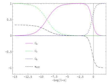
Figure 1: Plot of $\Omega_{m},\;\Omega_{r}$ (radiation density),$\;\Omega_{Vect}$ and the effective eq of state $w_{eff}$ as a function of the redshift $x=-Log[1+z]$ for $f=\lambda(\chi-\bar{\chi})$, and $U=\alpha\,(b^{2}-m_{b}^{2})^{2}$ with $\alpha=-2.8\,10^{-10},\,\bar{\chi}=5.5\,10^{-51}\,GeV^{2}$ and $m_{b}=10^{-10}\,GeV$.

Figure 2: Plot of $\Omega_{m},\;\Omega_{r},\;\Omega_{Vect}$ and $w_{eff}$ as a function of the redshift $x=-Log[1+z]$ for $f=\lambda(\chi-\bar{\chi})$, and $U=\alpha\,b^{4}$ with $\alpha=\,10^{-22},\,\bar{\chi}=8\,10^{-47}\,GeV^{2}$. In the internal square we plot also the ratio between the $z-$dependent Hubble parameter of our model over the $\Lambda$CDM scenario with the same late time $z=0$ values of $\Omega_{m}$ and $\Omega_{\Lambda}=\Omega_{Vect}$.

For the potential $U=\alpha\,(b^{2}-m_{b})^{2}$ we find at $x=0$ an effective eq of state $w_{eff}=-0.7$ with ${\cal A}=0.49$ and ${\cal R}=1.75$ and a time dependent Hubble expansion identical to the normal $\Lambda$CDM scenario having the same late time ($x=0$) values of $\Omega_{m}$ and $\Omega_{\Lambda}=\Omega_{Vect}$: $H_{\Lambda CDM}[z]=\sqrt{\Omega_{m}(1+z)^{3}+\Omega_{\Lambda}}$ (see fig. 1).

For $U=\alpha\,b^{4}$ we find at $x=0$ an effective eq of state $w_{eff}=-1.48$ with ${\cal A}=0.58$ and ${\cal R}=1.85$ with a pronounced deviation from the $\Lambda$CDM scenario in the present time (see fig 2), note also the strange dependence of the effective eq of state that jump to $\sim-1.5$ around $z\sim 0$ and then recalibrate to $\sim-1$ in late time period.

A detailed analysis of of cosmological pictures obtained with these models (attractor points, etc. )has to be work out.

As a final comment we note that the presented scenario doesn’t fit with the main hypothesis of the CC no-go Weinberg theorem weinb due to the fact that it requires all fields to be constant on the vacuum. We stress, in fact, that in order to have a non trivial dynamics we need $\chi=\nabla^{\alpha}b_{\alpha}\neq 0$ all times and this simple fact lend wings to the mechanism of CC cancellation here described. A similar feature is present also in the TMT gk .

Many open problems are still to be investigated, first of all the presence of “anomalous” contributions in the sources of the EH eqs that can generate phenomenological interesting dynamical deviations from EH. It follows the study of the inflationary mechanism and the dynamics of the linear perturbations than can deserve surprises due to the higher derivative structure of the theory.

Acknowledgments: I would like to thanks A. Dolgov for stimulating discussions.

Appendix:

Some notes about vector dynamics:

$$\tilde{T}^{(b)}_{\mu\nu}=\frac{\partial{\cal L}_{b}}{\partial g^{\mu\nu}}=\frac{1}{\chi}\left(-\hat{B}_{\mu\nu}(\chi f^{\prime})+\frac{g_{\mu\nu}}{2}\nabla^{\alpha}(b_{\alpha}\chi f^{\prime})\right)+U^{\prime}\,b_{\mu}b_{\nu}$$

where $\hat{B}_{\mu\nu}(F)\equiv\frac{1}{2}(b_{\mu}\nabla_{\nu}F+b_{\nu}\nabla_{\mu}F),\;f^{\prime}\equiv\frac{\partial f}{\partial\chi}$,

$\;U^{\prime}\equiv\frac{\partial U}{\partial b^{2}}$. We give also the trace of eq (12)

$$m_{Pl}^{2}\,R=T^{(m)}+2{\cal L}_{m}+2\,\chi\,f^{\prime}+3\,U^{\prime}b^{2}-3\,m_{Pl}^{2}\,\frac{\nabla^{2}\chi}{\chi}$$

that with the vectorial eqs of motion gives

$$\nabla_{\mu} \left(T^{(m)}\!\!+{\cal L}_{m}+\chi\,f^{\prime}-f+3\,U^{\prime}\,b^{2}-U-\right.$$ (31)

$$\left.3\,m_{Pl}^{2}\frac{\nabla^{2}\chi}{\chi}\right)=-2\,\chi\,U^{\prime}\,b_{\mu}$$

References

- (1)
- (2) S. Weinberg, Rev. Mod. Phys. 61 (1989) 1.
- (3) S. M. Carroll, W. H. Press and E. L. Turner, Ann. Rev. Astron. Astrophys. 30 (1992) 499. S. M. Carroll, Living Rev. Rel. 4 (2001) 1. P. J. E. Peebles and B. Ratra, Rev. Mod. Phys. 75 (2003) 559. T. Padmanabhan, Phys. Rept. 380 (2003) 235. U. Ellwanger, arXiv:hep-ph/0203252. S. Nobbenhuis, Found. Phys. 36 (2006) 613.
- (4) J. J. van der Bij and H. van Dam, Physica 116A (1982) 307. W. G. Unruh, Phys. Rev. D 40 (1989) 1048. Y. J. Ng and H. van Dam, J. Math. Phys. 32 (1991) 1337 and Phys. Rev. Lett. 65 (1990) 1972 and Int. J. Mod. Phys. D 10 (2001) 49. E. Alvarez, JHEP 0503 (2005) 002.
- (5) F. Wilczek, Phys. Rept. 104 (1984) 143. W. Buchmuller and N. Dragon, Phys. Lett. B 207 (1988) 292 and Phys. Lett. B 223, 313 (1989).
- (6) E. I. Guendelman and A. B. Kaganovich, Phys. Rev. D 53 (1996) 7020; Mod. Phys. Lett. A 12 (1997) 2421; Phys. Rev. D 55, 5970 (1997); Phys. Rev. D 57 (1998) 7200; Mod. Phys. Lett. A 13 (1998) 1583; Phys. Rev. D 56 (1997) 3548; Phys. Rev. D 60 (1999) 065004. E. I. Guendelman, Mod. Phys. Lett. A 14 (1999) 1043; Class. Quant. Grav. 17 (2000) 361; Mod. Phys. Lett. A 14 (1999) 1397; arXiv:gr-qc/9901067; arXiv:hep-th/0106085; Found. Phys. 31 (2001) 1019. A. B. Kaganovich, Phys. Rev. D 63 (2001) 025022. E. I. Guendelman and O. Katz, Class. Quant. Grav. 20 (2003) 1715.
- (7) F. Gronwald, U. Muench, A. Macias and F. W. Hehl, Phys. Rev. D 58 (1998) 084021. F. Wilczek, Phys. Rev. Lett. 80 (1998) 4851.
- (8) A.S.Eddington,The Mathematical Theory of Gravity, CUP 1924. S. Deser and G. W. Gibbons, Class. Quant. Grav. 15 (1998) L35. M. N. R. Wohlfarth, Class. Quant. Grav. 21 (2004) 1927 [Erratum-ibid. 21 (2004) 5297]. D. Comelli and A. Dolgov, JHEP 0411 (2004) 062. D. Comelli, Phys. Rev. D 72 (2005) 064018.
- (9) J. R. Bond, G. Efstathiou and M. Tegmark, Mon. Not. Roy. Astron. Soc. 291 (1997) L33. A. G. Riess et al., arXiv:astro-ph/0611572.