Error Estimation and Atomistic-Continuum Adaptivity
for the Quasicontinuum Approximation
of a Frenkel-Kontorova Model

Abstract.

We propose and analyze a goal-oriented a posteriori error estimator for the atomistic-continuum modeling error in the quasicontinuum method. Based on this error estimator, we develop an algorithm which adaptively determines the atomistic and continuum regions to compute a quantity of interest to within a given tolerance. We apply the algorithm to the computation of the structure of a crystallographic defect described by a Frenkel-Kontorova model and present the results of numerical experiments. The numerical results show that our method gives an efficient estimate of the error and a nearly optimal atomistic-continuum modeling strategy.

1. Introduction

The quasicontinuum (QC) method [22, 23, 24] has been successfully used to efficiently couple atomistic and continuum models for crystalline solids and offers the possibility of computing mesoscale or macroscale properties by a nearly minimal number of degrees of freedom. Accurate modeling requires that an atomistic model be used in regions with highly non-uniform deformations such as around dislocations, whereas a continuum model can be used in regions with nearly uniform deformations to reduce the number of degrees of freedom.

It is usually not known a priori which regions of some specimen undergo uniform deformations and which do not, so a posteriori error estimation is important for the design of efficient numerical approximations by the quasicontinuum method. Since the purpose of a computation is often to obtain the value of a (usually local) quantity of interest to a desired error tolerance rather than to obtain a solution to a desired error tolerance for a global norm, there has been great interest in the development of goal-oriented error estimators for many problems. They are based on duality techniques and have been developed and used to adaptively refine finite element approximations of continuum problems [1, 3] and to study and control modeling error [19].

In this paper, we extend this approach to develop an a posteriori error estimator for the quasicontinuum method which quantifies the atomistic-continuum modeling error for a goal function and allows for an adaptive decision about which regions can be accurately modeled as a continuum and which regions need to be modeled atomistically. Methods to determine the optimal mesh size within the continuum region will be studied in a forthcoming paper.

Crystallographic defects [5] provide a challenge to validate atomistic-continuum error estimators and adaptivity. No such error estimators and adaptive methods currently exist for fully three-dimensional crystals. As a step in this direction, we develop a rigorous theory for a simple one-dimensional atomistic model for a defect that is a modification of the Frenkel-Kontorova model [15]. We add next-nearest-neighbor harmonic interactions between the atoms to the nearest-neighbor harmonic interactions between the atoms in the classical Frenkel-Kontorova model.

A priori analyses for various quasicontinuum approximations have been given in [13, 14, 8, 4, 10, 9, 21, 12]. An a posteriori analysis for a slightly different one-dimensional quasicontinuum approximation is given in [20]. The development and application of a goal-oriented error estimator for mesh coarsening in a two-dimensional quasicontinuum method is reported in [18, 17].

Let us mention that the continuum model used in the QC method, which coincides with the model obtained by the classical thermodynamic limit, is by far not the only reasonable continuum model to use. A method to derive continuum models which approximate atomistic models up to an arbitrarily high order has been proposed in [2].

The paper is organized as follows. In Section 2, we give a general formulation of the one-dimensional quasicontinuum approximation [23] that includes not only two-body and three-body potentials, but also many body potentials such as the embedded atom potential [6, 7]. In Section 3, we describe our extension of the Frenkel-Kontorova model and its quasicontinuum approximation. In Section 4, we introduce the primal and dual problems for our model and formulate our approach to goal-oriented error estimation.

Next, in Section 5 we extend the approach in [16] to develop an error estimator for atomistic-continuum modeling. This first error estimator does not allow a decomposition among the atoms that can be used for atomistic-continuum adaptivity, so we propose and analyze a less accurate second error estimator that does allow such a decomposition.

Finally, in Section 6 we propose an adaptive atomistic-continuum modeling algorithm and show that it gives an efficient estimate of the modeling error and a nearly optimal atomistic-continuum modeling strategy for the computation of defect structure.

2. Quasicontinuum Approximation

The departure point for the QC approximation is the potential energy of the atomistic system. The potential energy that is utilized fully models the properties of the system. The local minima of the potential energy model the metastable states of the system, and the potential energy can be used in Newton’s equations of motion to model the dynamical behavior.

The QC method approximates the potential energy of the atomistic system in two steps. First, we develop a continuum potential energy that will be used in the adaptively determined continuum region, and we then show how to reduce the degrees of freedom in the continuum region.

2.1. The Atomistic System

We assume that the atomistic system has $2M$ atoms with deformation given by $\mathbf{y}^{a}=(y^{a}_{-M+1},\dots y^{a}_{M})\in{\mathbb{R}}^{2M}$. Without loss of generality, we assume that the atoms are ordered so that their positions satisfy $y^{a}_{i}<y^{a}_{i+1}$. Furthermore, we assume that the atomistic total potential energy, $\mathcal{E}^{a}(\mathbf{y}^{a}),$ can be written as a sum over potential energies associated with each atom, $\mathcal{E}^{a}_{i}(\mathbf{y}^{a}),$ so that

$$\mathcal{E}^{a}(\mathbf{y}^{a})=\sum_{i=-M+1}^{M}\mathcal{E}^{a}_{i}(\mathbf{y}^{a}).$$ (2.1)

This decomposition can be found for most empirical potentials, including embedded atom potential energies [6, 7]. For example, if the atomistic total potential energy $\mathcal{E}^{a}(\mathbf{y}^{a})$ is given by

$$\mathcal{E}^{a}(\mathbf{y}^{a})=\sum_{i<j}\psi(y^{a}_{j}-y^{a}_{i}),$$ (2.2)

where $\psi(r)$ is an empirical two-body potential energy, then we can obtain the decomposition (2.1) by taking

$$\mathcal{E}^{a}_{i}(\mathbf{y}^{a})=\frac{1}{2}\sum_{j\neq i}\psi(y^{a}_{j}-y^{a}_{i}).$$ (2.3)

We note that $\mathcal{E}^{a}_{i}(\mathbf{y}^{a})$ can also contain contributions from external forces, such as for the Frenkel-Kontorova model described in Section 3, and can thus depend on $i.$

2.2. The Atomistic-Continuum Energy

For any deformation $\mathbf{y}^{a}\in{\mathbb{R}}^{2M},$ we let $L^{i,i+1}\mathbf{y}^{a}\in{\mathbb{R}}^{\mathbb{Z}}$ denote the linear extrapolation of the atomistic positions $y^{a}_{i}$ and $y^{a}_{i+1}$ given by

$$(L^{i,i+1}\mathbf{y}^{a})_{k}=(k-i)y^{a}_{i+1}+(i+1-k)y^{a}_{i}\qquad\text{for }k=-\infty,\dots,\infty.$$ (2.4)

The continuum potential energy $\mathcal{E}^{c}_{i}(\mathbf{y}^{a})$ of atom $i$ is obtained from the average of the atomistic potential energy $\mathcal{E}^{a}_{i}$ evaluated at the extrapolations $L^{i-1,i}\mathbf{y}^{a}$ and $L^{i,i+1}\mathbf{y}^{a}$ by

$$\mathcal{E}^{c}_{i}(\mathbf{y}^{a}):={\textstyle\frac{1}{2}}\mathcal{E}^{a}_{i}(L^{i-1,i}\mathbf{y}^{a})+{\textstyle\frac{1}{2}}\mathcal{E}^{a}_{i}(L^{i,i+1}\mathbf{y}^{a}),$$ (2.5)

where we note that the domain of $\mathcal{E}^{a}_{i}$ has been expanded to the infinite periodic atomistic systems in the range of $L^{i-1,i}$ and $L^{i,i+1}.$ We assume that $\mathcal{E}^{a}_{i}$ is finite for infinite periodic atomistic systems, which is true for (2.3) when the two-body potential $\psi(r)$ decays fast enough so that $\sum_{k=1}^{\infty}\psi(kr)$ is finite for $r\neq 0.$ At the endpoints of the chain, the extrapolation can be done only to one side, so we neglect the undefined part and define

$$\mathcal{E}^{c}_{-M+1}(\mathbf{y}^{a}):={\textstyle\frac{1}{2}}\mathcal{E}^{a}_{-M+1}(L^{-M+1,-M+2}\mathbf{y}^{a})\qquad\text{and}\qquad\mathcal{E}^{c}_{M}(\mathbf{y}^{a}):={\textstyle\frac{1}{2}}\mathcal{E}^{a}_{M}(L^{M-1,M}\mathbf{y}^{a}).$$ (2.6)

We then decide for each atom $i$ whether to model its energy atomistically by $\mathcal{E}^{a}_{i}(\mathbf{y}^{a})$ or as a continuum by $\mathcal{E}^{c}_{i}(\mathbf{y}^{a})$. We thus obtain for the whole chain the atomistic-continuum energy

$$\begin{split}\mathcal{E}^{ac}(\mathbf{y}^{a}):=&\sum_{i=-M+1}^{M}\delta^{a}_{i}\mathcal{E}^{a}_{i}(\mathbf{y}^{a})+\sum_{i=-M+1}^{M}\delta^{c}_{i}\mathcal{E}^{c}_{i}(\mathbf{y}^{a})\\ =&\sum_{i=-M+1}^{M}\delta^{a}_{i}\mathcal{E}^{a}_{i}(\mathbf{y}^{a})+{\textstyle\frac{1}{2}}\sum_{i=-M+2}^{M}\delta^{c}_{i}\mathcal{E}^{a}_{i}(L^{i-1,i}\mathbf{y}^{a})+{\textstyle\frac{1}{2}}\sum_{i=-M+1}^{M-1}\delta^{c}_{i}\mathcal{E}^{a}_{i}(L^{i,i+1}\mathbf{y}^{a}),\end{split}$$ (2.7)

where

$$\delta_{i}^{a}=\begin{cases}1&\text{if atom $i$ is modeled atomistically,}\\ 0&\text{if atom $i$ is modeled as continuum,}\end{cases}\qquad\text{and}\qquad\delta_{i}^{c}=1-\delta_{i}^{a}.$$ (2.8)

This approximation allows for a slightly faster evaluation of the energy and its derivatives, especially if $\mathcal{E}^{a}_{i}$ is long-ranged. However, it reveals its full strength only after the quasicontinuum coarsening to be described next. We note that sometimes atomistic degrees of freedom and energies are referred to as nonlocal and continuum degrees of freedom and energies are referred to as local [23].

2.3. Repatoms: Reduction of Degrees of Freedom

The quasicontinuum method allows a reduction of the number of degrees of freedom in the continuum region. To this end, we choose so-called representative atoms, or more briefly called repatoms. The repatoms are a subset of the original atoms. The quasicontinuum approximation of the energy is defined completely in terms of the repatoms.

We choose the repatoms by defining indices $\ell_{j}$ for $j=-N+1,\ldots,N$ where

$$-M+1=\ell_{-N+1}<\cdots<\ell_{j}<\ell_{j+1}<\cdots<\ell_{N}=M.$$

The atoms at $y^{a}_{i}$ for $i=\ell_{-N+1},\ell_{-N+2},\ldots,\ell_{N}$ are repatoms, and all of the remaining atoms are non-repatoms. We have that

$$\nu_{j}=\ell_{j+1}-\ell_{j}$$ (2.9)

gives the number of atomistic intervals between the repatoms $\ell_{j}$ and $\ell_{j+1}.$ We require that the chain not be coarsened in the atomistic regions, which precisely means that $\delta^{c}_{\ell_{j}}=\delta^{c}_{\ell_{j}+1}=\ldots=\delta^{c}_{\ell_{j+1}}=1$ whenever $\nu_{j}>1$.

Finally, the interactions of the atomistic energy only partially reach into the continuum part if the atomistic potential has a finite cutoff radius. To allow for an exact calculation of this energy without atomistic interpolation, we require that these regions are not coarsened as well. As we will see in the next subsection, the atomistic next-nearest-neighbor interactions from the Frenkel-Kontorova model studied in this paper reach two atoms into the continuum part. Hence, we require that $\nu_{j-2}=\nu_{j-1}=\nu_{j}=\nu_{j+1}=1$ whenever $\delta^{a}_{\ell_{j}}=1$. Other potential energies in general require similar conditions that depend on their cut-off radius.

We denote the position of the $j$-th repatom by $y^{qc}_{j}=y^{a}_{\ell_{j}}$ and the vector of all repatoms by $\mathbf{y}^{qc}\in{\mathbb{R}}^{2N}$.

2.4. The Quasicontinuum Energy

Now we define the quasicontinuum energy. To this end, the missing non-repatoms are implicitly reconstructed. We will see later that this helps to set up the QC model, but needs not be done for the actual computation.

The reconstruction is done by a linear interpolation between the nearest repatom to the right and to the left. That is, the vector of all atomistic positions is computed from the vector $\mathbf{y}^{qc}$ of repatom positions by

$$I:{\mathbb{R}}^{2N}\to{\mathbb{R}}^{2M},\qquad(I\mathbf{y}^{qc})_{\ell_{j}+m}:=\frac{\nu_{j}-m}{\nu_{j}}y^{qc}_{j}+\frac{m}{\nu_{j}}y^{qc}_{j+1},\qquad m=0,\ldots,\nu_{j}.$$ (2.10)

We note that

$$y^{qc}_{j}=(I\mathbf{y}^{qc})_{\ell_{j}}.$$ (2.11)

The underlying idea is that in regions where the lattice spacing of the atoms is nearly constant, this interpolation is very close to the actual atomistic positions and therefore leads to a good approximation of the total energy. Only a few repatoms are needed in these regions. This exactly corresponds to mesh coarsening in classical finite element approximations of continuum models. On the other hand, in regions where the lattice spacing is non-uniform, such as around a dislocation, all atoms must be chosen to be repatoms to obtain sufficient accuracy. This guarantees that the full resolution of the atomistic model in the critical regions is retained and corresponds to a high refinement in classical finite element continuum models.

We define the QC approximation of the total energy to be

$$\mathcal{E}^{qc}(\mathbf{y}^{qc}):=\mathcal{E}^{ac}(I\mathbf{y}^{qc}).$$ (2.12)

Now (2.12) has to be reformulated such that it can be computed efficiently, without the overhead of the interpolation. Most atomistic potentials are invariant to translations, a property that allows us to simplify (2.12) considerably. For any translationally invariant energy $\mathcal{E}^{a}_{i}$, we have that $\mathcal{E}^{a}_{i}(L^{i,i+1}\mathbf{y}^{a})=\phi_{i}(y^{a}_{i+1}-y^{a}_{i})$ and $\mathcal{E}^{a}_{i}(L^{i-1,i}\mathbf{y}^{a})=\phi_{i}(y^{a}_{i}-y^{a}_{i-1})$ for some function $\phi_{i}$. If these functions $\phi_{i}$ coincide, that is, $\phi_{i}=\phi_{j}$ for all $i$ and $j,$ we can write

$$\mathcal{E}^{a}_{i}(L^{i-1,i}\mathbf{y}^{a})=\phi\left(y^{a}_{i}-y^{a}_{i-1}\right)\qquad\text{and}\qquad\mathcal{E}^{a}_{i}(L^{i,i+1}\mathbf{y}^{a})=\phi\left(y^{a}_{i+1}-y^{a}_{i}\right)$$ (2.13)

for some function $\phi:{\mathbb{R}}\to{\mathbb{R}}$. Here $\phi$ plays the role of a continuum energy density and is given for the two-body potential (2.2) by

$$\phi(r)=\sum_{k=1}^{\infty}\psi(kr).$$

Equations (2.7), (2.12), and (2.13) lead to

$$\mathcal{E}^{qc}(\mathbf{y}^{qc}) =\sum_{i=-M+1}^{M}\delta^{a}_{i}\mathcal{E}^{a}_{i}(I\mathbf{y}^{qc})+{\textstyle\frac{1}{2}}\sum_{i=-M+2}^{M}\delta^{c}_{i}\mathcal{E}^{a}_{i}(L^{i-1,i}I\mathbf{y}^{qc})+{\textstyle\frac{1}{2}}\sum_{i=-M+1}^{M-1}\delta^{c}_{i}\mathcal{E}^{a}_{i}(L^{i,i+1}I\mathbf{y}^{qc})$$

$$=\sum_{i=-M+1}^{M}\delta^{a}_{i}\mathcal{E}^{a}_{i}(I\mathbf{y}^{qc})+{\textstyle\frac{1}{2}}\sum_{i=-M+2}^{M}\delta^{c}_{i}\phi((I\mathbf{y}^{qc})_{i}-(I\mathbf{y}^{qc})_{i-1})$$ (2.14)

$$\qquad\qquad+{\textstyle\frac{1}{2}}\sum_{i=-M+1}^{M-1}\delta^{c}_{i}\phi((I\mathbf{y}^{qc})_{i+1}-(I\mathbf{y}^{qc})_{i}).$$

Because $I\mathbf{y}^{qc}$ is the linear interpolation between two repatoms $y^{qc}_{j}$ and $y^{qc}_{j+1},$ we have

$$(I\mathbf{y}^{qc})_{i+1}-(I\mathbf{y}^{qc})_{i}=\frac{y^{qc}_{j+1}-y^{qc}_{j}}{\nu_{j}},\qquad i=\ell_{j},\ldots,\ell_{j+1}-1.$$ (2.15)

Hence,

$$\mathcal{E}^{qc}(\mathbf{y}^{qc})=\sum_{i=-M+1}^{M}\delta^{a}_{i}\mathcal{E}^{a}_{i}(I\mathbf{y}^{qc})+\sum_{j=-N+1}^{N-1}\omega_{j}\phi\left(\frac{y^{qc}_{j+1}-y^{qc}_{j}}{\nu_{j}}\right)$$ (2.16)

with weight factors

$$\omega_{j}={\textstyle\frac{1}{2}}\nu_{j}\big{(}\delta^{c}_{\ell_{j}}+\delta^{c}_{\ell_{j+1}}\big{)}=\begin{cases}0&\text{if both }y^{qc}_{j}\text{ and }y^{qc}_{j+1}\text{ are atomistic},\\ {\textstyle\frac{1}{2}}&\text{if exactly one of }y^{qc}_{j}\text{ and }y^{qc}_{j+1}\text{ is continuum},\\ \nu_{j}&\text{if both }y^{qc}_{j}\text{ and }y^{qc}_{j+1}\text{ are continuum}.\\ \end{cases}$$ (2.17)

The first sum corresponds to the atomistic region which will be a small region and is thus computationally inexpensive. The second sum only involves at most $2N$ terms which is a considerable reduction when $N\ll M.$

Note that the second term in formula (2.16) coincides with an integral over the energy density $\phi$ as it occurs in finite element discretizations of classical continuum mechanical models. Hence the apparently unmotivated definitions (2.7) and (2.5) of the continuum energy here result in what is commonly understood as a continuum energy. The linear interpolation operator $I$ resembles the Cauchy-Born hypothesis.

3. Frenkel-Kontorova Model

Dislocations are lines in crystals which represent a defect in the lattice structure [15], see Figure 1. Typically, there is a core of small radius surrounding the dislocation line where the lattice structure is highly deformed, but the lattice structure is nearly uniform outside the core. A simple one-dimensional model for a defect such as a dislocation is given by the Frenkel-Kontorova model [15]. Here, the elastic energy is modeled by harmonic interactions between the atoms in the one-dimensional chain and the misfit energy of the slip plane is modeled by a periodic potential. A more accurate model of the same form is given by the Peierls-Nabarro model [11].

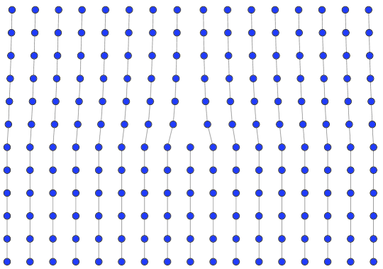
Figure 1. Cross-section through a dislocation in a three-dimensional cubic lattice. The displayed plane repeats periodically in the three-dimensional crystal. Vertical bonds are shown by lines to emphasize the topological defect.

3.1. Atomistic Frenkel-Kontorova Model

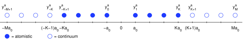
Figure 2. Numbering of the atoms. The dislocation is situated in the middle of the chain between atoms $y^{a}_{0}$ and $y^{a}_{1}$.

We study a single defect in the middle of the chain of $2M$ atoms. To achieve a symmetric description in terms of bonds, we number the atoms from $-M+1$ to $M$. The defect is situated between the atoms numbered 0 and 1 (Figure 2).

Recall that the atomistic positions are denoted by $\mathbf{y}^{a}=(y^{a}_{-M+1},\dots,y^{a}_{M})\in{\mathbb{R}}^{2M}$. The total potential energy for this atomistic system is then a function $\mathcal{E}^{a}:{\mathbb{R}}^{2M}\to{\mathbb{R}}$ of the atomistic positions. For the Frenkel-Kontorova model, the energy, $\mathcal{E}^{a}=\mathcal{E}^{a,e}+\mathcal{E}^{a,m}$, consists of two parts, namely the part which models the elastic energy of the defect, $\mathcal{E}^{a,e}$, and the part which models the misfit energy on the slip plane, $\mathcal{E}^{a,m}$.

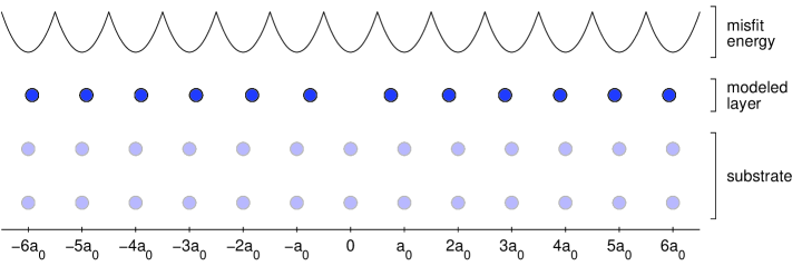
Figure 3. Frenkel-Kontorova model. The wells depict the misfit energy (3.4).

The elastic energy is modeled by Hookean (harmonic) springs between nearest-neighbors (NN) and next-nearest neighbors (NNN), and the total elastic energy is given by

$$\mathcal{E}^{a,e}(\mathbf{y}^{a})=\sum_{i=-M+1}^{M-1}{\textstyle\frac{1}{2}}k_{1}(y^{a}_{i+1}-y^{a}_{i}-a_{0})^{2}+\sum_{i=-M+2}^{M-1}{\textstyle\frac{1}{2}}k_{2}(y^{a}_{i+1}-y^{a}_{i-1}-2a_{0})^{2},$$ (3.1)

where the moduli $k_{1}>0$ and $k_{2}>0$ describe the strength of the elastic interactions, and where $a_{0}\in{\mathbb{R}}$ denotes the equilibrium distance.

We note that the asymptotic expansion to second order of any nonlinear NN/NNN potential energy

$$\mathcal{E}(\mathbf{y}^{a})=\sum_{i=-M+1}^{M-1}\psi(y^{a}_{i+1}-y^{a}_{i})+\sum_{i=-M+2}^{M-1}\psi(y^{a}_{i+1}-y^{a}_{i-1})$$ (3.2)

about $\mathbf{a}^{a}=\left[(-M+1)a_{0},(-M+2)a_{0},\cdots,(M-1)a_{0},Ma_{0}\right]^{T}\in{\mathbb{R}}^{2M}$ has the form

$$\begin{split}\mathcal{E}(\mathbf{y}^{a})&\approx\mathcal{E}(\mathbf{a}^{a})+\left(\psi^{\prime}(a_{0})+2\psi^{\prime}(2a_{0})\right)\sum_{i=-M+1}^{M-1}(y^{a}_{i+1}-y^{a}_{i}-a_{0})\\ &\qquad-\psi^{\prime}(2a_{0})(y^{a}_{M}-y^{a}_{M-1}-a_{0})-\psi^{\prime}(2a_{0})(y^{a}_{-M+2}-y^{a}_{-M+1}-a_{0})\\ &\qquad+{\textstyle\frac{1}{2}}\psi^{\prime\prime}(a_{0})\sum_{i=-M+1}^{M-1}(y^{a}_{i+1}-y^{a}_{i}-a_{0})^{2}+{\textstyle\frac{1}{2}}\psi^{\prime\prime}(2a_{0})\sum_{i=-M+2}^{M-1}(y^{a}_{i+1}-y^{a}_{i-1}-2a_{0})^{2}.\end{split}$$ (3.3)

We thus see that the elastic energy (3.1) with $k_{1}=\psi^{\prime\prime}(a_{0})$ and $k_{2}=\psi^{\prime\prime}(2a_{0})$ approximates the energy (3.2) to second order if $\psi^{\prime}(a_{0})+2\psi^{\prime}(2a_{0})=0$ and if we ignore the boundary terms in the second line of (3.3).

The misfit energy of the slip plane is modeled by a periodic potential (Figure 3). We model this misfit energy by

$$\mathcal{E}^{a,m}(\mathbf{y}^{a})=\sum_{i=-M+1}^{M}{\textstyle\frac{1}{2}}k_{0}\left(y^{a}_{i}-a_{0}\left\lfloor\frac{y^{a}_{i}}{a_{0}}+\frac{1}{2}\right\rfloor\right)^{2},$$ (3.4)

where $\lfloor x\rfloor$ denotes the largest integer smaller than or equal to $x$, and where the constant $k_{0}>0$ determines the strength of the misfit energy.

Altogether, the total potential energy of the atomistic system is given by

$$\begin{split}\mathcal{E}^{a}(\mathbf{y}^{a})&=\mathcal{E}^{a,e}(\mathbf{y}^{a})+\mathcal{E}^{a,m}(\mathbf{y}^{a})\\ &={\textstyle\frac{1}{2}}k_{1}\sum_{i=-M+1}^{M-1}(y^{a}_{i+1}-y^{a}_{i}-a_{0})^{2}+{\textstyle\frac{1}{2}}k_{2}\sum_{i=-M+2}^{M-1}(y^{a}_{i+1}-y^{a}_{i-1}-2a_{0})^{2}\\ &\qquad\qquad+{\textstyle\frac{1}{2}}k_{0}\sum_{i=-M+1}^{M}\left(y^{a}_{i}-a_{0}\left\lfloor\frac{y^{a}_{i}}{a_{0}}+\frac{1}{2}\right\rfloor\right)^{2}.\end{split}$$ (3.5)

We restrict ourselves to configurations in which the $M$ leftmost atoms $y_{i}^{a}$ for $-M+1\leq i\leq 0$ are situated in the interval $\left(\left(i-\frac{3}{2}\right)a_{0},\left(i-\frac{1}{2}\right)a_{0}\right)$, whereas the $M$ rightmost atoms $y_{i}^{a}$ for $1\leq i\leq M$ are situated in the interval $\left(\left(i-\frac{1}{2}\right)a_{0},\left(i+\frac{1}{2}\right)a_{0}\right)$. The defect is situated between atoms $y_{0}^{a}$ and $y_{1}^{a}.$ In this case, the total energy simplifies to

$$\begin{split}\mathcal{E}^{a}(\mathbf{y}^{a})&={\textstyle\frac{1}{2}}k_{1}\sum_{i=-M+1}^{M-1}(y^{a}_{i+1}-y^{a}_{i}-a_{0})^{2}+{\textstyle\frac{1}{2}}k_{2}\sum_{i=-M+2}^{M-1}(y^{a}_{i+1}-y^{a}_{i-1}-2a_{0})^{2}\\ &\qquad+{\textstyle\frac{1}{2}}k_{0}\sum_{i=-M+1}^{0}\left(y^{a}_{i}-(i-1)a_{0}\right)^{2}+{\textstyle\frac{1}{2}}k_{0}\sum_{i=1}^{M}\left(y^{a}_{i}-ia_{0}\right)^{2}.\end{split}$$ (3.6)

3.2. Quasicontinuum Approximation of the Frenkel-Kontorova Model

We now apply the quasicontinuum method to the dislocation model described in Section 3.1. The total energy (3.6) is split up into atom-wise contributions, separately for the elastic interactions and the misfit interactions:

$$\begin{split}\mathcal{E}^{a,e}_{i}(\mathbf{y}^{a})&={\textstyle\frac{1}{4}}k_{1}(y^{a}_{i}-y^{a}_{i-1}-a_{0})^{2}+{\textstyle\frac{1}{4}}k_{1}(y^{a}_{i+1}-y^{a}_{i}-a_{0})^{2}\\ &\quad+{\textstyle\frac{1}{4}}k_{2}(y^{a}_{i}-y^{a}_{i-2}-2a_{0})^{2}+{\textstyle\frac{1}{4}}k_{2}(y^{a}_{i+2}-y^{a}_{i}-2a_{0})^{2},\\ \mathcal{E}^{a,m}_{i}(\mathbf{y}^{a})&=\begin{cases}{\textstyle\frac{1}{2}}k_{0}\left(y^{a}_{i}-(i-1)a_{0}\right)^{2},&i=-M+1,\ldots,0,\\ {\textstyle\frac{1}{2}}k_{0}\left(y^{a}_{i}-ia_{0}\right)^{2},&i=1,\ldots,M.\end{cases}\end{split}$$ (3.7)

To simplify notation, we use the convention that the undefined terms at the endpoints of the chain are neglected. We thus have that

$$\mathcal{E}^{a}(\mathbf{y}^{a})=\mathcal{E}^{a,m}(\mathbf{y}^{a})+\mathcal{E}^{a,e}(\mathbf{y}^{a})=\sum_{i=-M+1}^{M}\left[\mathcal{E}^{a,m}_{i}(\mathbf{y}^{a})+\mathcal{E}^{a,e}_{i}(\mathbf{y}^{a})\right].$$ (3.8)

Since the largest displacement of the atoms is to be expected near the defect, we deem the atoms $-K+1,\ldots,K$ atomistic and the remaining atoms $-M+1,\ldots,-K$ and $K+1,\ldots,M$ continuum. Here $K<M$ is some constant whose optimal value will be determined by the algorithm given in Section 5.

The optimal choice of the repatoms for coarsening is investigated in the second paper of this series, so we work with a general formulation which holds for any values of $\ell_{j}$ for now. However, there are two restrictions on the coarsening. Since the atomistic region must not be coarsened and since we need full refinement in the vicinity of two atoms around the atomistic region due to the NNN interactions, we have that

$$\ell_{j}=j,\qquad j=-K-1,\ldots,K+2.$$ (3.9)

Second, we require that

$$\ell_{-N+1}=-M+1,\qquad\ell_{-N+2}=-M+2,\qquad\ell_{N-1}=M-1,\qquad\text{and}\qquad\ell_{N}=M$$ (3.10)

to incorporate the boundary conditions later.

The elastic part $\mathcal{E}^{a,e}_{i}$ is translationally invariant, so we perform its QC approximation as described in the previous section. This leads to the continuum energy density

$$\phi^{e}(r) ={\textstyle\frac{1}{2}}k_{1}(r-a_{0})^{2}+{\textstyle\frac{1}{2}}k_{2}(2r-2a_{0})^{2}$$

$$={\textstyle\frac{1}{2}}k_{12}(r-a_{0})^{2}$$ (3.11)

where $k_{12}:=k_{1}+4k_{2}.$

Regarding the misfit part $\mathcal{E}^{a,m}_{i}$, the above technique cannot be applied since the potential is not translationally invariant. However, there is a different summation technique to achieve a computationally efficient formulation which avoids the costly interpolation operator.

To shorten the notation, we let $\operatorname*{{\sum}^{\prime}}$ indicate the sum in which the first term and the last term are only counted half:

$$\operatorname*{{\sum}^{\prime}}_{i=m}^{n}x_{i}:={\textstyle\frac{1}{2}}x_{m}+\sum_{i=m+1}^{n-1}x_{i}+{\textstyle\frac{1}{2}}x_{n}$$ (3.12)

where $m<n$ and $x_{i}\in{\mathbb{R}}$. It is easy to verify that

$$\operatorname*{{\sum}^{\prime}}_{i=0}^{m}i^{2}=\frac{2m^{3}+m}{6}\qquad\text{and}\qquad\operatorname*{{\sum}^{\prime}}_{i=0}^{m}i(m-i)=\frac{m^{3}-m}{6}$$ (3.13)

for $m>0$.

For all pairs $(j,j+1)$ of continuum repatoms, we now reformulate all terms from (2.7) which involve the interaction between $\ell_{j}$ and $\ell_{j+1}$. For $j>0$, we get by definition (2.4) of the operator $L$, by definition (3.7) of $\mathcal{E}^{a,m}_{i}$, and by (3.13) that

$$\begin{split}{\textstyle\frac{1}{2}}\sum_{i=\ell_{j}+1}^{\ell_{j+1}}&\mathcal{E}^{a,m}_{i}(L^{i-1,i}I\mathbf{y}^{qc})+{\textstyle\frac{1}{2}}\sum_{i=\ell_{j}}^{\ell_{j+1}-1}\mathcal{E}^{a,m}_{i}(L^{i,i+1}I\mathbf{y}^{qc})\\ &={\textstyle\frac{1}{2}}\sum_{i=\ell_{j}+1}^{\ell_{j+1}}\mathcal{E}^{a,m}_{i}(I\mathbf{y}^{qc})+{\textstyle\frac{1}{2}}\sum_{i=\ell_{j}}^{\ell_{j+1}-1}\mathcal{E}^{a,m}_{i}(I\mathbf{y}^{qc})\\ &=\operatorname*{{\sum}^{\prime}}_{i=\ell_{j}}^{\ell_{j+1}}{\textstyle\frac{1}{2}}k_{0}\left(\frac{\ell_{j+1}-i}{\nu_{j}}y^{qc}_{j}+\frac{i-\ell_{j}}{\nu_{j}}y^{qc}_{j+1}-ia_{0}\right)^{2}\\ &=\operatorname*{{\sum}^{\prime}}_{i=\ell_{j}}^{\ell_{j+1}}{\textstyle\frac{1}{2}}k_{0}\left(\frac{\ell_{j+1}-i}{\nu_{j}}(y^{qc}_{j}-\ell_{j}a_{0})+\frac{i-\ell_{j}}{\nu_{j}}(y^{qc}_{j+1}-\ell_{j+1}a_{0})\right)^{2}\\ &={\textstyle\frac{1}{2}}k_{0}\frac{(y^{qc}_{j}-\ell_{j}a_{0})^{2}}{\nu_{j}^{2}}\operatorname*{{\sum}^{\prime}}_{i=\ell_{j}}^{\ell_{j+1}}(\ell_{j+1}-i)^{2}+{\textstyle\frac{1}{2}}k_{0}\frac{(y^{qc}_{j+1}-\ell_{j+1}a_{0})^{2}}{\nu_{j}^{2}}\operatorname*{{\sum}^{\prime}}_{i=\ell_{j}}^{\ell_{j+1}}(i-\ell_{j})^{2}\\ &\qquad+k_{0}\frac{(y^{qc}_{j}-\ell_{j}a_{0})(y^{qc}_{j+1}-\ell_{j+1}a_{0})}{\nu_{j}^{2}}\operatorname*{{\sum}^{\prime}}_{i=\ell_{j}}^{\ell_{j+1}}(\ell_{j+1}-i)(i-\ell_{j})\\ &={\textstyle\frac{1}{2}}k_{0}\frac{(y^{qc}_{j}-\ell_{j}a_{0})^{2}}{\nu_{j}^{2}}\frac{2\nu_{j}^{3}+\nu_{j}}{6}+{\textstyle\frac{1}{2}}k_{0}\frac{(y^{qc}_{j+1}-\ell_{j+1}a_{0})^{2}}{\nu_{j}^{2}}\frac{2\nu_{j}^{3}+\nu_{j}}{6}\\ &\qquad+k_{0}\frac{(y^{qc}_{j}-\ell_{j}a_{0})(y^{qc}_{j+1}-\ell_{j+1}a_{0})}{\nu_{j}^{2}}\frac{\nu_{j}^{3}-\nu_{j}}{6}\\ &=:\phi^{m}_{j+}(y^{qc}_{j},y^{qc}_{j+1}).\end{split}$$

For $j<0$, we similarly obtain

$$\begin{split}{\textstyle\frac{1}{2}}\sum_{i=\ell_{j}+1}^{\ell_{j+1}}&\mathcal{E}^{a,m}_{i}(L^{i-1,i}I\mathbf{y}^{qc})+{\textstyle\frac{1}{2}}\sum_{i=\ell_{j}}^{\ell_{j+1}-1}\mathcal{E}^{a,m}_{i}(L^{i,i+1}I\mathbf{y}^{qc})\\ &={\textstyle\frac{1}{2}}k_{0}\frac{(y^{qc}_{j}-(\ell_{j}-1)a_{0})^{2}}{\nu_{j}^{2}}\frac{2\nu_{j}^{3}+\nu_{j}}{6}+{\textstyle\frac{1}{2}}k_{0}\frac{(y^{qc}_{j+1}-(\ell_{j+1}-1)a_{0})^{2}}{\nu_{j}^{2}}\frac{2\nu_{j}^{3}+\nu_{j}}{6}\\ &\qquad+k_{0}\frac{(y^{qc}_{j}-(\ell_{j}-1)a_{0})(y^{qc}_{j+1}-(\ell_{j+1}-1)a_{0})}{\nu_{j}^{2}}\frac{\nu_{j}^{3}-\nu_{j}}{6}\\ &=:\phi^{m}_{j-}(y^{qc}_{j},y^{qc}_{j+1}).\end{split}$$

Since $\mathcal{E}^{a,m}_{-K}(L^{-K,-K+1}I\mathbf{y}^{qc})=\mathcal{E}^{a,m}_{-K}(I\mathbf{y}^{qc})$ and $\mathcal{E}^{a,m}_{K+1}(L^{K,K+1}I\mathbf{y}^{qc})=\mathcal{E}^{a,m}_{K+1}(I\mathbf{y}^{qc})$, the QC approximation of the chain can be given by

$$\begin{split}\mathcal{E}^{qc}(\mathbf{y}^{qc})=&\sum_{j=-N+1}^{-K}\left[w_{j}\phi^{e}\left(\frac{y^{qc}_{j+1}-y^{qc}_{j}}{\nu_{j}}\right)+\phi^{m}_{j-}(y^{qc}_{j},y^{qc}_{j+1})\right]\\ &+{\textstyle\frac{1}{2}}\mathcal{E}^{a,m}_{-K}(I\mathbf{y}^{qc})+\sum_{j=-K+1}^{K}\mathcal{E}^{a}_{i}(I\mathbf{y}^{qc})+{\textstyle\frac{1}{2}}\mathcal{E}^{a,m}_{K+1}(I\mathbf{y}^{qc})\\ &+\sum_{j=K}^{N-1}\left[w_{j}\phi^{e}\left(\frac{y^{qc}_{j+1}-y^{qc}_{j}}{\nu_{j}}\right)+\phi^{m}_{j+}(y^{qc}_{j},y^{qc}_{j+1})\right].\end{split}$$ (3.14)

Note that the interpolation $I\mathbf{y}^{qc}$ does not have to be computed here since the relevant terms only depend on uncoarsened parts of the chain.

Additionally, we will consider the atomistic-continuum approximation

$$\mathcal{E}^{ac}:{\mathbb{R}}^{2M}\to{\mathbb{R}}$$ (3.15)

of the atomistic energy without coarsening. It is given exactly like the QC approximation (3.14) with the only difference being that $\nu_{j}=1$ and $\ell_{j}=j$ everywhere.

4. Primal and Dual Problems

4.1. Problem Setup

We are now ready to set up the problems we will solve. We are interested in finding the minimum of the energy (3.14) subject to given boundary conditions.

We give the boundary conditions by constraining the deformation of two atoms at each end of the chain. This guarantees that the potential with next-nearest-neighbor interactions can be directly applied to all non-boundary atoms without having to neglect interactions. We define the spaces

$$V^{a}:={\mathbb{R}}^{2M},\qquad V^{a}_{0}:={\mathbb{R}}^{2M-4},\qquad V^{qc}:={\mathbb{R}}^{2N},\qquad V^{qc}_{0}:={\mathbb{R}}^{2N-4}.$$ (4.1)

The spaces $V^{a}$ and $V^{a}_{0}$ will also be used for the uncoarsened atomistic-continuum potential $\mathcal{E}^{ac}$, so there is no need to define spaces $V^{ac}$ and $V^{ac}_{0}$. We let ${\mathbf{y}}^{bc}\in V^{a}$ denote any vector which has the desired boundary values $y^{bc}_{-M+1},$ $y^{bc}_{-M+2},$ $y^{bc}_{M-1},$ and $y^{bc}_{M},$ and we let ${\mathbf{y}}^{bcq}\in V^{qc}$ by any vector satisfying (recall (3.10))

$$y^{bcq}_{-N+1} =y^{bc}_{-M+1}, y^{bcq}_{N-1} =y^{bc}_{M-1},$$

$$y^{bcq}_{-N+2} =y^{bc}_{-M+2}, y^{bcq}_{N} =y^{bc}_{M}.$$ (4.2)

For any vector $\mathbf{y}\in V^{a}_{0}$, we denote the extension by zero boundary conditions to be $J\mathbf{y}\in V^{a},$ so

$$J\mathbf{y}:=\begin{bmatrix}0&0&\mathbf{y}^{T}&0&0\end{bmatrix}^{T}\in{\mathbb{R}}^{2M},$$ (4.3)

and similarly we denote the extension by zero boundary conditions of $\mathbf{y}\in V^{qc}_{0}$ to be $J^{qc}\mathbf{y}\in V^{qc}$. The spaces of admissible solutions are then given by $JV^{a}_{0}+{\mathbf{y}}^{bc}\subset V^{a}$ and $J^{qc}V^{qc}_{0}+{\mathbf{y}}^{bcq}\subset V^{qc}$, respectively. We note that $J^{T}:V^{a}\to V^{a}_{0}$ is the restriction operator defined by

$$(J^{T}{\mathbf{y}})_{j}=y_{j}\quad\text{for }j=-M+3,\dots,M-2.$$

The minima $\bar{\mathbf{y}}^{a}$, $\bar{\mathbf{y}}^{ac},$ and $\bar{\mathbf{y}}^{qc}$ of the energy functionals $\mathcal{E}^{a}$, $\mathcal{E}^{ac},$ and $\mathcal{E}^{qc}$ given by (3.6), (3.15), and (3.14) subject to the above “clamped” boundary conditions are characterized as

$$\bar{\mathbf{y}}^{a} :=\operatorname*{arg\,min}_{\mathbf{y}\in{JV^{a}_{0}+\mathbf{y}}^{bc}}\mathcal{E}^{a}(\mathbf{y})\in V^{a},$$ (4.4)

$$\bar{\mathbf{y}}^{ac} :=\operatorname*{arg\,min}_{\mathbf{y}\in{JV^{a}_{0}+\mathbf{y}}^{bc}}\mathcal{E}^{ac}(\mathbf{y})\in V^{a},$$ (4.5)

$$\bar{\mathbf{y}}^{qc} :=\operatorname*{arg\,min}_{\mathbf{y}\in{J^{qc}V^{qc}_{0}+\mathbf{y}}^{bcq}}\mathcal{E}^{qc}(\mathbf{y})\in V^{qc}.$$ (4.6)

We note that the minima are uniquely determined because $\mathcal{E}^{a}$, $\mathcal{E}^{ac}$, and $\mathcal{E}^{qc}$ are strictly convex.

4.2. Matrix Formulation

For the subsequent discussion, it will be convenient to reformulate the total energies in matrix notation:

$$\mathcal{E}^{a}(\mathbf{y}) ={\textstyle\frac{1}{2}}(\mathbf{y}-\mathbf{a}^{a})^{T}D^{aT}E^{a}D^{a}(\mathbf{y}-\mathbf{a}^{a})+{\textstyle\frac{1}{2}}(\mathbf{y}-\mathbf{b}^{a})^{T}K^{a}(\mathbf{y}-\mathbf{b}^{a}),$$ (4.7a)

$$\mathcal{E}^{ac}(\mathbf{y}) ={\textstyle\frac{1}{2}}(\mathbf{y}-\mathbf{a}^{a})^{T}D^{aT}E^{ac}D^{a}(\mathbf{y}-\mathbf{a}^{a})+{\textstyle\frac{1}{2}}(\mathbf{y}-\mathbf{b}^{a})^{T}K^{a}(\mathbf{y}-\mathbf{b}^{a}),$$ (4.7b)

$$\mathcal{E}^{qc}(\mathbf{y}) ={\textstyle\frac{1}{2}}(\mathbf{y}-\mathbf{a}^{qc})^{T}D^{qcT}E^{qc}D^{qc}(\mathbf{y}-\mathbf{a}^{qc})+{\textstyle\frac{1}{2}}(\mathbf{y}-\mathbf{b}^{qc})^{T}K^{qc}(\mathbf{y}-\mathbf{b}^{qc}).$$ (4.7c)

The matrices $D^{a}\in{\mathbb{R}}^{(2M-1)\times 2M}$ and $D^{qc}\in{\mathbb{R}}^{(2N-1)\times 2N}$ compute the distance between two adjacent atomistic positions; the matrices $E^{a}\in{\mathbb{R}}^{(2M-1)\times(2M-1)}$, $E^{ac}\in{\mathbb{R}}^{(2M-1)\times(2M-1)}$, and $E^{qc}\in{\mathbb{R}}^{(2N-1)\times(2N-1)}$ contain the spring constants $k_{1}$, $k_{2}$, and $k_{12};$ and the matrices $K^{a}\in{\mathbb{R}}^{(2M-1)\times(2M-1)}$ and $K^{qc}\in{\mathbb{R}}^{(2N-1)\times(2N-1)}$ contain the misfit constant $k_{0}$. The vectors $\mathbf{a}^{a},\mathbf{b}^{a}\in{\mathbb{R}}^{2M}$ and $\mathbf{a}^{qc},\mathbf{b}^{qc}\in{\mathbb{R}}^{2N}$ are constants describing the minimum energy deformations for the elastic energy and misfit energy. The precise and lengthy definitions for all of these matrices and vectors are given in Appendix A.

If we decompose $\bar{\mathbf{y}}^{a}=J\mathbf{y}^{a}+{\mathbf{y}}^{bc}$ for $\mathbf{y}^{a}\in V_{0}^{a},$ then the minimization problem is given as

$$\mathbf{y}^{a} =\operatorname*{arg\,min}_{\mathbf{y}\in V_{0}^{a}}\mathcal{E}^{a}(J\mathbf{y}+{\mathbf{y}}^{bc})$$

$$=\operatorname*{arg\,min}_{\mathbf{y}\in V_{0}^{a}}\Big{[}{\textstyle\frac{1}{2}}\big{(}J\mathbf{y}+{\mathbf{y}}^{bc}-\mathbf{a}^{a}\big{)}^{T}D^{aT}E^{a}D^{a}\big{(}J\mathbf{y}+{\mathbf{y}}^{bc}-\mathbf{a}^{a}\big{)}$$

$$\qquad\qquad\qquad+{\textstyle\frac{1}{2}}\big{(}J\mathbf{y}+{\mathbf{y}}^{bc}-\mathbf{b}^{a}\big{)}^{T}K^{a}\big{(}J\mathbf{y}+{\mathbf{y}}^{bc}-\mathbf{b}^{a}\big{)}\Big{]}.$$ (4.8)

We also decompose $\bar{\mathbf{y}}^{ac}=J\mathbf{y}^{ac}+{\mathbf{y}}^{bc}$ and $\bar{\mathbf{y}}^{qc}=J^{qc}\mathbf{y}^{qc}+{\mathbf{y}}^{bcq}$ for $\mathbf{y}^{ac}\in V_{0}^{a}$ and $\mathbf{y}^{qc}\in V_{0}^{qc}$, and we then formulate similar minimization problems for $\mathbf{y}^{ac}$ and $\mathbf{y}^{qc}.$ Therefore, $\mathbf{y}^{a}$, $\mathbf{y}^{ac},$ and $\mathbf{y}^{qc}$ are determined by the linear systems

$$M^{a}\mathbf{y}^{a} =\mathbf{f}^{a},$$ (4.9a)

$$M^{ac}\mathbf{y}^{ac} =\mathbf{f}^{ac},$$ (4.9b)

$$M^{qc}\mathbf{y}^{qc} =\mathbf{f}^{qc},$$ (4.9c)

where

$$\begin{split}M^{a}&:=J^{T}(D^{aT}E^{a}D^{a}+K^{a})J,\\ M^{ac}&:=J^{T}(D^{aT}E^{ac}D^{a}+K^{a})J,\\ M^{qc}&:=J^{qcT}(D^{qcT}E^{qc}D^{qc}+K^{qc})J^{qc},\\ \mathbf{f}^{a}&:=-J^{T}D^{aT}E^{a}D^{a}({\mathbf{y}}^{bc}-\mathbf{a}^{a})-J^{T}K^{a}({\mathbf{y}}^{bc}-\mathbf{b}^{a}),\\ \mathbf{f}^{ac}&:=-J^{T}D^{aT}E^{ac}D^{a}({\mathbf{y}}^{bc}-\mathbf{a}^{a})-J^{T}K^{a}({\mathbf{y}}^{bc}-\mathbf{b}^{a}),\\ \mathbf{f}^{qc}&:=-J^{qcT}D^{qcT}E^{qc}D^{qc}({\mathbf{y}}^{bcq}-\mathbf{a}^{qc})-J^{qcT}K^{qc}({\mathbf{y}}^{bcq}-\mathbf{b}^{qc}).\end{split}$$ (4.10)

We note that the matrices $M^{a}$, $M^{ac},$ and $M^{qc}$ are positive definite, so the total energies admit a single global minimum and no other local minimum.

4.3. Goal-Oriented Error Estimation

To compare the approximate QC model to the original atomistic model, we have to analyze how much the solution $\mathbf{y}^{a}$ of the atomistic model deviates from the solution $\mathbf{y}^{qc}$ of the QC model. This deviation, which can be viewed as an approximation error, can be measured in different ways, for example as $\|\mathbf{y}^{a}-J^{T}IJ^{qc}\mathbf{y}^{qc}\|$ for some norm $\|\mathbf{\cdot}\|$. Here we follow a different approach, namely we measure the error of a quantity of interest denoted by $Q(\mathbf{y})$ for some function $Q:{\mathbb{R}}^{2M-4}\to{\mathbb{R}}$. Hence, we intend to estimate

$$Q(\mathbf{y}^{a})-Q(J^{T}IJ^{qc}\mathbf{y}^{qc}).$$ (4.11)

We will assume for simplicity that $Q$ is linear and thus has a representation $Q(\mathbf{y})=\mathbf{q}^{T}\mathbf{y}$ for some vector $\mathbf{q}\in V^{a}_{0}$.

For our application, a natural quantity of interest is the size of the dislocation, that is, the distance between the two atoms $y_{0}$ and $y_{1}$ to the left and right of the dislocation. This gives us

$$Q(\mathbf{y})=\mathbf{q}^{T}\mathbf{y}=y_{1}-y_{0}\qquad\text{with}\qquad\mathbf{q}=[0,\ldots,0,-1,1,0,\ldots,0]^{T}.$$ (4.12)

Two different sources of error arise during the QC approximation, namely the localization of the potential energy, that is, the passage from the atomistic to the continuum formulation on the one hand, and the coarsening in the continuum region by the restriction to the repatoms on the other hand. We denote these two errors by

$$\mathbf{e}:=\mathbf{y}^{a}-\mathbf{y}^{ac}\qquad\text{and}\qquad\mathbf{e}^{acqc}:=\mathbf{y}^{ac}-J^{T}IJ^{qc}\mathbf{y}^{qc}.$$ (4.13)

It makes sense to study these sources independently. Employing the linearity of $Q$, we have that

$$|Q(\mathbf{y}^{a})-Q(J^{T}IJ^{qc}\mathbf{y}^{qc})|=|Q(\mathbf{e})+Q(\mathbf{e}^{acqc})|\leq|Q(\mathbf{e})|+|Q(\mathbf{e}^{acqc})|.$$ (4.14)

The error term $|Q(\mathbf{e})|$ will be studied in Section 5, and the error term $|Q(\mathbf{e}^{acqc})|$ will be studied in the second part of this paper series.

4.4. Dual Problems

To facilitate the goal-oriented error analysis, we introduce the dual problems

$$M^{a}\mathbf{g}^{a} =\mathbf{q},$$ (4.15a)

$$M^{ac}\mathbf{g}^{ac} =\mathbf{q},$$ (4.15b)

$$M^{qc}\mathbf{g}^{qc} =J^{qcT}I^{T}J\mathbf{q},$$ (4.15c)

for $\mathbf{g}^{a},\mathbf{g}^{ac}\in{\mathbb{R}}^{2M-4},$ and $\mathbf{g}^{qc}\in{\mathbb{R}}^{2N-4}$. We note that the dual problems differ from the primal problems only by the right hand side since the matrices $M^{a}$, $M^{ac},$ and $M^{qc}$ are symmetric.

The solutions $\mathbf{g}^{a}$, $\mathbf{g}^{ac}$ and $\mathbf{g}^{qc}$ can be viewed as influence functions: They describe how the error at a specific point in the domain influences the error measured in terms of the goal function.

Analogously to the primal errors (4.13), we define the dual errors

$$\hat{\mathbf{e}}:=\mathbf{g}^{a}-\mathbf{g}^{ac}\qquad\text{and}\qquad\hat{\mathbf{e}}^{acqc}:=\mathbf{g}^{ac}-J^{T}IJ^{qc}\mathbf{g}^{qc}.$$ (4.16)

In addition, we will need the primal and dual residuals

$$R^{a}(\mathbf{y}) :=M^{a}\left(\mathbf{y}^{a}-\mathbf{y}\right)=\mathbf{f}^{a}-M^{a}\mathbf{y},$$

$$R^{ac}(\mathbf{y}) :=M^{ac}\left(\mathbf{y}^{ac}-\mathbf{y}\right)=\mathbf{f}^{ac}-M^{ac}\mathbf{y},$$

$$\hat{R}^{a}(\mathbf{g}) :=M^{a}\left(\mathbf{g}^{a}-\mathbf{g}\right)=\mathbf{q}-M^{a}\mathbf{g},$$

$$\hat{R}^{ac}(\mathbf{g}) :=M^{ac}\left(\mathbf{g}^{ac}-\mathbf{g}\right)=\mathbf{q}-M^{ac}\mathbf{g}.$$ (4.17)

5. Error Estimation for Atomistic vs. Continuum Modeling

In this section, we estimate the error $|Q(\mathbf{e})|$ arising from the approximation of an atomistic model by a continuum model. We consider $\mathbf{y}^{ac}$ and $\mathbf{g}^{ac}$ to be computable, although in practice we can only compute the coarsened approximations $\mathbf{y}^{qc}$ and $\mathbf{g}^{qc}.$

To this end, we adapt a technique introduced in [16] and [19] to estimate the modeling error for an elasticity model with rapidly oscillating coefficients and its homogenized version. We generalize this technique such that it allows for different right hand sides $\mathbf{f}^{a}$ and $\mathbf{f}^{ac}$ of the primal problem (4.9) instead of a common right hand side as it is used in the above-mentioned works.

We have

$$Q(\mathbf{y}^{a})-Q(\mathbf{y}^{ac}) =\mathbf{q}^{T}\mathbf{e}=\mathbf{g}^{aT}M^{a}\mathbf{e}=(\mathbf{g}^{acT}+\hat{\mathbf{e}})M^{a}\mathbf{e}$$

$$=\mathbf{g}^{acT}R^{a}(\mathbf{y}^{ac})+\hat{\mathbf{e}}^{T}M^{a}\mathbf{e}.$$ (5.1)

The term $\mathbf{g}^{acT}R^{a}(\mathbf{y}^{ac})$ can be computed, whereas $\hat{\mathbf{e}}^{T}M^{a}\mathbf{e}$ cannot because both $\mathbf{e}$ and $\hat{\mathbf{e}}$ are numerically unknown. Instead, we estimate $\hat{\mathbf{e}}^{T}M^{a}\mathbf{e}$ from above and from below by quantities that actually can be computed.

We will give two different error estimators $\eta_{1}$ and $\eta_{2}$. Before, we need to derive some auxiliary estimates to facilitate their development and analysis.

5.1. Auxiliary Estimates

We reformulate the difference $\mathbf{y}^{a}-\mathbf{y}^{ac}$ of the respective solutions in terms of a difference of the energy matrices. To this end, we define the perturbation matrix

$$P:={\mathcal{I}}-(E^{a})^{-1}E^{ac}$$ (5.2)

where ${\mathcal{I}}$ denotes the identity matrix. Note that $E_{a}P=E^{a}-E^{ac}$.

Lemma 5.1.

For any $\alpha,\beta\in{\mathbb{R}},$ we have that

$$M^{a}(\alpha\mathbf{e}+\beta\hat{\mathbf{e}})=-J^{T}D^{aT}E^{a}PD^{a}\big{[}\alpha(J\mathbf{y}^{ac}+\mathbf{y}^{bc}-\mathbf{a}^{a})+\beta J\mathbf{g}^{ac}\big{]}.$$ (5.3)

Proof.

We conclude from (4.9) that

$$M^{a}\mathbf{e} =M^{a}\mathbf{y}^{a}-M^{ac}\mathbf{y}^{ac}+\left(M^{ac}-M^{a}\right)\mathbf{y}^{ac}$$

$$=\mathbf{f}^{a}-\mathbf{f}^{ac}+\left(M^{ac}-M^{a}\right)\mathbf{y}^{ac},$$ (5.4)

and similarly since $M^{a}\mathbf{g}^{a}=M^{ac}\mathbf{g}^{ac}=\mathbf{q}$ that

$$M^{a}\hat{\mathbf{e}}=M^{a}(\mathbf{g}^{a}-\mathbf{g}^{ac})=(M^{ac}-M^{a})\mathbf{g}^{ac}.$$ (5.5)

Thus, it follows from (4.10) and (5.2) that

$$\begin{split}M^{a}(\alpha\mathbf{e}+\beta\hat{\mathbf{e}})&=\alpha\left[(M^{ac}-M^{a})\mathbf{y}^{ac}+\mathbf{f}^{a}-\mathbf{f}^{ac}\right]+\beta(M^{ac}-M^{a})\mathbf{g}^{ac}\\ &=J^{T}D^{aT}(E^{ac}-E^{a})D^{a}\big{[}\alpha(J\mathbf{y}^{ac}+\mathbf{y}^{bc}-\mathbf{a}^{a})+\beta J\mathbf{g}^{ac}\big{]}\\ &=-J^{T}D^{aT}E^{a}PD^{a}\big{[}\alpha(J\mathbf{y}^{ac}+\mathbf{y}^{bc}-\mathbf{a}^{a})+\beta J\mathbf{g}^{ac}\big{]}.\end{split}$$ (5.6)

We note that the $K^{a}$-related terms cancel here, because they coincide for the atomistic model and the continuum model. ∎

Lemma 5.2.

We have that

$$\|\alpha\mathbf{e}+\beta\hat{\mathbf{e}}\|_{M^{a}}\leq\big{\|}PD^{a}\big{[}\alpha(J\mathbf{y}^{ac}+\mathbf{y}^{bc}-\mathbf{a}^{a})+\beta J\mathbf{g}^{ac}\big{]}\big{\|}_{E^{a}}.$$ (5.7)

We note that the right hand side is numerically computable.

Proof.

To shorten the notation, we abbreviate $\mathbf{z}=\alpha(J\mathbf{y}^{ac}+\mathbf{y}^{bc}-\mathbf{a}^{a})+\beta J\mathbf{g}^{ac}$. By Lemma 5.1, we have

$$\begin{split}\|\alpha\mathbf{e}+\beta\hat{\mathbf{e}}\|_{M^{a}}&=\sup_{\mathbf{v}\in V^{a}_{0}\setminus\{0\}}\frac{\mathbf{v}^{T}M^{a}(\alpha\mathbf{e}+\beta\hat{\mathbf{e}})}{\|\mathbf{v}\|_{M^{a}}}\\ &=\sup_{\mathbf{v}\in V^{a}_{0}\setminus\{0\}}\frac{-\mathbf{v}^{T}J^{T}D^{aT}E^{a}PD^{a}\mathbf{z}}{\|\mathbf{v}\|_{M^{a}}}\\ &\leq\sup_{\mathbf{v}\in V^{a}_{0}\setminus\{0\}}\frac{\|D^{a}J\mathbf{v}\|_{E^{a}}\|PD^{a}\mathbf{z}\|_{E^{a}}}{\|D^{a}J\mathbf{v}\|_{E^{a}}}\\ &=\|PD^{a}\mathbf{z}\|_{E^{a}}.\end{split}$$ (5.8)

Here we have used that $\|D^{a}J\mathbf{v}\|_{E^{a}}\leq\|\mathbf{v}\|_{M^{a}}$ because the matrix $K^{a}$ in (4.10) is positive definite. ∎

5.2. First Error Estimator

We are now ready to derive the first error estimator, $\eta_{1}$. By the parallelogram identity, we have for all $\sigma\neq 0$ that

$$\begin{split}\hat{\mathbf{e}}^{T}M^{a}\mathbf{e}&=(\sigma^{-1}\hat{\mathbf{e}}^{T})M^{a}(\sigma\mathbf{e})\\ &=\textstyle\frac{1}{4}\|\sigma\mathbf{e}+\sigma^{-1}\hat{\mathbf{e}}\|_{M^{a}}^{2}-\frac{1}{4}\|\sigma\mathbf{e}-\sigma^{-1}\hat{\mathbf{e}}\|_{M^{a}}^{2}.\end{split}$$ (5.9)

In the following, we will determine computable constants $\eta_{\text{low}}^{+}$, $\eta_{\text{low}}^{-}$, $\eta_{\text{upp}}^{+}$ and $\eta_{\text{upp}}^{-}$ such that

$$\begin{split}\eta_{\text{low}}^{+}\leq\|\sigma\mathbf{e}+\sigma^{-1}\hat{\mathbf{e}}\|_{M^{a}}\leq\eta_{\text{upp}}^{+},\\ \eta_{\text{low}}^{-}\leq\|\sigma\mathbf{e}-\sigma^{-1}\hat{\mathbf{e}}\|_{M^{a}}\leq\eta_{\text{upp}}^{-}.\end{split}$$ (5.10)

From Lemma 5.2, we immediately get the upper estimates $\eta_{\text{upp}}^{+}$ and $\eta_{\text{upp}}^{-}$:

$$\begin{split}\eta_{\text{upp}}^{+}&:=\big{\|}PD^{a}\big{[}\sigma(J\mathbf{y}^{ac}+\mathbf{y}^{bc}-\mathbf{a}^{a})+\sigma^{-1}J\mathbf{g}^{ac}\big{]}\big{\|}_{E^{a}},\\ \eta_{\text{upp}}^{-}&:=\big{\|}PD^{a}\big{[}\sigma(J\mathbf{y}^{ac}+\mathbf{y}^{bc}-\mathbf{a}^{a})-\sigma^{-1}J\mathbf{g}^{ac}\big{]}\big{\|}_{E^{a}}.\end{split}$$ (5.11)

We note that $\eta_{\text{low}}^{+}$, $\eta_{\text{low}}^{-}$, $\eta_{\text{upp}}^{+}$ and $\eta_{\text{upp}}^{-}$ will depend on $\sigma$, but the estimates (5.10) will hold for any $\sigma\neq 0$. We will now choose $\sigma$ in such a way that the estimates are as sharp as possible, that is, such that $\eta_{\text{upp}}^{+}$ and $\eta_{\text{upp}}^{-}$ are smallest.

Lemma 5.3.

Both $\eta_{\text{upp}}^{+}$ and $\eta_{\text{upp}}^{-}$ given by (5.11) attain their minima for

$$\bar{\sigma}:=\sqrt{\frac{\|PD^{a}J\mathbf{g}^{ac}\|_{E^{a}}}{\|PD^{a}(J\mathbf{y}^{ac}+\mathbf{y}^{bc}-\mathbf{a}^{a})\|_{E^{a}}}}.$$ (5.12)

Proof.

We have that

$$(\eta_{\text{upp}}^{\pm})^{2} =\sigma^{2}\big{\|}PD^{a}(J\mathbf{y}^{ac}+\mathbf{y}^{bc}-\mathbf{a}^{a})\big{\|}_{E^{a}}^{2}\pm 2\mathbf{g}^{acT}J^{T}D^{aT}P^{T}E^{a}PD^{a}(J\mathbf{y}^{ac}+\mathbf{y}^{bc}-\mathbf{a}^{a})$$

$$\qquad+\sigma^{-2}\big{\|}PD^{a}J\mathbf{g}^{ac}\big{\|}_{E^{a}}^{2}.$$ (5.13)

Setting the first derivative of the mapping $\sigma\mapsto(\eta_{\text{upp}}^{\pm})^{2}$ to zero, we obtain the condition

$$2\bar{\sigma}\big{\|}PD^{a}(J\mathbf{y}^{ac}+\mathbf{y}^{bc}-\mathbf{a}^{a})\big{\|}_{E^{a}}^{2}-2\bar{\sigma}^{-3}\big{\|}PD^{a}J\mathbf{g}^{ac}\big{\|}_{E^{a}}^{2}=0$$ (5.14)

for critical points of $(\eta_{\text{upp}}^{\pm})^{2}$. This equation has the unique positive solution (5.12). Because $\lim_{|\sigma|\to\infty}\eta_{\text{upp}}^{\pm}=\lim_{\sigma\to 0}\eta_{\text{upp}}^{\pm}=\infty$, this point corresponds to a minimum. Hence the quantities $\eta_{\text{upp}}^{\pm}$ attain their minima at $\sigma=\bar{\sigma}$. ∎

Regarding the lower bounds $\eta_{\text{low}}^{+}$ and $\eta_{\text{low}}^{-}$, we have

$$\begin{split}\|\bar{\sigma}\mathbf{e}\pm\bar{\sigma}^{-1}\hat{\mathbf{e}}\|_{M^{a}}&=\sup_{\mathbf{v}\in V^{a}_{0}\setminus\{0\}}\frac{\mathbf{v}^{T}M^{a}(\bar{\sigma}\mathbf{e}\pm\bar{\sigma}^{-1}\hat{\mathbf{e}})}{\|\mathbf{v}\|_{M^{a}}}\\ &=\sup_{\mathbf{v}\in V^{a}_{0}\setminus\{0\}}\frac{\mathbf{v}^{T}(\bar{\sigma}R^{a}(\mathbf{y}^{ac})\pm\bar{\sigma}^{-1}\hat{R}^{a}(\mathbf{g}^{ac}))}{\|\mathbf{v}\|_{M^{a}}}\\ &\geq\frac{\mathbf{v}_{0}^{T}(\bar{\sigma}R^{a}(\mathbf{y}^{ac})\pm\bar{\sigma}^{-1}\hat{R}^{a}(\mathbf{g}^{ac}))}{\|\mathbf{v}_{0}\|_{M^{a}}}\end{split}$$ (5.15)

for any vector $\mathbf{v}_{0}\in V^{a}_{0}\setminus\{0\}$. Numerically, we have the two vectors $\mathbf{y}^{ac}$ and $\mathbf{g}^{ac}$ at our disposal, hence it makes sense to take a linear combination $\mathbf{v}_{0}=\mathbf{y}^{ac}+\theta^{\pm}\mathbf{g}^{ac}$. Here we follow the strategy of [19] and choose $\theta^{\pm}$ as the critical points of $\eta_{\text{low}}^{\pm}$.

Lemma 5.4.

Let

$$\mathbf{r}^{\pm}=\bar{\sigma}R^{a}(\mathbf{y}^{ac})\pm\bar{\sigma}^{-1}\hat{R}^{a}(\mathbf{g}^{ac}).$$ (5.16)

Then the lower bounds

$$\eta_{\text{low}}^{\pm}:=\frac{(\mathbf{y}^{ac}+\theta^{\pm}\mathbf{g}^{ac})^{T}\mathbf{r}^{\pm}}{\|\mathbf{y}^{ac}+\theta^{\pm}\mathbf{g}^{ac}\|_{M^{a}}}$$ (5.17)

have a unique critical point for

$$\bar{\theta}^{\pm}:=\frac{\mathbf{r}^{\pm T}\mathbf{y}^{ac}\;\mathbf{g}^{acT}M^{a}\mathbf{y}^{ac}-\mathbf{r}^{\pm T}\mathbf{g}^{ac}\;\|\mathbf{y}^{ac}\|_{M^{a}}^{2}}{\mathbf{r}^{\pm T}\mathbf{g}^{ac}\;\mathbf{g}^{acT}M^{a}\mathbf{y}^{ac}-\mathbf{r}^{\pm T}\mathbf{y}^{ac}\;\|\mathbf{g}^{ac}\|_{M^{a}}^{2}}.$$ (5.18)

Proof.

We have

$$\frac{\>\mathrm{d}}{\>\mathrm{d}\theta^{\pm}}\eta_{\text{low}}^{\pm}=\frac{\mathbf{r}^{\pm T}\mathbf{g}^{ac}\|\mathbf{y}^{ac}+\theta^{\pm}\mathbf{g}^{ac}\|_{M^{a}}-\mathbf{r}^{\pm T}(\mathbf{y}^{ac}+\theta^{\pm}\mathbf{g}^{ac})\frac{(\mathbf{y}^{ac}+\theta^{\pm}\mathbf{g}^{ac})^{T}M^{a}\mathbf{g}^{ac}}{\|\mathbf{y}^{ac}+\theta^{\pm}\mathbf{g}^{ac}\|_{M^{a}}}}{\|\mathbf{y}^{ac}+\theta^{\pm}\mathbf{g}^{ac}\|_{M^{a}}^{2}}.$$ (5.19)

Setting this expression to zero and solving for $\theta^{\pm}$ leads to the above condition. ∎

However, let us note that this critical point is not necessarily a maximum of $\eta_{\text{low}}^{\pm},$ which would be optimal for bound (5.10). Depending on the actual vectors $\mathbf{y}^{ac}$ and $\mathbf{g}^{ac}$, it can be shown that this critical point could be a minimum.

Now we have all necessary ingredients to construct the error estimator $\eta_{1}$. From (5) and (5.9), we get the computable estimate

$$\textstyle\mathbf{g}^{acT}R^{a}(\mathbf{y}^{ac})+\frac{1}{4}(\eta_{\text{low}}^{+})^{2}-\frac{1}{4}(\eta_{\text{upp}}^{-})^{2}\leq Q(\mathbf{y}^{a})-Q(\mathbf{y}^{ac})\leq\mathbf{g}^{acT}R^{a}(\mathbf{y}^{ac})+\frac{1}{4}(\eta_{\text{upp}}^{+})^{2}-\frac{1}{4}(\eta_{\text{low}}^{-})^{2}.$$ (5.20)

At first sight, this looks like we could get an estimate for $|Q(\mathbf{y}^{a})-Q(\mathbf{y}^{ac})|$ from both above and below. However, this is only true if both the left hand side and the right hand side have the same sign, which in general does not hold. But we get the following estimate.

Theorem 5.1.

We have that

$$\left|Q(\mathbf{y}^{a})-Q(\mathbf{y}^{ac})\right|\leq\eta_{1},$$ (5.21)

where the computable error estimator is defined as

$$\textstyle\eta_{1}:=\max\left(\left|\mathbf{g}^{acT}R^{a}(\mathbf{y}^{ac})+\frac{1}{4}(\eta_{\text{low}}^{+})^{2}-\frac{1}{4}(\eta_{\text{upp}}^{-})^{2}\right|,\left|\mathbf{g}^{acT}R^{a}(\mathbf{y}^{ac})+\frac{1}{4}(\eta_{\text{upp}}^{+})^{2}-\frac{1}{4}(\eta_{\text{low}}^{-})^{2}\right|\right).$$ (5.22)

We note that the computation of the $\eta_{upp}^{\pm}$ terms involves the solution of a linear system with matrix $E^{a}$ as its inverse appears in the operator $P$. The matrix $E^{a}$ is not diagonal, but has condition number ${\mathcal{O}}(1)$. So this is negligible compared to what would be necessary to solve the original atomistic problem which includes the operator $D^{aT}E^{a}D^{a}$ with condition number ${\mathcal{O}}(M^{2})$.

5.3. Second Error Estimator

There is no reasonable way to decompose the error estimator $\eta_{1}$ into a sum of element-wise or atom-wise contributions due to the $\eta_{low}^{\pm}$ terms. Therefore, we derive another error estimator $\eta_{2}$ which allows for such a decomposition, at the price of a less accurate estimate than $\eta_{1}$.

Theorem 5.2.

We have that

$$\left|Q(\mathbf{y}^{a})-Q(\mathbf{y}^{ac})\right|\leq\eta_{2}\leq\sum_{i=-M+3}^{M-2}\eta_{2,i}^{at}+\sum_{i=-M+1}^{M-1}\eta_{2,i}^{el}$$ (5.23)

where the computable global error estimator $\eta_{2}$ and the computable local error estimators, $\eta_{2,i}^{at}$ and $\eta_{2,i}^{el}$, associated with atoms and elements, respectively, are defined as

$$\eta_{2}$$

(5.24)

Proof.

From (5) and Lemma 5.2, we conclude that

$$\begin{split}\left|Q(\mathbf{y}^{a})-Q(\mathbf{y}^{ac})\right|&\leq\left|\mathbf{g}^{acT}R^{a}(\mathbf{y}^{ac})\right|+\left|\hat{\mathbf{e}}^{T}M^{a}\mathbf{e}\right|\\ &\leq\left|\mathbf{g}^{acT}R^{a}(\mathbf{y}^{ac})\right|+\|\hat{\mathbf{e}}\|_{M^{a}}\|\mathbf{e}\|_{M^{a}}\\ &\leq\left|\mathbf{g}^{acT}R^{a}(\mathbf{y}^{ac})\right|+\|PD^{a}(J\mathbf{y}^{ac}+\mathbf{y}^{bc}-\mathbf{a}^{a})\|_{E^{a}}\|PD^{a}J\mathbf{g}^{ac}\|_{E^{a}}\\ &=\eta_{2},\end{split}$$ (5.25)

which gives us the global estimate. For the decomposition into local contributions, we further estimate

$$\begin{split}\eta_{2}&=\left|\mathbf{g}^{acT}R^{a}(\mathbf{y}^{ac})\right|+\|PD^{a}(J\mathbf{y}^{ac}+\mathbf{y}^{bc}-\mathbf{a}^{a})\|_{E^{a}}\|PD^{a}J\mathbf{g}^{ac}\|_{E^{a}}\\ &\leq\left|\mathbf{g}^{acT}R^{a}(\mathbf{y}^{ac})\right|+{\textstyle\frac{1}{2}}\|PD^{a}(J\mathbf{y}^{ac}+\mathbf{y}^{bc}-\mathbf{a}^{a})\|_{E^{a}}^{2}+{\textstyle\frac{1}{2}}\|PD^{a}J\mathbf{g}^{ac}\|_{E^{a}}^{2}\\ &\leq\sum_{i=-M+3}^{M-2}\left|g^{ac}_{i}R^{a}(\mathbf{y}^{ac})_{i}\right|+{\textstyle\frac{1}{2}}\sum_{i=-M+1}^{M-1}\left|(PD^{a}J\mathbf{g}^{ac})_{i}\big{(}(E^{a}-E^{ac})D^{a}J\mathbf{g}^{ac}\big{)}_{i}\right|\\ &\qquad+{\textstyle\frac{1}{2}}\sum_{i=-M+1}^{M-1}\left|\big{(}PD^{a}(J\mathbf{y}^{ac}+\mathbf{y}^{bc}-\mathbf{a}^{a})\big{)}_{i}\big{(}(E^{a}-E^{ac})D^{a}(J\mathbf{y}^{ac}+\mathbf{y}^{bc}-\mathbf{a}^{a})\big{)}_{i}\right|\\ &=\sum_{i=-M+3}^{M-2}\eta_{2,i}^{at}+\sum_{i=-M+1}^{M-1}\eta_{2,i}^{el},\end{split}$$ (5.26)

which completes the proof. ∎

Let us remark that instead of the first inequality in (5.26), one can get an apparently better estimate

$$\begin{split}\@ADDCLASS{ltx_eqn_lefteqn}$\displaystyle\|PD^{a}(J\mathbf{y}^{ac}+\mathbf{y}^{bc}-\mathbf{a}^{a})\|_{E^{a}}\|PD^{a}J\mathbf{g}^{ac}\|_{E^{a}}$\mbox{}\hfil\\ &\qquad\qquad={\textstyle\frac{1}{2}}\gamma\|PD^{a}(J\mathbf{y}^{ac}+\mathbf{y}^{bc}-\mathbf{a}^{a})\|^{2}_{E^{a}}+{\textstyle\frac{1}{2}}\gamma^{-1}\|PD^{a}J\mathbf{g}^{ac}\|^{2}_{E^{a}}\end{split}$$ (5.27)

by introducing the additional weight factor

$$\gamma:=\frac{\|PD^{a}J\mathbf{g}^{ac}\|_{E^{a}}}{\|PD^{a}(J\mathbf{y}^{ac}+\mathbf{y}^{bc}-\mathbf{a}^{a})\|_{E^{a}}},$$ (5.28)

and then decomposing the resulting terms similar to the above. However, our numerical results showed that this modification does not significantly improve the decomposed error estimator for the application considered here.

6. Numerics

In the preceding sections, we constructed the error estimators $\eta_{1}$ and $\eta_{2}$. We will now give an algorithm for adaptive atomistic-continuum modeling based on these error estimators. Then we will present and discuss some numerical results.

6.1. Algorithm

The error estimator $\eta_{1}$ should give a better estimate of the error than $\eta_{2}$, because $\eta_{2}$ involves the inequality $\left|\hat{\mathbf{e}}^{T}M^{a}\mathbf{e}\right|\leq\|\hat{\mathbf{e}}\|_{M^{a}}\|\mathbf{e}\|_{M^{a}}$ in (5.25) in contrast to the parallelogram identity for $\eta_{1}$. However, $\eta_{2}$ can be decomposed into atom-wise and element-wise contributions $\eta_{2,i}^{at}$ and $\eta_{2,i}^{el}$, whereas the $\eta_{low}^{\pm}$ terms in $\eta_{1}$ do not admit a reasonable decomposition that can be used for atomistic-continuum adaptivity.

We make use of this by employing the sharper estimate $\eta_{1}$ to determine whether a given global error tolerance $\tau_{gl}$ for the error in an adaptive algorithm has already been achieved or not. If not, we use the decomposed estimates $\eta_{2,i}^{at}$ and $\eta_{2,i}^{el}$ to determine where the more precise atomistic modeling is needed. This leads us to the following algorithm:

1. Choose $\tau_{gl}$. Model all atoms as a continuum. Set $\tau_{at}\leftarrow\tau_{gl}$.

2. Solve primal problem (4.9b) for $\mathbf{y}^{ac}$ and dual problem (4.15b) for $\mathbf{g}^{ac}$.

3. Compute error estimator $\eta_{1}$ from (5.22).

4. If $\eta_{1}\leq\tau_{gl},$ then stop.

5. Compute local error estimators $\eta_{2,i}^{at}$ and $\eta_{2,i}^{el}$ from (5.24).

6. Set $\tau_{at}\leftarrow\frac{\tau_{at}}{\tau_{div}}$.

7. Make all atoms $i$ atomistic for which

   $$\eta_{2,i}^{tot}:=\eta_{2,i}^{at}+{\textstyle\frac{1}{2}}\big{(}\eta_{2,i-1}^{el}+\eta_{2,i}^{el}\big{)}\geq\tau_{at}.$$ (6.1)

8. Go to (2).

Here $\tau_{div}>1$ is a constant factor which describes how fast the atom-wise tolerance $\tau_{at}$ should decrease during adaption. Our experience has been that $\tau_{div}=10$ is a reasonable choice.

The crucial adaption step is (7). The adaption criterion (6.1) deems all atoms to be modeled atomistically if the associated error from the decomposition of $\eta_{2}$ exceeds the atomistic error tolerance $\tau_{at}$. Here the element-wise errors $\eta_{2,i}^{el}$ are distributed equally to the two adjacent atoms $i$ and $i+1$.

For the dislocation at the center of the chain and the chosen goal function, we expect that the atomistic repatoms always form a symmetric interval around the center. We have used the above adaptive atomistic-continuum algorithm to approximate our Frenkel-Kontorova model and have always found that the atomistic region is the set of atoms $-K+1,\ldots,K$ for some $K$ depending on $M$ and $\tau_{gl}.$ Thus, the modeling approach given in Section 3 of restricting to an atomistic region consisting of atoms $-K+1,\ldots,K$ for some $K$ rather than considering a more general atomistic region is justified a posteriori.

6.2. Numerical Results

The algorithm has been implemented as described above. The boundary conditions were chosen as

$$y^{bc}_{-M+1}=-M,\qquad y^{bc}_{-M+2}=-M+1,\qquad y^{bc}_{M-1}=M-1,\qquad y^{bc}_{M}=M.$$ (6.2)

The elastic constants are $k_{0}=1$ and $k_{1}=k_{2}=2$.

M	iteration	K	$\tau_{at}$	$\eta_{1}$
100	1	0	1.000000e-10	3.899207e-02
	2	28	1.000000e-11	5.915080e-10
	3	32	1.000000e-12	4.878532e-11
1000	1	0	1.000000e-10	3.899208e-02
	2	28	1.000000e-11	5.915100e-10
	3	32	1.000000e-12	4.878548e-11
10000	1	0	1.000000e-10	3.899208e-02
	2	28	1.000000e-11	5.915100e-10
	3	32	1.000000e-12	4.878548e-11
100000	1	0	1.000000e-10	3.899208e-02
	2	28	1.000000e-11	5.915099e-10
	3	32	1.000000e-12	4.878540e-11
1000000	1	0	1.000000e-10	3.899208e-02
	2	28	1.000000e-11	5.914422e-10
	3	32	1.000000e-12	4.871775e-11

Table 1. Convergence of the algorithm for $\tau_{gl}=10^{-10}$ and different values of $M$.

Table 1 shows how the algorithm given above performs. After 3 iterations, the desired accuracy $\tau_{gl}=10^{-10}$ is achieved. Moreover, we can see from the table that the number of iterations are independent of $M$, that means the algorithm behaves robustly with respect to the problem size $M$.

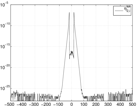
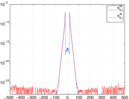
Figure 4. The error estimators $\eta_{2,i}^{tot}$ (left) and $\eta_{2,i}^{el},\eta_{2,i}^{at}$ (right) for $M=500$, $K=20$.

Figure 4 (left) shows the decomposition of the error estimator $\eta_{2}$ for a typical setting $M=500$, $K=20$. One can clearly see that the error in the atomistic region is small, whereas the error is large in the continuum regions that border the atomistic region. It then decreases exponentially towards the endpoints.

The error in both the atomistic region around the center and the continuum regions far away from the center are in the range of the (relative) machine precision $\varepsilon_{mach}$, which accounts for the fluctuations in these regions. The error can be considered to be numerically zero in these regions. In the continuum regions, we observe an error of magnitude ${\mathcal{O}}(\varepsilon_{mach}^{2})$, whereas in the continuum region we have ${\mathcal{O}}(\varepsilon_{mach})$, which leads to the different magnitudes of the fluctuations.

Figure 4 (right) shows the element-wise contributions $\eta_{2,i}^{el}$ and the atom-wise contributions $\eta_{2,i}^{at}$ of the decomposed error estimator $\eta_{2,i}^{tot}=\eta_{2,i}^{at}+{\textstyle\frac{1}{2}}\big{(}\eta_{2,i-1}^{el}+\eta_{2,i}^{el}\big{)}$. The atomistic part $\eta_{2,i}^{at}$, which corresponds to the $\mathbf{g}^{acT}R^{a}(\mathbf{y}^{ac})$ term, is dominant in the sense that it is about ten times larger than $\eta_{2,i}^{el}$, which comes from the estimate for the perturbation term $\hat{\mathbf{e}}^{T}M^{a}\mathbf{e}$. The fluctuations due to the limited machine precion in the atomistic region come from $\eta_{2,i}^{at}$, whereas those in the continuum region away from the defect stem from $\eta_{2,i}^{el}$. Let us note that in other applications of duality-based error estimation, the first term might not always be the dominant term. For example, in mesh refinement for classical linear finite elements, the first term even vanishes due to Galerkin orthogonality.

K	$|Q(\mathbf{y}^{a}-\mathbf{y}^{ac})|$	$\eta_{1}$	$\eta_{1}/|Q(\mathbf{y}^{a}-\mathbf{y}^{ac})|$	$\eta_{2}$	$\eta_{2}/|Q(\mathbf{y}^{a}-\mathbf{y}^{ac})|$
0	3.627633e-02	3.899208e-02	1.074863	3.999783e-02	1.102588
2	3.375762e-02	3.872272e-02	1.147081	5.101700e-02	1.511274
4	3.468605e-03	4.343595e-03	1.252260	5.422007e-03	1.563166
6	5.418585e-04	7.156249e-04	1.320686	9.187940e-04	1.695635
8	1.227067e-04	1.675383e-04	1.365356	2.193196e-04	1.787348
10	3.287188e-05	4.540984e-05	1.381419	5.984186e-05	1.820457
15	1.416914e-06	1.966114e-06	1.387603	2.597488e-06	1.833201
20	6.267636e-08	8.695824e-08	1.387417	1.148736e-07	1.832805
25	2.770161e-09	3.843388e-09	1.387424	5.077204e-09	1.832819
30	1.224369e-10	1.698739e-10	1.387440	2.244073e-10	1.832840
35	5.410783e-12	7.508365e-12	1.387667	9.918687e-12	1.833133
40	2.379208e-13	3.318024e-13	1.394592	4.383361e-13	1.842362
45	8.992806e-15	1.430733e-14	1.590975	1.901601e-14	2.114580
50	7.771561e-16	4.120094e-16	0.530150	6.201285e-16	0.797946

Table 2. Efficiency of the error estimators, $\eta_{1}/|Q(\mathbf{y}^{a}-\mathbf{y}^{ac})|$ and $\eta_{2}/|Q(\mathbf{y}^{a}-\mathbf{y}^{ac})|,$ for $M=1000$. For $K=45$ and $K=50$ the results become inaccurate due to limited machine precision.

Figure 5. Efficiency of the error estimators for $M=1000$.

Table 2 and Figure 5, which display the same data, show the efficiency of the error estimators, $\eta_{1}/|Q(\mathbf{y}^{a}-\mathbf{y}^{ac})|$ and $\eta_{2}/|Q(\mathbf{y}^{a}-\mathbf{y}^{ac})|,$ for $M=1000$. For comparison, the actual error is given as well. For the relatively small 1D problem, the actual error can be easily computed, whereas in real world applications it is of course not available. One can clearly see that $\eta_{1}$ gives a better estimate than $\eta_{2}$, which numerically confirms our conjecture that $\eta_{1}$ is a better estimator than $\eta_{2}$. We see that $\eta_{1}$ overestimates the actual error by a factor of 1.4, while $\eta_{2}$ is in a still acceptable range of 2 times the actual error. Moreover, we can see from Table 2 and Figure 5 that the error decreases exponentially with $K$.

$\tau_{gl}$	optimal $K$	$K$ by $\eta_{1}$	$K$ by $\eta_{2}$
1e-02	3	3	3
1e-03	5	5	5
1e-04	9	9	10
1e-05	12	13	13
1e-06	16	17	17
1e-07	20	20	21
1e-08	23	24	24
1e-09	27	28	28
1e-10	31	31	32
1e-11	35	35	35
1e-12	38	39	39
1e-13	42	42	43
1e-14	45	46	47

Table 3. Efficiency of the error estimators for $M=1000$.

Finally, we compare the optimal (smallest) value of $K$ which is needed to achieve a given accuracy $\tau_{gl}$ with the values for $K$ determined by the error estimators $\eta_{1}$ and $\eta_{2}$, again taking into account the precise error which is available for the model problem. We see from Table 3 that even $\eta_{2}$ only overestimates $K$ by at most 2 atoms. Thus, we get an efficient estimate of the required atomistic region for both error estimators.

Appendix A Matrix Definitions

We describe the matrices from Section 4.2. The matrix

$$D^{a}=\begin{bmatrix}-1&1\\ &-1&1\\ &&\ddots&\ddots\\ &&&-1&1\end{bmatrix}\in{\mathbb{R}}^{(2M-1)\times 2M}$$ (A.1)

transforms atomistic positions to distances between adjacent atoms. Similarly,

$$D^{qc}=\begin{bmatrix}-\nu_{-N+1}^{-1}&\nu_{-N+1}^{-1}\\ &-\nu_{-N+2}^{-1}&\nu_{-N+2}^{-1}\\ &&\ddots&\ddots\\ &&&-\nu_{N-1}^{-1}&\nu_{N-1}^{-1}\end{bmatrix}\in{\mathbb{R}}^{(2N-1)\times 2N}$$ (A.2)

transforms repatom positions from a coarsened chain to normalized distances between adjacent repatoms. The matrices

$$(E^{a})_{ij}=\begin{cases}k_{1}+k_{2}&i=j\in\{-M+1,M-1\}\\ k_{1}+2k_{2}&i=j\in\{-M+2,\ldots,M-2\}\\ k_{2}&|j-i|=1\\ 0&\text{otherwise},\end{cases}$$ (A.3)

$$(E^{ac})_{ij}=\begin{cases}{\textstyle\frac{1}{2}}k_{12}(\delta_{i}^{c}+\delta_{i+1}^{c})+{\textstyle\frac{1}{2}}k_{1}(\delta_{i}^{a}+\delta_{i+1}^{a})+{\textstyle\frac{1}{2}}k_{2}(\delta_{i-1}^{a}+\delta_{i}^{a}+\delta_{i+1}^{a}+\delta_{i+2}^{a})&i=j\\ {\textstyle\frac{1}{2}}k_{2}(\delta_{i}^{a}+\delta_{i+2}^{a})&j=i+1\\ {\textstyle\frac{1}{2}}k_{2}(\delta_{i-1}^{a}+\delta_{i+1}^{a})&j=i-1\\ 0&\text{otherwise},\end{cases}$$ (A.4)

and

$$(E^{qc})_{ij}=\begin{cases}\omega_{i}k_{12}+{\textstyle\frac{1}{2}}k_{1}(\delta_{i}^{a}+\delta_{i+1}^{a})+{\textstyle\frac{1}{2}}k_{2}(\delta_{i-1}^{a}+\delta_{i}^{a}+\delta_{i+1}^{a}+\delta_{i+2}^{a})&i=j\\ {\textstyle\frac{1}{2}}k_{2}(\delta_{i}^{a}+\delta_{i+2}^{a})&j=i+1\\ {\textstyle\frac{1}{2}}k_{2}(\delta_{i-1}^{a}+\delta_{i+1}^{a})&j=i-1\\ 0&\text{otherwise},\end{cases}$$ (A.5)

for $i,j=-M+1,\ldots,M-1$ and $i,j=-N+1,\ldots,N-1$, respectively, describe the spring interactions in terms of the distances between atoms or repatoms. Accordingly, the matrices

$$K^{a}=\begin{bmatrix}k_{0}\\ &\ddots\\ &&k_{0}\end{bmatrix}\in{\mathbb{R}}^{2M\times 2M}$$ (A.6)

and

$$(K^{qc})_{ij}=\begin{cases}\frac{1}{6}k_{0}\left[(2\nu_{i-1}+\nu_{i-1}^{-1})+(2\nu_{i}+\nu_{i}^{-1})\right]&i=j\in\{-N+2,\ldots,N-1\}\\ \frac{1}{6}k_{0}(2\nu_{-N+1}+\nu_{-N+1}^{-1})&i=j=-N+1\\ \frac{1}{6}k_{0}(2\nu_{N-1}+\nu_{N-1}^{-1})&i=j=N\\ \frac{1}{6}k_{0}(\nu_{i}-\nu_{i}^{-1})&j=i+1\\ \frac{1}{6}k_{0}(\nu_{j}-\nu_{j}^{-1})&j=i-1\\ 0&\text{otherwise},\end{cases}$$ (A.7)

for $i,j=-N+1,\ldots,N$ describe the misfit interactions for the original atomistic system and the QC approximation. Finally, the constant vectors

$$\mathbf{a}^{a}= \begin{bmatrix}(-M+1)a_{0}&(-M+2)a_{0}&\cdots&(M-1)a_{0}&Ma_{0}\end{bmatrix}^{T}\in{\mathbb{R}}^{2M},$$ (A.8a)

$$\mathbf{a}^{qc}= \begin{bmatrix}\ell_{-N+1}a_{0}&\ell_{-N+2}a_{0}&\cdots&\ell_{N-1}a_{0}&\ell_{N}a_{0}\end{bmatrix}^{T}\in{\mathbb{R}}^{2N},$$ (A.8b)

$$\mathbf{b}^{a}= \begin{bmatrix}-Ma_{0}&(-M+1)a_{0}&\cdots&-a_{0}&a_{0}&\cdots&(M-1)a_{0}&Ma_{0}\end{bmatrix}^{T}\in{\mathbb{R}}^{2M},$$ (A.8c)

$$\mathbf{b}^{qc}= \begin{bmatrix}(\ell_{-N+1}-1)a_{0}&(\ell_{-N+2}-1)a_{0}&\cdots&(\ell_{0}-1)a_{0}&\ell_{1}a_{0}&\cdots&\ell_{N-1}a_{0}&\ell_{N}a_{0}\end{bmatrix}^{T}\in{\mathbb{R}}^{2M},$$ (A.8d)

fix the equilibrium positions for the spring interactions and the misfit energy, respectively.

References

• [1] M. Ainsworth and J. T. Oden, A Posteriori Error Estimation in Finite Element Analysis, Wiley, New York, 2000.
• [2] M. Arndt and M. Griebel, Derivation of higher order gradient continuum models from atomistic models for crystalline solids, Multiscale Model. Simul., 4 (2005), pp. 531–562.
• [3] W. Bangerth and R. Rannacher, Adaptive Finite Element Methods for Differential Equations, Lectures in Mathematics, ETH Zürich, Birkhäuser, Basel, 2003.
• [4] X. Blanc, C. Le Bris, and F. Legoll, Analysis of a prototypical multiscale method coupling atomistic and continuum mechanics, Math. Model. Numer. Anal., 39 (2005), pp. 797–826.
• [5] P. M. Chaikin and T. C. Lubensky, Principles of Condensed Matter Physics, Cambridge University Press, 2000.
• [6] M. S. Daw and M. I. Baskes, Semiempirical, quantum mechanical calculation of hydrogen embrittlement in metals, Phys. Rev. Lett., 50 (1983), pp. 1285–1288.
• [7]  , Embedded-atom method: Derivation and application to impurities, surfaces, and other defects in metals, Phys. Rev. B, 29 (1984), pp. 6443–6453.
• [8] M. Dobson and M. Luskin, Analysis of a force-based quasicontinuum approximation, 2006, arXiv:math.NA/0611543.
• [9] W. E, J. Lu, and J. Z. Yang, Uniform accuracy of the quasicontinuum method, Phys. Rev. B, 74 (2006), p. 214115.
• [10] W. E and P. Ming, Analysis of multiscale methods, J. Comput. Math., 22 (2004), pp. 210–219.
• [11] E. Kaxiras, Atomic and Electronic Structure of Solids, Cambridge University Press, 2003.
• [12] J. Knap and M. Ortiz, An analysis of the quasicontinuum method, J. Mech. Phys. Solids, 49 (2001), pp. 1899–1923.
• [13] P. Lin, Theoretical and numerical analysis for the quasi-continuum approximation of a material particle model, Math. Comput., 72 (2003), pp. 657–675.
• [14]  , Convergence analysis of a quasi-continuum approximation for a two-dimensional material without defects, SIAM J. Numer. Anal., 45 (2007), pp. 313–332.
• [15] M. Marder, Condensed Matter Physics, John Wiley & Sons, 2000.
• [16] J. T. Oden and S. Prudhomme, Estimation of modeling error in computational mechanics, J. Comput. Phys., 182 (2002), pp. 496–515.
• [17] J. T. Oden, S. Prudhomme, and P. Bauman, Error control for molecular statics problems, Int. J. Multiscale Comput. Eng., 4 (2006), pp. 647–662.
• [18] J. T. Oden, S. Prudhomme, A. Romkes, and P. Bauman, Multiscale modeling of physical phenomena: Adaptive control of models, SIAM J. Sci. Comput., 28 (2006), pp. 2359–2389.
• [19] J. T. Oden and K. S. Vemaganti, Estimation of local modeling error and goal-oriented adaptive modeling of heterogeneous materials: Part I: Error estimates and adaptive algorithms, J. Comput. Phys., 164 (2000), pp. 22–47.
• [20] C. Ortner and E. Süli, A-posteriori analysis and adaptive algorithms for the quasicontinuum method in one dimension, Research Report NA-06/13, Oxford University Computing Laboratory, 2006.
• [21]  , A-priori analysis of the quasicontinuum method in one dimension, Research Report NA-06/12, Oxford University Computing Laboratory, 2006.
• [22] E. B. Tadmor, R. Miller, R. Phillips, and M. Ortiz, Nanoindentation and incipient plasticity, J. Mater. Res., 14 (1999), pp. 2233–2250.
• [23] E. B. Tadmor, M. Ortiz, and R. Phillips, Quasicontinuum analysis of defects in solids, Philos. Mag. A, 73 (1996), pp. 1529–1563.
• [24] E. B. Tadmor, R. Phillips, and M. Ortiz, Mixed atomistic and continuum models of deformation in solids, Langmuir, 12 (1996), pp. 4529–4534.