The Loewner driving function of trajectory arcs of quadratic differentials

Abstract.

We obtain a first order differential equation for the driving function of the chordal Loewner differential equation in the case where the domain is slit by a curve which is a trajectory arc of certain quadratic differentials. In particular this includes the case when the curve is a path on the square, triangle or hexagonal lattice in the upper half-plane or, indeed, in any domain with boundary on the lattice. We also demonstrate how we use this to calculate the driving function numerically. Equivalent results for other variants of the Loewner differential equation are also obtained: Multiple slits in the chordal Loewner differential equation and the radial Loewner differential equation. The proof of our theorem uses a generalization of Schwarz-Christoffel mapping to domains bounded by trajectory arcs of rotations of a given quadratic differential.

Introduction

Suppose that $\mathbb{H}=\{z\in\mathbb{C}:\mathrm{Im}(z)>0\}$ is the upper half-plane and $\gamma:[0,T)\mapsto\overline{\mathbb{H}}$ is a simple Jordan curve with $\gamma(0)\in\mathbb{R}$ and $\gamma(0,T)=\{\gamma(t):t\in(0,T)\}\subset\mathbb{H}$. Then for each $t\in(0,T)$,

$$H_{t}=\mathbb{H}\setminus\gamma(0,t]$$

is a simply-connected domain and hence by the Riemann mapping theorem, we can find a conformal map $f_{t}$ of $\mathbb{H}$ onto $H_{t}$. Moreover, we can require that $f_{t}$ has series expansion

$$f_{t}(z)=z-\frac{C(t)}{z}+O\left(\frac{1}{z^{2}}\right)\text{ as }z\rightarrow\infty.$$

Normalized in this way $f_{t}$ is unique and is said to be hydrodynamically normalized. The function $C(t)$ is positive, continuous and strictly increasing: it is called the half-plane capacity of $\gamma(0,t]$. Thus we can reparameterize $\gamma$ such that $C(t)=2t$ for all $t$, we will call this parameterization by half-plane capacity. With this normalization and parameterization, the function $f_{t}$ satisfies the differential equation (where $f_{t}^{\prime}$ denotes differentiation with respect to $z$ and $\dot{f}_{t}$ denotes differentiation with respect to $t$):

(0.1) $$\dot{f}_{t}(z)=-\frac{2f_{t}^{\prime}(z)}{z-\xi(t)},$$

where $\xi(t)=f_{t}^{-1}(\gamma(t))$ is a continuous real-valued function. This is the chordal Loewner differential equation; $\xi(t)$ is called the driving function of the slit $\gamma$. The converse is also true: given a measurable function $\xi$, the differential equation (0.1) with initial condition $f_{0}(z)\equiv z$ has solution $f_{t}$ which is a conformal map from $\mathbb{H}$ into itself (although $f(\mathbb{H})$ is not necessarily a slit domain). Chapter 3 and 4 of [7] gives full details of this construction.

Since Schramm’s discovery of stochastic Loewner evolution in 1999 (see [15]), there has been huge interest in the chordal Loewner differential equation and its variants. But the relationship between the slit in $\mathbb{H}$ and its resulting driving function is not well understood. There are a few papers that relate the behaviour of the slit with the behaviour of the driving function e.g. [10],[8]; also, the paper [2] calculates the slit arising from a few driving functions. In this paper, we will obtain a first order differential equation for $\xi$ (which we can then solve numerically) that allows us to calculate the driving function $\xi$ in the case where the curve $\gamma$ is a trajectory arc of a certain type of quadratic differential. We will show that this includes, for example, the case when $\gamma$ is a path on the square/triangle/hexagonal lattice in the upper half-plane or indeed, in any domain whose boundary lies on such a lattice. So for example, Figure 2 plots the driving function of a path on the hexagonal lattice in the upper half-plane and Figure 2 plots the driving function of a path on the square lattice in the upper half-plane.

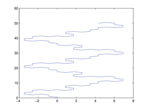
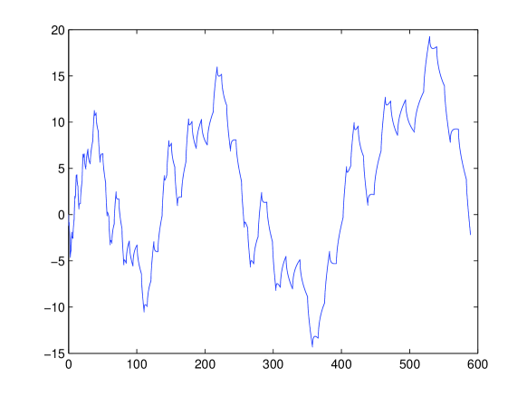
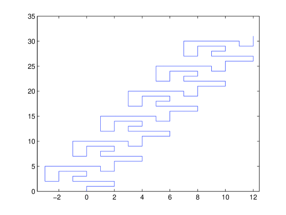
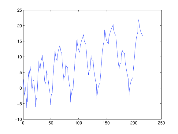
Figure 1. A path on the hexagonal lattice on the upper half-plane (left) and a plot of its driving function on the $y$-axis against time on the $x$-axis (right).

Figure 2. A path on the square lattice on the upper half-plane (left) and a plot of its driving function on the $y$-axis against time on the $x$-axis (right).

We also note that we can obtain equivalent results for other variants of the Loewner differential equation for example, in the radial version or with multiple slits. We will discuss this in the paper as well.

The proof of our formulae uses a generalization of Schwarz-Christoffel mapping to domains bounded by trajectory arcs of rotations of a given quadratic differential.

We also mention that, currently, the common method used to find the driving function of a given slit is to use the Zipper algorithm discovered independently by D. E. Marshall and R. Kühnau to approximate the function $f_{t}$ which can then be used to determine the driving function. The Zipper algorithm can be viewed as a discrete version of the Loewner differential equation and hence is well suited to studying growth processes. It also has the advantage of being very fast. See [11] and [3].

1. Main results

To state our main results, we have to provide some background in the theory of quadratic differentials. Note that not all the terms used here are standard in the literature. See Chapter 8 of [13] and [16] for more details. A quadratic differential on a domain $D\subset\widehat{\mathbb{C}}=\mathbb{C}\cup\{\infty\}$ is the formal expression

$$Q(z)dz^{2},$$

where $Q(z)$ is a meromorphic function on $D$. Then for $\omega\in D$ with $\omega\neq\infty$, $Q(z)$ has Laurent series expansion about $\omega$,

$$Q(z)=\sum_{k=n}^{\infty}a_{k}(z-\omega)^{k}$$

for some $n>-\infty$ with $a_{n}\neq 0$. Then we define the degree of $\omega$ with respect to $Q(z)dz^{2}$, $\deg_{Q}(\omega)$, to be equal to $n$.

If $\infty\in D$, then near $\infty$, $Q$ has Laurent series expansion given by

$$Q(z)=\sum_{k=m}^{\infty}b_{k}z^{-k},$$

then we define the degree of $\infty$ with respect to $Q(z)dz^{2}$, $\deg_{Q}(\infty)$ to be equal to $m-4$. The “4” in the definition ensures that the degree is conformally invariant in a way which we will make precise later. Then $\omega\in D$ is:

• a zero of $Q(z)dz^{2}$ if $\deg_{Q}(\omega)>0$.

• a pole of $Q(z)dz^{2}$ if $\deg_{Q}(\omega)<0$.

• an ordinary point of $Q(z)dz^{2}$ if $\deg_{Q}(\omega)=0$.

A trajectory arc of $Q(z)dz^{2}$ is a curve $\gamma:(a,b)\mapsto D$ that does not meet any zeroes and poles of $Q(z)dz^{2}$ and satisfies

$$Q(\gamma(t))\dot{\gamma}(t)^{2}>0\text{ for all }t\in(a,b).$$

For $\theta\in[0,\pi)$, a $\theta$-trajectory arc of $Q(z)dz^{2}$ is a curve $\gamma:(a,b)\mapsto D$ that satisfies

$$\arg[Q(\gamma(t))\dot{\gamma}(t)^{2}]=2\theta\text{ for all }t\in(a,b).$$

Then $\gamma$ is a $\theta$-trajectory arc of $Q(z)dz^{2}$ if and only if it is a trajectory arc of $e^{-2i\theta}Q(z)dz^{2}$. Hence, a $0$-trajectory arc is simply a trajectory arc and we call a $\pi/2$-trajectory arc an orthogonal trajectory arc. It is clear that these definitions are invariant under reparameterization of $\gamma$ so we will often call the point set of $\gamma$ a trajectory arc or $\theta$-trajectory arc. We call a maximal trajectory arc a trajectory and similarly, a maximal $\theta$-trajectory arc is called a $\theta$-trajectory. For example, if we consider the quadratic differential $1dz^{2}$ in $\mathbb{C}$, then the $\theta$-trajectories are the straight lines with gradient $\exp(2\theta)$.

We now consider a special type of quadratic differential: Let $D$ be a domain with piecewise analytic boundary. A Kühnau quadratic differential is a quadratic differential, $Q(z)dz^{2}$, on $D$ satisfying the following two properties:

Definition:

Let $D$ be a domain with piecewise analytic boundary. A Kühnau quadratic differential is a quadratic differential, $Q(z)dz^{2}$, on $D$ satisfying the following two properties:

1. We can write

   $$\partial D=\bigcup_{j=1}^{n}\overline{\Gamma}_{j}$$

   such that each $\Gamma_{j}$ is an open analytic arc with $\Gamma_{k}\cap\Gamma_{j}=\emptyset$ for $k\neq j$ and moreover, $Q(z)$ extends continuously to each $\Gamma_{j}$ and $\mathrm{arg}[Q(z)dz^{2}]$ is constant on each $\Gamma_{j}$ i.e. each $\Gamma_{j}$ is a $\theta_{j}$-trajectory arc for some $\theta_{j}\in[0,\pi)$.

2. At $z\in\overline{\Gamma}_{k}\cap\overline{\Gamma}_{j}$ for all $j\neq k$, there are either only finitely many direction from which trajectories approach the point $z$ or if there are infinitely many directions from which trajectories approach the point $z$, then for each such direction, there is only one trajectory that approaches $z$ at this direction.

These quadratic differentials are studied by Kühnau in [6] where he applies them to the study of certain Grötzsch-style extremal problems

Property (i) above, also implies that $D$ is locally connected. Thus each prime end of $D$ corresponds to a unique point in $\partial D$ (see [14, p. 27]). If, in addition, a point on $\partial D$ corresponds to a unique prime end, then we make no distinction between the two. Let $z$ be a prime end of $D$. Then we have 2 cases: Either $z\in\Gamma_{j}$ for some $j=1,\ldots,n$; or there exist exactly 2 of the $(\Gamma_{j})$, that end at the prime end $z$. In the latter case, we will denote $z$ by $z_{k}$ and assume that $\Gamma_{k}$, a $\theta_{k}$-trajectory arc, and $\Gamma_{k-1}$, a $\theta_{k-1}$-trajectory arc, are the only 2 arcs that end at $z_{k}$. Then we can define the degree of $z_{k}$ in $D$ with respect to $Q(z)dz^{2}$, $\mathrm{deg}_{D,Q}(z_{k})$, as follows:

$$\mathrm{deg}_{D,Q}(z_{k})=\left\{\begin{array}[]{ll}2[|\theta_{k}-\theta_{k-1}|/\pi+J_{k}-1]&\text{ if }\theta_{k}\neq\theta_{k-1},\\ 2J_{k}&\text{ if }\theta_{k}=\theta_{k-1},\end{array}\right.$$

where $J_{k}$ is the number of trajectories of $Q(z)dz^{2}$ inside $D$ that end at the prime end $z_{k}$. If $J_{k}$ is infinite, then the degree is not defined. Then for prime ends $z$ such that $z\in\Gamma_{j}$ for some $j=1,\ldots,n$, we define

$$\mathrm{deg}_{D,Q}(z)=0.$$

Although the motivation for this definition currently seems unclear, we will see that this indeed generalizes the concept of degree to points on the boundary. In particular, we will show that for $x\in\partial\mathbb{H}$, if $\mathrm{deg}_{\mathbb{H},Q}(x)\in\mathbb{Z}$, then $Q$ can be extended to a meromorphic function in a neighbourhood of $x$ with

$$\mathrm{deg}_{\mathbb{H},Q}(x)=\mathrm{deg}_{Q}(x).$$

We then have the following theorem on Kühnau quadratic differentials in $\mathbb{H}$:

Theorem 1.1.

Suppose that $Q(z)dz^{2}$ is a Kühnau quadratic differential on $\mathbb{H}$. Then we have

$$Q(z)=R\left(\prod_{j=1}^{n}(z-\zeta_{j})^{\lambda_{j}}\right)$$

for some constant $R\neq 0$, $\zeta_{j}\in\mathbb{C}$, $\lambda_{j}\in\mathbb{R}$ for $j=1,\ldots,n$.

This theorem can be viewed as a generalization of the Schwarz-Christoffel formula to domains bounded by $\theta_{k}$-trajectory arcs of a given quadratic differential.

We then have the following theorem on the Loewner driving function of a $\phi$-trajectory arc of a Kühnau quadratic differential $Q(z)dz^{2}$ that starts at a point $\xi_{0}\in\mathbb{R}$ with $\deg_{\mathbb{H},Q}(\xi_{0})=N\in\{0,1,\ldots\}$.

Theorem 1.2.

Suppose that $Q(z)dz^{2}$ is a Kühnau quadratic differential on $\mathbb{H}$ such that there is a point $\xi_{0}\in\mathbb{R}$ with $\deg_{\mathbb{H},Q}(\xi_{0})=N\in\{0,1,\ldots\}$; then we have

$$Q(w)=(w-\xi_{0})^{N}\left(\prod_{j=1}^{n}(w-a_{j})^{\alpha_{j}}\right),$$

where $a_{j}\in\mathbb{C}$ and $\alpha_{j}\in\mathbb{R}$. Let $\gamma:[0,T)\mapsto\partial{\mathbb{H}}$ be a simple curve such that $\gamma(0)=\xi_{0}$, $\gamma(0,T)\subset\mathbb{H}$ and $\gamma(0,T)$ is a $\phi$-trajectory arc of $Q(z)dz^{2}$ ($\phi\in[0,\pi)$) that is parameterized by half-plane capacity. Suppose that the functions $f_{t}$ maps $\mathbb{H}$ conformally onto $\mathbb{H}\setminus\gamma(0,t]$ and are hydrodynamically normalized. Then for $t\in(0,T)$

(1.1) $$2\xi(t)=-\mu^{-}C^{-}(t)-\mu^{+}C^{+}(t)-\left(\sum_{j=1}^{n}\alpha_{j}A_{j}(t)\right)+\Sigma_{0},$$

and

(1.2) $$\dot{\xi}(t)=-\frac{\mu^{-}}{C^{-}(t)-\xi(t)}-\frac{\mu^{+}}{C^{+}(t)-\xi(t)}-\left(\sum_{j=1}^{n}\frac{\alpha_{j}}{A_{j}(t)-\xi(t)}\right)$$

with initial condition $\xi(0)=\xi_{0}$. Where the functions $A_{j}(t)$ are defined by

$$A_{j}(t)=f_{t}^{-1}(a_{j})\text{ for }j=1,\ldots,n,$$

and $C^{+}(t)>C^{-}(t)$ are the two preimages of $\xi_{0}$ under $f_{t}$;

$$\mu^{\pm}=\mathrm{deg}_{\mathbb{H}\setminus\gamma(0,t],Q}(f_{t}(C^{\pm}(t))),$$

and

$$\Sigma_{0}=\left[N\xi_{0}+\left(\sum_{k=1}^{n}\alpha_{k}a_{k}\right)\right].$$

We can then use Theorem 1.2 to find the driving function in the case when the slit $\gamma$ consists of consecutive $\theta_{k}$-trajectory arcs of given quadratic differentials. We will explain how to do this in further detail later. One difficulty with using Theorem 1.2 is that the parameterization is inherently given in terms of half-plane capacity. This makes it difficult to calculate the driving function $\xi$ if we do not know anything about the half-plane capacity of the trajectory arc (which, in general, is the case). The next theorem will allow us to compare the parametrization with the length of the slit:

Theorem 1.3.

Suppose that $Q(z)dz^{2}$, $\gamma$ and $f_{t}$ are as defined in Theorem 1.2. Let

$$\Phi_{t}(z)=\frac{Q(f_{t}(z))f_{t}^{\prime}(z)^{2}}{(z-\xi(t))^{2}}.$$

Then $\gamma$ satisfies

(1.3) $$\dot{\gamma}(t)=-2\sqrt{\frac{\Phi_{t}(\xi(t))}{Q(\gamma(t))}}.$$

The rest of this paper is organized as follows: In the Section 2, we will state some basic results from the theory of quadratic differentials and use them to prove Theorem 1.1. Then we will use Theorem 1.1 to prove Theorems 1.2 and 1.3 in Section 3. In Section 4 we will discuss how to obtain the driving function numerically using Theorems 1.2 and 1.3. Finally in Section 5, we will discuss extensions of Theorem 1.2 to the case with multiple slits as well as to the radial Loewner differential equation.

2. Kühnau quadratic differentials and generalized Schwarz-Christoffel mapping

The aim of this section is to prove Theorem 1.1. We will first look at some of the basic results in the theory quadratic differentials that we will need.

Transformation Law

Suppose that $f$ is a conformal map from a domain $D_{2}$ onto a domain $D_{1}$ and suppose that $Q_{1}(w)dw^{2}$ is a quadratic differential on $D_{1}$. If we define

(2.1) $$Q_{2}(z)\equiv Q_{1}(f(z))f^{\prime}(z)^{2}$$

then $Q_{2}(z)dz^{2}$ is a quadratic differential on $D_{2}$. Then, it is clear that $\theta$-trajectory arcs are preserved by this transformation law i.e.

$$\gamma\text{ is a $\theta$-trajectory arc of }Q_{2}(z)dz^{2}\Leftrightarrow f\circ\gamma\text{ is a $\theta$-trajectory arc of }Q_{2}(w)dw^{2},$$

and also, for $z\in D_{2}$

$$\deg_{Q_{2}}(z)=\deg_{Q_{1}}(f(z)).$$

Hence trajectories and $\deg_{Q}$ are conformally invariant in the above sense.  

The following lemma tells us that the behaviour of a quadratic differential at a neighbourhood of a point is determined by the degree of that point.

Lemma 2.1 (Local behaviour of quadratic differentials).

Let $Q(z)dz^{2}$ be a quadratic differential on a domain $D$. Then for every $\omega\in D$ there is a conformal mapping $w=\phi(z)$ of some neighbourhood of $\omega$ such that

$$Q(z)dz^{2}=\left\{\begin{array}[]{ll}dw^{2}&\text{ if }\deg_{Q}(\omega)=0,\\ w^{n}dw^{2}&\text{ if }\deg_{Q}(\omega)=n\geq 1,\\ w^{-n}dw^{2}&\text{ if }\deg_{Q}(\omega)=-n\leq-1\text{ with $n$ odd},\\ c^{2}w^{-2}dw^{2}&\text{ if }\deg_{Q}(\omega)=-2,\\ (w^{-n}+cw^{-1})^{2}dw^{2}&\text{ if }\deg_{Q}(\omega)=-n\leq-4\text{ with $n$ even}.\end{array}\right.$$

Here, $c$ is the residue of a branch of $\sqrt{Q(z)}$ at $\omega$.

Proof.

See Theorem 8.1 of [13] or Section 6 of [16]. ∎

So since trajectories are conformally invariant this lemma tells us that the local structure of trajectories around a point $\omega\in D$ is completely determined by $\mathrm{deg}_{Q}(\omega)$ and the converse is true as well.

Lemma 2.2.

Suppose that $\omega\in D$ and $\deg_{Q}(\omega)=n$. Then

1. For $n\geq-1$, there are exactly $n+2$ trajectories of $Q(z)dz^{2}$ that end at $\omega$ and form equal angles with each other.

2. For $n\leq-3$, there are infinitely many trajectories ending at $\omega$ and moreover, there are $|n|-2$ directions at $\omega$ forming equal angles such that the trajectories approach $\omega$ in these directions.

3. For $n=-2$, the behaviour depends on the value of $c$ (as defined in Lemma 2.1).

   1. If $c$ is real, then the trajectories are the images of all radial lines under the map $\phi$ defined in Lemma 2.1.

   2. If $c$ is purely imaginary, then the trajectories are the images of all concentric circles under the map $\phi$ defined in Lemma 2.1.

   3. If $\mathrm{Re}[c],\mathrm{Im}[c]\neq 0$ then the trajectories are the images of logarithmic spirals under the map $\phi$ defined in Lemma 2.1.

Proof.

See Section 7 of [16]. ∎

This lemma shows that it makes sense for us to define $\deg_{D,Q}(x)$, the degree of a point on the boundary, in terms of the trajectories ending at $x$. If $D=\mathbb{H}$ and $Q$ extends to a meromorphic function on a neighbourhood of some $x\in\mathbb{R}\cup\{\infty\}$ with $\deg_{\mathbb{H},Q}(x)$ finite. Then by studying the trajectory structure at $x$, we can see that

$$\deg_{\mathbb{H},Q}(x)=\deg_{Q}(x).$$

This is the motivation for defining $\deg_{D,Q}$ in the way we have. The next lemma shows that the $\deg_{D,Q}$ is also conformally invariant:

Lemma 2.3.

Suppose that $Q(z)dz^{2}$ is a Kühnau quadratic differential on a domain $D$ and $f$ is a conformal map of the upper half-plane $\mathbb{H}$ onto $D$. Then the quadratic differential $Q_{f}(w)dw^{2}$ on $\mathbb{H}$, defined by $Q_{f}(w)=Q(f(w))f^{\prime}(w)^{2}$, is also a Kühnau quadratic differential. Moreover, suppose that $z\in\partial D$ is a prime end of $D$. Then

$$\deg_{D,Q}(z)=\deg_{\mathbb{H},Q_{f}}(f^{-1}(z)).$$

Proof.

By Carathéodory’s theorem, $f$ extends continuously to $\partial\mathbb{H}$ and by Schwarz’s reflection, $f$ extends analytically across $f^{-1}(\Gamma_{k})$ for all $k=1,\ldots,n$. Since $\theta$-trajectory arcs are conformally invariant, this implies that $Q_{f}$ defined by (2.1) is a Kühnau quadratic differential on $\mathbb{H}$. Moreover, for all $k=1,\ldots,n$, $f(\Gamma_{k})$ is a $\theta_{k}$-trajectory arc of $Q_{f}(z)dz^{2}$. Also each point on $\partial\mathbb{H}$ corresponds bijectively to a prime end of $\mathbb{H}$. Hence there is a bijective correspondence between the points of $\partial\mathbb{H}$ and prime ends of $D$. Then

$$\deg_{D,Q}(z)=\deg_{\mathbb{H},Q_{f}}(f^{-1}(z))$$

follows from the conformal invariance of trajectories. ∎

Reflection across trajectories

Suppose that $D$ is a domain such that $\Gamma\subset\partial D$ is an open interval in $\mathbb{R}$. Let $Q(z)dz^{2}$ be a quadratic differential such that $\Gamma$ is a trajectory arc or an orthogonal trajectory arc of $Q(z)dz^{2}$. Then let $D^{-}=\{\overline{z}:z\in D\}$ be the reflection of $D$ along $\Gamma$. Define

$$Q^{-}(z)=\overline{Q(\overline{z})}\text{ for }z\in D^{-}.$$

Then since $\Gamma$ is a trajectory, we have

$$Q(z)=Q^{-}(z)\in\mathbb{R}\text{ for }z\in\Gamma.$$

Thus by defining

(2.2) $$Q^{*}(z)=\left\{\begin{array}[]{ll}Q(z)&\text{ for }z\in D,\\ Q^{-}(z)&\text{ for }z\in D^{-},\\ Q(z)=Q^{-}(z)&\text{ for }z\in\Gamma.\end{array}\right.$$

it is easy to see that $Q^{*}$ is meromorphic in $D\cup D^{-}$ and hence $Q^{*}(z)dz^{2}$ is a quadratic differential on $D\cup D^{-}$. Thus by the transformation law (and using Schwarz reflection), this shows that we can extend quadratic differentials across trajectory arcs or orthogonal trajectory arcs.

We will use reflection to prove the following lemma:

Lemma 2.4.

Suppose $Q(z)dz^{2}$ is a Kühnau quadratic differential on $\mathbb{H}$. Then for any $z\in\partial\mathbb{H}$, $\deg_{\mathbb{H},Q}(z)\in\mathbb{Z}$ implies that $Q(z)dz^{2}$ extends to a quadratic differential on a neighbourhood of $z$ and hence

$$\deg_{\mathbb{H},Q}(z)=\deg_{Q}(z).$$

Proof.

Firstly, if $z\in\Gamma_{j}$ for some $j=1,\ldots,n$. Then by definition $\deg_{\mathbb{H},Q}(z)=0$ and $Q(z)dz^{2}$ can be extended to a neighbourhood of $z$ by reflection. By definition, every $z\in\Gamma_{j}$ is an ordinary point of $Q(z)dz^{2}$ and hence $\deg_{Q}(z)=\deg_{\mathbb{H},Q}(z)=0$.

Otherwise we write $z=z_{k}$ and suppose that a $\theta_{k-1}$-trajectory arc, $\Gamma_{k-1}$, and a $\theta_{k}$-trajectory arc, $\Gamma_{k}$, end at $z_{k}$. Then, by definition, $\deg_{\mathbb{H},Q}(z_{k})\in\mathbb{Z}$ implies that $\theta_{k}-\theta_{k-1}$ is a multiple of $\pi/2$. Thus $\Gamma_{k-1}$ and $\Gamma_{k}$ are trajectory arcs or orthogonal trajectory arcs of $e^{-2i\theta_{k-1}}Q(z)dz^{2}$. Thus by reflection, $e^{-2i\theta_{k-1}}Q(z)dz^{2}$ extends to a neighbourhood of $z_{k}$. Hence, $Q(z)dz^{2}$ also extends to a neighbourhood of $z_{k}$. ∎

We can now prove Theorem 1.1; but first, we explain briefly why we can view Theorem 1.1 as a generalized form of Schwarz-Christoffel mapping: Schwarz-Christoffel mapping is a method of computing the conformal map between the upper half-plane and a domain bounded by a polygon. See [12] for more details. If we have a conformal map $f$ from $\mathbb{H}$ to some domain $D$ such that the sides of $D$ consist of $\theta$-trajectory arcs of the quadratic differential $Q(w)dw^{2}$. Then $Q(w)dw^{2}$ is a Kühnau quadratic differential on $D$ and hence by Lemma 2.3, $Q(f(z))f^{\prime}(z)dz^{2}$ is a Kühnau quadratic differential on $\mathbb{H}$. Theorem 1.1 then implies that

$$Q(f(z))f^{\prime}(z)^{2}=R\left(\prod_{j=1}^{n}(z-\zeta_{j})^{\lambda_{j}}\right).$$

This is precisely the Schwarz-Christoffel formula when $Q(z)\equiv 1$.

Also, we comment that the case when $Q(w)dw^{2}$ is either negative or positive on $\mathbb{R}$ (i.e. the boundary of $\mathbb{R}$ consists only of trajectory arcs and orthogonal trajectory arcs) is easy to prove: we can use reflection to extend $Q(z)dz^{2}$ to a quadratic differential on the Riemann sphere $\widehat{\mathbb{C}}$. Hence $Q(z)$ must be rational since property (ii) in the definition of Kühnau quadratic differentials guarantees that $Q(z)$ does not have any essential singularities and so $Q(z)$ is rational (since the only meromorphic functions on $\widehat{\mathbb{C}}$ are rational). This proves Theorem 1.1 for this case.

Proof of Theorem 1.1.

Since $Q(z)dz^{2}$ is a Kühnau quadratic differential, we can find

$$z_{1}<\ldots<z_{m},$$

and

$$\Gamma_{k}=\left\{\begin{array}[]{l}(z_{k-1},z_{k})\text{ for }k=1,\ldots,m,\\ (z_{m},\infty)\text{ for }k=m+1,\\ (-\infty,z_{0})\text{ for }k=0,\end{array}\right.$$

such that each $\Gamma_{k}$ is a $\theta_{k}$-trajectory arc of $Q(z)dz^{2}$ for some $\theta_{k}\in[0,\pi)$. Let

$$\mathcal{T}=\left\{\Gamma_{1},\ldots,\Gamma_{m+1}\right\}.$$

Then take any $\Gamma\in\mathcal{T}$. Since $\Gamma$ is a $\theta$-trajectory for some $\theta$, $\Gamma$ is a trajectory arc of $e^{-2i\theta}Q(z)dz^{2}$; hence by reflection, we can reflect the quadratic differential $e^{-2i\theta}Q(z)dz^{2}$ across $\Gamma$ to get a quadratic differential on $\mathbb{H}^{-}=\{\mathrm{Im}(z)<0\}$ which we call $\widetilde{Q}(z)dz^{2}$. Similarly, by rotating $\widetilde{Q}(z)dz^{2}$, we can reflect it across another $\Upsilon\in\mathcal{T}$ to get another quadratic differential $Q^{*}(z)dz^{2}$ on $\mathbb{H}$. Since $Q^{*}$ is obtained from $Q$ by rotating twice, we have

$$Q^{*}(z)=e^{i\sigma}Q(z)$$

for some $\sigma\in[0,2\pi)$. This shows that

$$\Psi(z)=\frac{Q^{\prime}(z)}{Q(z)}=\frac{(Q^{*})^{\prime}(z)}{Q^{*}(z)}$$

can be extended to a meromorphic function in $\mathbb{C}\setminus\{z_{1},\ldots,z_{m}\}$. Then part (ii) of the definition of Kühnau quadratic differentials implies that all the finite singularities of $\Psi(z)$ are simple poles otherwise $Q(z)$ would have an essential singularity which, by the great Picard theorem, contradicts part (ii) of the definition of Kühnau quadratic differentials. Thus we can write:

$$\Psi(z)=h(z)-\left(\sum_{j=1}^{n}\frac{\lambda_{j}}{z-\zeta_{j}}\right),$$

where $\zeta_{j}\in\mathbb{C}$, and $\lambda_{j}\in\mathbb{R}$, and $h(z)$ is an entire function in $\mathbb{C}$ that does not does not vanish in $\mathbb{C}$. This implies that

$$Q(z)=\exp\left[\int^{z}h(\zeta)d\zeta\right]\left(\prod_{j=1}^{n}(z-\zeta_{j})^{\lambda_{j}}\right)\left(\prod_{k=1}^{m}(z-z_{k})^{\nu_{k}}\right).$$

Moreover, the singularity at $\infty$ of

$$\exp\left[\int^{z}h(\zeta)d\zeta\right]$$

cannot be essential by part (ii) of the definition of Kühnau quadratic differentials (otherwise we would get a contradiction with the great Picard theorem as above). This implies that

$$\exp\left[\int^{z}h(\zeta)d\zeta\right]$$

is constant (since it has no zeroes or poles). Hence

$$Q(z)=R\left(\prod_{j=1}^{n}(z-\zeta_{j})^{\lambda_{j}}\right).$$

∎

If $\zeta_{j}\in\mathbb{C}\setminus\mathbb{R}$, then by definition, we must have

$$\lambda_{j}=\deg_{Q}(\zeta_{j}).$$

Moreover, if $\zeta_{j}\in\mathbb{R}$ and $\deg_{\mathbb{H},Q}(\zeta_{j})<\infty$ we also have

$$\nu_{k}=\deg_{\mathbb{H},Q}(z_{k}).$$

We will not prove this fact here but in the following corollary we will consider a special case. The general proof follows readily from it. We will prove the following corollary which is simply an application of Theorem 1.1 to domains slit by $\phi$-trajectory arcs:

Corollary 2.5.

Suppose that $Q(z)dz^{2}$ is a Kühnau quadratic differential on $\mathbb{H}$ such that there is a point $\xi_{0}\in\mathbb{R}$ with $\deg_{\mathbb{H},Q}(\xi_{0})=N\in\{0,1,\ldots\}$; then we can write

(2.3) $$Q(w)=R(w-\xi_{0})^{N}\left(\prod_{j=1}^{n}(w-a_{j})^{\alpha_{j}}\right),$$

where $a_{j}\in\mathbb{C}$, $\alpha_{j}\in\mathbb{R}$, and also $R$ is some non-zero constant. Let $\gamma:[0,T]\mapsto\overline{\mathbb{H}}$ be a simple curve such that $\gamma(0)=\xi_{0}$ and $\gamma(0,T)$ is a $\phi$-trajectory arc of $Q(w)dw^{2}$ in $\mathbb{H}$ ($\phi\in[0,\pi)$) and $\zeta=\gamma(T)\in\mathbb{H}$ is an ordinary point of $Q(w)dw^{2}$ (i.e. $\deg_{Q}(\zeta)=0$). Suppose that $f$ maps $\mathbb{H}$ conformally onto $\mathbb{H}\setminus\gamma(0,T]$. Then $f$ satisfies

(2.4) $$Q(f(z))f^{\prime}(z)^{2}=R^{\prime}(z-\xi)^{2}{(z-c^{-})^{\mu^{-}}(z-c^{+})^{\mu^{+}}}\prod_{j=1}^{n}(z-A_{j})^{\alpha_{j}},$$

where $R^{\prime}$ is some constant; $c^{-},c^{+}$ are the two preimages of $\xi_{0}$ under $f$ satisfying $c^{-}<c^{+}$; $A_{j}$ is the preimage of $a_{j}$ under $f$; and $\xi$ is the preimage of $\zeta$; and

$$\mu^{\pm}=\deg_{\mathbb{H}\setminus\gamma(0,s],Q}(f(c^{\pm})).$$

Proof.

Theorem 1.1 and Lemma 2.4 imply that $Q(w)$ can be written as (2.3). Then Lemma 2.3 implies that $\widehat{Q}(z)=Q(f(z))f^{\prime}(z)^{2}$ is a Kühnau quadratic differential. So by Theorem 1.1, we only need to look at the singularities of $\widehat{Q}(z)dz^{2}$.

Now, by Schwarz reflection, $f$ extends to a conformal map on $\mathbb{C}\setminus\{\xi,c^{-},c^{+}\}$. Thus, by the conformal invariance of trajectories, this implies that

$$Q_{f}(z)=R^{\prime}(z-\xi)^{M}{(z-c^{-})^{\mu^{-}}(z-c^{+})^{\mu^{+}}}\prod_{j=1}^{n}(z-A_{j})^{\alpha_{j}}.$$

Then by Lemma 2.2, there are exactly two $\phi$-trajectory arcs of $Q(z)dz^{2}$ ending at $\zeta=\gamma(T)$ of which $\gamma(0,T)$ is one of them. So by the conformal invariance of trajectories, there is one $\phi$-trajectory arcs of $\widehat{Q}(z)dz^{2}$ ending at $\xi$ that is contained in $\mathbb{H}$. Hence, by definition, $\deg_{\widehat{Q},\mathbb{H}}(\xi)=2$. Using Lemma 2.4, this implies that $\deg_{Q}(\xi)=2$ i.e. $M=2$. Thus we only need to determine $\mu^{-}$ and $\mu^{+}$.

Note that since $\xi_{0}$ has degree $N$ with respect to $Q(z)dz^{2}$, we can determine, using Lemma 2.2, that the angle between $\gamma(0,T)$ and $f((\xi,c^{-}))$ at $\xi_{0}$ is

$$\pi\psi^{-}=\pi\frac{\deg_{H,Q}(f(c^{-}))+2}{N+2},$$

and similarly, the angle between $\gamma(0,T)$ and $f((\xi,c^{-}))$ at $\xi_{0}$ is

$$\pi\psi^{+}=\pi\frac{\deg_{H,Q}(f(c^{+}))+2}{N+2}.$$

Hence, by Schwarz reflection, the function

$$F(z)=(f(z)-\xi_{0})^{1/\psi^{-}}$$

extends to a conformal mapping on a neighbourhood of $c^{-}$. Thus in a neighbourhood of $z=c^{-}$, we can write

(2.5) $$f(z)=\xi_{0}+(z-c^{-})^{\psi^{-}}h(z)^{\psi^{-}},$$

where $h$ is analytic in a neighbourhood of $z=c^{-}$ with $h(c^{-})\neq 0$. Now

$$\frac{Q_{f}^{\prime}(z)}{Q_{f}(z)}=\frac{Q^{\prime}(f(z))f^{\prime}(z)^{2}}{Q(f(z))}+2\frac{f^{\prime\prime}(z)}{f^{\prime}(z)}.$$

The residue at $z=c^{-}$ of the left-hand side of the equation is $\mu^{-}$, and we can use (2.5) to determine the residue at $z=c^{-}$ of the right-hand side. Thus we get

$$\mu^{-}=\deg_{H,Q}(f(c^{-})).$$

We apply the same method to $c^{+}$ to get $\mu^{+}$. ∎

3. Domains slit by $\theta$-trajectory arcs

Let $Q(w)dw^{2}$ be a Kühnau quadratic differential on $\mathbb{H}$ with $\deg_{\mathbb{H},Q}(\xi_{0})=N\in\{0,1,\ldots\}$ for some $\xi_{0}\in\mathbb{R}$. Then by Theorem 1.1 and Lemma 2.4,

$$Q(w)=(w-\xi_{0})^{N}\left(\prod_{j=1}^{n}(w-a_{j})^{\alpha_{j}}\right),$$

where $\alpha_{j}\in\mathbb{R}$ and $a_{j}\in\mathbb{C}$. Now suppose that $\gamma:[0,T)\mapsto\overline{\mathbb{H}}$ is a simple curve such that $\gamma(0)=\xi_{0}$ and $\gamma(0,T)$ is a $\phi$-trajectory of $Q(z)dz^{2}$ in $\mathbb{H}$ ($\phi=[0,\pi)$) that is parameterized by half-plane capacity. As mentioned in the introduction, there exists conformal maps $f_{t}:\mathbb{H}\mapsto H_{t}=\mathbb{H}\setminus\gamma(0,t]$ satisfying the hydrodynamic normalization. Then by restricting $Q(w)dw^{2}$ to a quadratic differential on $H_{t}$ we can induce via $f_{t}$ and (2.1), a quadratic differential on $\mathbb{H}$:

(3.1) $$Q_{t}(z)dz^{2}=Q(f_{t}(z))f^{\prime}_{t}(z)^{2}dz^{2}.$$

We now use Corollary 2.5 and (3.1) to prove Theorem 1.2.

Proof of Theorem 1.2.

Note that by Schwarz reflection, each $f_{t}$ can be extended to a conformal map on $\widehat{\mathbb{C}}\setminus\{C^{-}(t),C^{+}(t),\xi(t)\}$. Then since $f_{t}(z)$ satisfies the hydrodynamic normalization, this implies that

$$f^{\prime}_{t}(z)^{2}=1+O\left(\frac{1}{z^{2}}\right)\text{ as }z\rightarrow\infty.$$

So by (3.1),

(3.2) $$\frac{Q_{t}(z)}{Q(f_{t}(z))}=1+O\left(\frac{1}{z^{2}}\right)\text{ as }z\rightarrow\infty.$$

If we let $\zeta=1/z$, then we get

(3.3) $$\frac{Q_{t}(1/\zeta)}{Q(f_{t}(1/\zeta))}=1+O\left(\zeta^{2}\right)\text{ as }\zeta\rightarrow 0.$$

Since $f_{t}$ is analytic in a neighbourhood of infinity, (3.3) is a Taylor series expansion and hence we can look at the Taylor series coefficients, in particular:

$$\int_{C(0,\epsilon)}\frac{f^{\prime}(1/\zeta)^{2}}{\zeta^{2}}d\zeta=\int_{C(0,\epsilon)}\frac{Q_{t}(1/\zeta)}{\zeta^{2}Q(f_{t}(1/\zeta))}d\zeta=0$$

for small enough $\epsilon>0$ where $C(0,\epsilon)$ is the anticlockwise contour about the circle with centre at zero and radius $\epsilon>0$. Then by Theorem 1.1 and Corollary 2.5, we can write

$$Q(w)=R(w-\xi_{0})^{N}\left(\prod_{j=1}^{n}(w-a_{j})^{\alpha_{j}}\right),$$

and

$$Q_{t}(z)=R^{\prime}(z-\xi)^{2}{(z-C^{-}(t))^{\mu^{-}}(z-C^{+}(t))^{\mu^{+}}}\prod_{j=1}^{n}(z-A_{j}(t))^{\alpha_{j}}.$$

Hence by the residue theorem (since $f_{t}(1/\zeta)=1/\zeta+\cdots$ as $\zeta\rightarrow 0$), this implies that

$$\left[2\xi(t)+\mu^{-}C^{-}(t)+\mu^{+}C^{+}(t)+\left(\sum_{k=1}^{n}\alpha_{k}A_{k}(t)\right)\right]\\ -\left[N\xi_{0}+\left(\sum_{k=1}^{n}\alpha_{k}a_{k}\right)-\left(\sum_{l=1}^{m}\beta_{l}b_{l}\right)\right]=0.$$

This implies (1.1). To get (1.2), note that $f_{t}$ satisfies the chordal Loewner differential equation (0.1) and hence if we let $G_{t}=f_{t}^{-1}\circ f_{s}$ for some $s\in(0,T)$ fixed and $t>s$, then the chain rule implies that $G_{t}$ satisfies the differential equation

$$\frac{\partial G_{t}}{\partial t}(z)=\frac{2}{G_{t}(z)-\xi(t)}.$$

Then for some $s$ sufficiently close to $t$, we can write each $A_{j}(t)=G_{t}(w_{j})$ $w_{j}\in\mathbb{C}$ for all $j=1,\ldots,n$. Thus

$$\dot{A}_{j}(t)=\frac{2}{A_{j}(t)-\xi(t)}.$$

Similarly, we get

$$\dot{C}^{\pm}(t)=\frac{2}{C^{\pm}(t)-\xi(t)}.$$

Hence we get (1.2) from differentiating (1.1). ∎

An extension:

We can extend Theorem 1.2 to the case when $\gamma$ is made up of different $\theta_{k}$-trajectory arcs of some quadratic differential $Q(z)dz^{2}$: Let $\gamma:(0,T]\mapsto\mathbb{H}$ be a curve with $\gamma(0)\in\mathbb{R}$ such that there is a partition

$$\{0=t_{0}<t_{1}<\cdots<t_{r}=T\}$$

such that $\gamma(t_{k-1},t_{k})$ is a $\theta_{k}$-trajectory arc of $Q(z)dz^{2}$ and $\gamma(t_{k})$ is an ordinary point of $Q(z)dz^{2}$ for $k=1,\ldots,r$. Then we can find the driving function $\xi(t)$ of $\gamma$ by applying Theorem 1.2 to the $\theta_{1}$-trajectory arc $\gamma(0,t_{1})$ to get a driving function $\xi_{1}(t)$, and applying Theorem 1.2 inductively to each $f_{t_{k}}^{-1}(\gamma(t_{k},t_{k+1}))$ (which is a $\theta_{k+1}$-trajectory arc of the quadratic differential $Q_{t_{k}}(z)dz^{2}=Q(f_{t_{k}}(z))f^{\prime}_{t_{k}}(z)^{2}dz^{2}$) to get $\xi_{k}(t)$. Then

$$\xi(t)=\xi_{k}(t)\text{ for }t\in[t_{k-1},t_{k}).$$

We also have the following corollary:

Corollary 3.1.

Suppose that $Q(w)dw^{2}$ and $\gamma$ are as defined in Theorem 1.2. Then the driving function $\xi$ and $A_{j},C^{-},C^{+}$ as defined in Theorem 1.2 are in $C^{\infty}(0,T)$. Moreover, we can write any derivative of $\xi,C^{-},C^{+},A_{j}$ explicitly in terms of $\xi,C^{-},C^{+},A_{j}$ and the exponents $\mu^{-},\mu^{+},\alpha_{j}$.

Proof.

Recall that, in the proof of Theorem 1.2, we had the formulae

$$\dot{A}_{j}(t)=\frac{2}{A_{j}(t)-\xi(t)},\dot{C}^{\pm}(t)=\frac{2}{C^{\pm}(t)-\xi(t)}.$$

This implies that each term in (1.2) is differentiable so we can write the second derivative of $\xi$ in terms of $\xi(t),A_{j}(t),C^{\pm}(t)$. This in turn implies that we can write the third derivative of $\xi$ in terms of $\xi(t),A_{j}(t),C^{\pm}(t)$ and the exponents. Continuing inductively, we have showed that every derivative of $\xi$ exists and can be expressed in terms of $\xi(t),A_{j}(t),C^{\pm}(t)$ and the exponents. Note that each derivative of $\xi$ is finite for $t\in(0,T)$ since

$$|A_{j}(t)-\xi(t)|,|C^{\pm}(t)-\xi(t)|>0.$$

Then $\xi$ is smooth implies that $A_{j}(t),C^{\pm}(t)$ are also smooth. ∎

Theorem 1.3 then follows from Corollary 2.5 and Theorem 1.2:

Proof of Theorem 1.3.

First note that, by the definition of $\theta$-trajectory arcs, $\dot{\gamma}$ always exists and is never 0. Also by Corollary 2.5, $\Phi_{t}(\xi(t))\neq 0,\infty$; thus the right hand side of (1.3) always exists since, by definition, $\gamma$ avoids poles and zeroes of $Q(w)dw^{2}$.

Recall that $f_{t}(\xi(t))=\gamma(t)$, this implies that

$$\dot{\gamma}(t)=\dot{f}_{t}(\xi(t))+f_{t}^{\prime}(\xi(t))\dot{\xi}(t).$$

Then combining the Loewner differential equation (0.1) with (3.1) we have

$$\dot{f}_{t}(z)=-\frac{2}{z-\xi(t)}\sqrt{\frac{Q_{t}(z)}{Q(f_{t}(z))}}=-2\sqrt{\frac{\Phi_{t}(z)}{Q(f_{t}(z))}}$$

$$\Rightarrow\dot{f}_{t}(\xi(t))=-2\sqrt{\frac{\Phi_{t}(\xi(t))}{Q(\gamma(t))}}.$$

Note that $\Phi_{t}(\xi(t))\neq 0,\infty$ since, by Corollary 2.5, $Q_{t}(z)$ has a double zero at $\xi(t)$.

Thus we have

$$\dot{\gamma}(t)=-2\sqrt{\frac{\Phi_{t}(\xi(t))}{Q(\gamma(t))}}+\sqrt{\frac{Q_{t}(\xi(t))}{Q(\gamma(t))}}\dot{\xi}(t)=-2\sqrt{\frac{\Phi_{t}(\xi(t))}{Q(\gamma(t))}},$$

since Theorem 1.2 implies that $\dot{\xi}$ is finite for all $t\in(0,T)$ and Corollary 2.5 implies that $Q_{t}(\xi(t))=0$. ∎

4. Applying Theorem 1.2

In practice, understanding $\xi(t)$ via (1.1) is not possible: it is difficult to calculate the positions of the zeroes and poles of $Q_{t}$ because the information we have on them is all relative to $\xi(t)$ (which we are trying to find). On the other hand, (1.2) is more useful in applications. In this section, we will demonstrate how we can use (1.2) to calculate numerically the driving function of a given slit that consists of $\theta_{k}$-trajectory arcs of a given quadratic differential. The method is basically a modified version of Euler’s method.

Firstly, for any smooth function $h$ on (0,T), Taylor’s theorem implies that for all $M=1,2,\ldots$,

(4.1) $$\left|h\left(t+\frac{1}{K}\right)-\left(h(t)+\sum_{m=1}^{M-1}\frac{1}{m!K^{m}}\frac{d^{m}h}{dt^{m}}(t)\right)\right|\leq\frac{1}{M!K^{M}}\sup_{s\in\left(t,t+\frac{1}{K}\right)}\left|\frac{d^{M}h}{dt^{M}}(s)\right|$$

for $t,t+1/K\in(0,T)$. We will apply (4.1) to the functions $\xi,A_{k}$ and $C^{\pm}$ (as defined in Theorem 1.2) noting that, by Corollary 3.1, they are smooth and all of their derivatives can be expressed in terms of $\xi(t),A_{k}(t)$ and $C^{\pm}(t)$. Thus if we know $\xi(s),A_{k}(s)$ and $C^{\pm}(s)$ we can use (4.1) to obtain an approximate formula for $\xi(s+K^{-1}),A_{k}(s+K^{-1})$ and $C^{\pm}(s+K^{-1})$ (choosing $K$ to be small and/or $M$ to be large so that the right-hand-side of (4.1) is small); then we can apply (4.1) to $\xi(s+K^{-1}),A_{k}(s+K^{-1})$ and $C^{\pm}(s+K^{-1})$ to find $\xi(s+2K^{-1}),A_{k}(s+2K^{-1})$ and $C^{\pm}(s+2K^{-1})$. Continuing like this, we obtain an approximation of $\xi$ at the points $\{s+nK^{-1}\}$.

So clearly what we need to do now is find the starting values $\xi(s),A_{k}(s)$ and $C^{\pm}(s)$ so we can apply the above method. But because $\xi$ is not differentiable at $0$, we cannot use the formula (4.1) with $t=0$. The way around this is to note that if $\deg_{\mathbb{H},Q}(\xi_{0})=N\in\{0,1,2,\ldots\}$ then since we know $\deg_{\mathbb{H},Q_{t}}(C^{+}(t))$, we can calculate the angle that the trajectory makes with the line $[\xi_{0},\infty)$ (as in the proof of Corollary 2.5). Then we find that the angle is $\pi\psi$ where:

$$\pi\psi=\pi\left(\frac{2\deg_{\mathbb{H},Q_{t}}(C^{+}(t))+2}{N+2}\right).$$

So if we choose $s$ small enough, we have

$$f_{s}\approx F_{s}^{\psi,\xi_{0}},$$

where $F_{s}^{\psi,\xi_{0}}$ is the conformal map that maps $\mathbb{H}$ conformally onto $H^{\psi}_{s}$ that is hydrodynamically normalized where $H^{\psi}_{s}$ is the upper half-plane slit by the straight line starting at $\xi_{0}$ making an angle $\pi\psi$ with $[\xi_{0},\infty)$, with half-plane capacity $2s$. Then we also have

$$A_{k}(s)\approx(F_{s}^{\psi^{+},\xi_{0}})^{-1}(a_{k}),$$

and also, $C^{-}(s),C^{+}(s)$ are approximately the two preimages of $\xi_{0}$ under $F_{s}^{\psi^{+},\xi_{0}}$. Then we can use (1.1) to calculate $\xi(s)$ approximately. We can then plug this information into (4.1) as described above.

Note that $F_{t}^{\psi,x}$ can be found using the fact that

(4.2) $$F_{\lambda t}^{p,0}(z)=\left(z-(1-2p)\sqrt{t}-p\sqrt{t}\right)^{p}\left(z-(1-2p)\sqrt{t}+(1-p)\sqrt{t}\right)^{1-p}$$

for some $\lambda$. Then we reparameterize this formula to remove the $\lambda$ and translate the point 0 to $\xi_{0}$. Unfortunately, inverting this function cannot be done explicitly but it can be done numerically very efficiently using Newton’s method. Alternatively, by selecting a small $s$, we can assume that

$$A_{k}(s)\approx a_{k}$$

for all $k$. Then we note that the 2 preimages of $\xi_{0}$ under $F_{s}^{\psi,x}$ can be determined explicitly (see [11]). This obviates the need to numerically invert $F_{t}^{\psi,x}$.  

Another difficulty is that, in general, given a slit, we cannot parameterize it by half-plane capacity so it would be difficult, for example, to know at which $t$ one should stop. Most formulae for calculating half-plane capacity of some compact set $K$ rely on knowing the conformal map $f_{K}$ of $\mathbb{H}$ onto $\mathbb{H}\setminus K$ (normalized hydrodynamically). One possibility would be to use the probabilistic definitions of half-plane capacity given in [7]. We will use the fact that Theorem 1.3 and Corollary 3.1 imply that we can give all derivatives of $\gamma(t)$ in terms of $\xi(t),A_{k}(t),C^{-}(t),C^{+}(t)$ and the exponents $\mu^{-},\mu^{+},\alpha_{k}$ so if we know these, we can also use (4.1) to approximate $\gamma$. This in turn allows us to calculate the length of the slit $\gamma$. Thus if we know beforehand length of our slit, we can calculate at what value of $t$ we stop.

We now have everything we need in order to use (4.1) to calculate the driving function numerically of any slit that is made up of $\theta_{k}$ trajectory arcs of a quadratic differential $Q(w)dw^{2}$. We will demonstrate how this is done in the following example:

An example.

Suppose that $\gamma:(0,T)\rightarrow\mathbb{H}$ is a piecewise linear arc parameterized by half-plane capacity that satisfies:

• $\gamma(0)=0$.

• From $t=0$ to $t=t_{1}$, $\gamma$ is the straight line arc from $0$ to $i$; call this $\Gamma_{1}$.

• From $t=t_{1}$ to $t=t_{2}$, $\gamma$ is the straight line arc from $i$ to $2+i$; call this $\Gamma_{2}$.

• From $t=t_{2}$ to $t=t_{3}=T$, $\gamma$ is the straight line arc from $2+i$ to $2+2i$; call this $\Gamma_{3}$.

First note that $\gamma$ is made up of alternating $(\pi/2)$- and $0$-trajectory arcs of the quadratic differential $1dw^{2}$ in $\mathbb{H}$ and hence we can use Theorem 1.2 (or more specifically the extension of Theorem 1.2 detailed in Section 3) to calculate $\dot{\xi}$. As mentioned previously, there is no easy way to know beforehand what $t_{1},\ldots,t_{3}$ are. For simplicity, we will only use $M=1$ in (4.1) i.e.

$$f\left(t+\frac{1}{K}\right)\approx f(t)+\frac{\dot{f}(t)}{K},$$

and fix a large $K$. Obviously $\Gamma_{1}$ forms a right angle with real line; so we can use (4.2) to determine the function

$$f_{t_{1}}=F_{t_{1}}^{1/2,0}(z)=\sqrt{z^{2}-4t_{1}}.$$

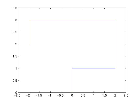
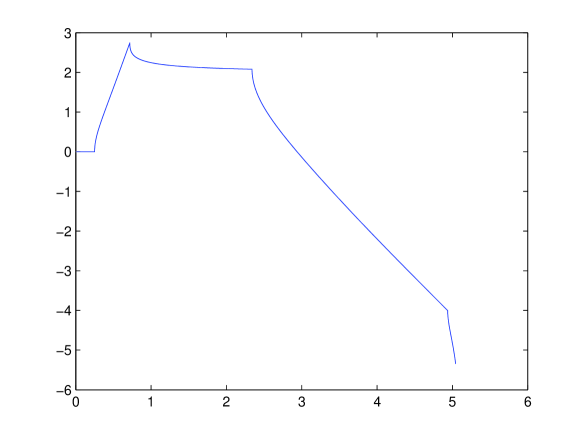
Figure 3. The example path in the upper half-plane (left) and a plot of its driving function on the $y$-axis against time on the $x$-axis (right).

It is easy to see that in this case, $t_{1}=1/4$ and $\xi$ is constantly 0 for $t\in(0,t_{1}]$. This induces the quadratic differential using (3.1):

$$Q_{t_{1}}(z)dz^{2}=\frac{z^{2}dz^{2}}{(z+1)(z-1)}.$$

Hence, we let $A_{1}(t_{1})=-1$, $A_{2}(t_{1})=1$. Also $f_{t_{1}}^{-1}(\gamma_{2})$ is a $0$-trajectory arc of $Q_{1}(z)dz^{2}$ starting from $\xi(t_{1})=0$ on $\mathbb{R}$ (by the conformal invariance of trajectories). Now note that $f_{t_{1}}^{-1}(\gamma_{2})$ makes an angle of $\pi/4$ with the positive real axis. and hence

$$f_{t_{1}+K^{-1}}\approx F_{K^{-1}}^{1/4,0}(z)$$

since $K$ is large. We can then use Newton’s method to find the preimages under the above approximation of $f_{t_{1}+K^{-1}}$ of the points $A_{1}(t_{1}),A_{2}(t_{1})$ and the 2 preimages of zero to get the points $A_{1}(t_{1}+K^{-1}),A_{2}(t_{1}+K^{-1}),C^{-}(t_{1}+K^{-1}),C^{+}(t_{1}+K^{-1})$ and hence, using (1.1), we can find $\xi(t_{1}+K^{-1})$. Then inserting this into (4.1), as detailed above we can also find $\xi(t_{1}+nK^{-1})$ and $A_{1}(t_{1}+nK^{-1}),A_{2}(t_{1}+nK^{-1}),C^{-}(t_{1}+nK^{-1}),C^{+}(t_{1}+nK^{-1})$; also, by Theorem 1.3, we can find $|\dot{\gamma}(t_{1}+nK^{-1})|$ if we let

$$t_{2}(K)=\inf\left\{n:\sum_{j=1}^{n}\frac{1}{K}|\dot{\gamma}(t_{1}+nK^{-1})|>(\text{length of }\Gamma_{2})=2\right\},$$

then $t_{2}(K)\approx t_{2}$ for $K$ large. So we just assume that $t_{2}=t_{2}(K)$. Let $A_{3}(t_{2})=C^{-}(t_{2})$ and $A_{4}(t_{2})=C^{+}(t_{2})$. Hence by (3.1),

$$Q_{t_{2}}(z)dz^{2}=\frac{(z-\xi(t_{2}))^{2}(z-A_{3}(t_{2}))dz^{2}}{(z-A_{1}(t_{2}))(z-A_{2}(t_{2}))(z-A_{4}(t_{2}))}.$$

Then, by the conformal invariance of trajectories, $f_{t_{2}}^{-1}(\Gamma_{3})$ is a $\pi/2$-trajectory of $Q_{t_{2}}(z)dz^{2}$ and also, $f_{t_{2}}^{-1}(\Gamma_{3})$, makes an angle $3\pi/4$ with $(\xi(t_{2}),\infty)$ and so

$$f_{t_{2}+K^{-1}}\approx F_{K^{-1}}^{3/4,0}(z).$$

Then, as before, we can use Newton’s method to find the preimages under the above approximation of $f_{t_{2}+K^{-1}}$ of the points $A_{1}(t_{2}),\ldots,A_{4}(t_{2})$ and the 2 preimages of $\xi(t_{2})$ to get the points $A_{1}(t_{2}+K^{-1}),\ldots,A_{4}(t_{2}+K^{-1}),C^{-}(t_{2}+K^{-1}),C^{+}(t_{2}+K^{-1})$ and hence use (1.1) to get $\xi(t_{2}+K^{-1})$. We insert these into the formula iteratively to get $\xi(t_{2}+nK^{-1})$ and $A_{1}(t_{2}+nK^{-1}),\ldots,A_{4}(t_{2}+nK^{-1}),C^{-}(t_{2}+nK^{-1}),C^{+}(t_{2}+nK^{-1})$ until $t_{2}+nK^{-1}\approx T$. Thus the end result is that we found the driving function of the first 3 steps of the slit given in Figure 3. Of course, our calculation of $\xi$ will be more accurate by taking larger $K$.  

For example, we can use the above method to calculate the driving function of any path on the square/triangle/hexagonal lattice on $\mathbb{H}$ starting from some point in $\mathbb{R}$. In fact we can calculate the driving function of a path on the square/triangle/hexagonal lattice in any polygon $D$ by mapping the half-plane conformally onto $D$ and pulling back the quadratic differential $1dw^{2}$ on $D$ to $Q(z)dz^{2}$ on $\mathbb{H}$ using the transformation law. Also note that, in general, any curve $\gamma$ can be approximated by a curve $\gamma_{\delta}$ which lies on the square lattice $\delta\mathbb{Z}^{2}$. Then it can be shown that

$$\xi_{\delta}\rightarrow\xi\text{ uniformly as }\delta\searrow 0,$$

where $\xi_{\delta}$ is the driving function of $\gamma_{\delta}$ and $\xi$ is the driving function of $\gamma$ hence, we can use the above method to calculate $\xi_{\delta}$ then take the limit as $\delta\searrow 0$ to obtain $\xi$.

Another point to note is that using the above method, we do not need to know before hand what the trajectory arc of the given quadratic differential looks like; so for arbitrary Kühnau quadratic differentials, we can use this method to plot the trajectories starting at the boundary.

We end this section by looking at what happens when the slit approaches the boundary:

Proposition 4.1.

Suppose that $\gamma:[0,T)\mapsto\overline{\mathbb{H}}$ is a simple curve such that $\gamma(0)\in\mathbb{R}$ and $\gamma(0,T)$ is a $\theta$-trajectory arc of some quadratic differential $Q(z)dz^{2}$. Then let $\xi$ be the driving function of $\gamma$. If

$$\lim_{t\uparrow T}\gamma(t)\in\mathbb{R}\cup\gamma(0,T),$$

i.e. $\gamma$ makes a loop at time $T$. Then

$$\left|\frac{d^{n}\xi}{d^{n}t}(t)\right|\rightarrow\infty\text{ as }t\nearrow T$$

for all $n=0,1,\ldots$.

Proof.

For $t\in(0,T)$, we define

$$\Gamma(t)=\{\gamma(s):s\in(t,T)\}.$$

Then $\Gamma_{t}$ is a $\theta$-trajectory arc in $H_{t}=\mathbb{H}\setminus\gamma(0,t]$ of $Q(w)dw^{2}$ and it is also a crosscut in $H_{t}$ (see [14]). Then by the conformal invariance of $\theta$-trajectories, $f_{t}^{-1}(\Gamma_{t})\subset\mathbb{H}$ is a $\theta$-trajectory arc of $Q_{t}(z)dz^{2}$. Moreover, $f_{t}^{-1}(\Gamma_{t})$ is a crosscut of $\mathbb{H}$ with one end point at $\xi(t)$ and the other end point in $\mathbb{R}$ such that either $C^{+}(t)$ or $C^{-}(t)$ is contained in the closure of the bounded component of $\mathbb{H}\setminus f_{t}^{-1}(\Gamma_{t})$. Without loss of generality, assume it is $C^{+}(t)$. Then since $\mathrm{diam}(f_{t}^{-1}(\Gamma_{t}))\rightarrow 0$ as $t\nearrow T$, we must have $\xi(t)=C^{+}(T)$ and hence by (1.2), $\dot{\xi}(t)\rightarrow\infty$ as $t\nearrow T$. Similarly, we differentiate (1.2) as mentioned in Corollary 3.1 to obtain the result for higher order derivatives. ∎

This means that as $\gamma$ gets closer and closer to making a loop, the approximation by (4.1) stops working no matter what $M$ we choose. This phenomenon can be observed in Figure 3, as we turn the last corner in $\gamma$, we can see that $\xi$ decreases faster even though the slit is not yet that close to the boundary.

5. Generalizing Theorem 1.2

5.1. Multiple slits

Suppose that $\gamma_{k}:[0,T)\rightarrow\overline{\mathbb{H}}$ for $k=1,\ldots,N$ are disjoint simple curves such that $\gamma_{k}(0)\in\mathbb{R}$ and $\gamma_{k}(0,T)\subset\mathbb{H}$. By the Riemann mapping theorem, there exists unique $f_{t}$ that map $\mathbb{H}$ conformally onto $H_{t}=\mathbb{H}\setminus\bigcup_{k=1}^{N}\gamma_{k}(0,t]$ that satisfies the hydrodynamic normalization. We can reparameterize such that

$$\bigcup_{k=1}^{N}\gamma_{k}(0,T]$$

has half-plane capacity $2t$. Then $f_{t}$ satisfies

(5.1) $$\dot{f}_{t}(z)=-2f_{t}^{\prime}(z)\left(\sum_{k=1}^{N}\frac{b_{k}(t)}{z-\xi_{k}(t)}\right),$$

where

$$\sum_{k=1}^{N}b_{k}(t)=1,$$

and $\xi_{k}(t)=f_{t}^{-1}(\gamma_{k}(t))$. See [2] for more details.

Theorem 5.1.

Suppose that $Q(w)dw^{2}$ is a Kühnau quadratic differential on $\mathbb{H}$ such that the points $\xi_{k}(0)\in\mathbb{R}$ satisfy

$$\deg_{\mathbb{H},Q}(\xi_{k}(0))=\beta_{k}\in\{0,1,2,\ldots\}$$

for all $k$. Then we can write

$$Q(w)=\left(\prod_{k=1}^{N}(w-\xi_{k}(0))^{\beta_{k}}\right)\left(\prod_{j=1}^{n}(w-a_{j})^{\alpha_{j}}\right)$$

with $a_{j}\in\mathbb{C}$ and $\alpha_{j}\in\mathbb{R}$. Then suppose that $\gamma_{k}:[0,T)\rightarrow\overline{\mathbb{H}}$ for $k=1,\ldots,N$ are disjoint simple curves such that $\gamma_{k}(0)\in\mathbb{R}$ and $\gamma_{k}(0,T)\subset\mathbb{H}$ and are parameterized as above. Then

(5.2) $$2\sum_{k=1}^{N}\xi_{k}=-\left(\sum_{k=1}^{N}(\mu_{k}^{-}C_{k}^{-}(t)+\mu_{k}^{+}C_{k}^{+}(t))\right)-\left(\sum_{j=1}^{n}\alpha_{j}A_{j}(t)\right)+\Sigma_{0},$$

and

(5.3) $$\dot{\xi}_{l}(t)=\left(\sum_{k=1,k\neq l}^{N}\frac{b_{k}(t)}{\xi_{l}(t)-\xi_{k}(t)}\right)-\frac{1}{2}\left(\sum_{k=1}^{N}\frac{\mu_{k}^{-}b_{l}(t)}{C_{k}^{-}(t)-\xi_{l}(t)}+\frac{\mu_{k}^{+}b_{l}(t)}{C_{k}^{+}(t)-\xi_{l}(t)}\right)-\frac{1}{2}\left(\sum_{j=1}^{n}\frac{\alpha_{j}b_{l}(t)}{A_{j}(t)-\xi_{l}(t)}\right)$$

for all $l\in\{1,\ldots,N\}$. Where $C_{k}^{-}(t)$ and $C_{k}^{+}(t)$ are the two preimages of $\xi_{k}(0)$ under $f_{t}$ satisfying $C_{k}^{-}(t)<C_{k}^{+}(t)$;

$$\mu_{k}^{\pm}=\deg_{H_{t},Q}(f_{t}(C_{k}^{\pm}(t)));$$

$A_{j}(t)=f_{t}^{-1}(a_{j})$; and

$$\Sigma_{0}=\left(\sum_{k=1}^{N}\beta_{k}\xi_{k}(0)\right)+\left(\sum_{j=1}^{n}\alpha_{j}a_{j}\right).$$

Proof.

By Theorem 1.1 and Lemma 2.4, we can write

$$Q(w)=\left(\prod_{k=1}^{N}(w-\xi_{k}(0))^{\beta_{k}}\right)\left(\prod_{j=1}^{n}(w-a_{j})^{\alpha_{j}}\right).$$

Then either by modifying the proof of Corollary 2.5 or iterating $N$ slit functions and applying Corollary 2.5 $N$ times, it is not too difficult to see that if we define $Q_{t}(z)$ by (3.1), then

(5.4) $$Q_{t}(z)=\left(\prod_{k=1}^{N}(z-\xi_{k}(t))^{2}(z-C_{k}^{-}(t))^{\mu_{k}^{-}}(z-C_{k}^{+}(t))^{\mu_{k}^{+}}\right)\left(\prod_{j=1}^{n}(z-A_{j}(t))^{\alpha_{j}}\right).$$

Then the proof of (5.2) is exactly the same as the proof of (1.1) in Theorem 1.2. The proof of (5.3) is more complicated. First let

$$P_{t}(z)=-2\left(\sum_{k=1}^{N}\frac{b_{k}(t)}{z-\xi_{k}(t)}\right).$$

Then (5.1) becomes

$$\dot{f}_{t}(z)=f_{t}^{\prime}(z)P_{t}(z).$$

Now take the logarithmic derivative of $Q_{t}(z)$ with respect to $z$ and $t$ separately using the definition of $Q_{t}(z)$ given by (3.1) to get

$$\frac{Q_{t}^{\prime}(z)}{Q_{t}(z)}=\frac{Q^{\prime}(f_{t}(z))f_{t}^{\prime}(z)}{Q(f_{t}(z))}+2\frac{f_{t}^{\prime\prime}(z)}{f_{t}^{\prime}(z)},$$

and

$$\frac{\dot{Q}_{t}(z)}{Q_{t}(z)} = \frac{Q^{\prime}(f_{t}(z))\dot{f}_{t}(z)}{Q(f_{t}(z))}+2\frac{\dot{f}_{t}^{\prime}(z)}{f_{t}^{\prime}(z)}$$

$$= \frac{Q^{\prime}(f_{t}(z))f_{t}^{\prime}(z)P_{t}(z)}{Q(f_{t}(z))}+2\frac{f_{t}^{\prime\prime}(z)P_{t}(z)+f_{t}^{\prime}(z)P_{t}^{\prime}(z)}{f_{t}^{\prime}(z)},$$

where we substitute (5.1) in for $\dot{f}_{t}$ to get from the first to the second line. Thus we get

(5.5) $$\frac{\dot{Q}_{t}(z)}{Q_{t}(z)}=\frac{Q_{t}^{\prime}(z)}{Q_{t}(z)}P_{t}(z)+2P_{t}^{\prime}(z).$$

So then by (5.4), we note that

$$\frac{Q^{\prime}_{t}(z)}{Q_{t}(z)}=\left(\sum_{k=1}^{N}\frac{2}{z-\xi_{k}(t)}+\frac{\mu_{k}^{-}}{z-C_{k}^{-}(t)}+\frac{\mu_{k}^{+}}{z-C_{k}^{+}(t)}\right)+\left(\sum_{j=1}^{n}\frac{\alpha_{j}}{z-A_{j}(t)}\right),$$

and

$$\frac{\dot{Q}_{t}(z)}{Q_{t}(z)}=-\left[\left(\sum_{k=1}^{N}\frac{2\dot{\xi}_{k}(t)}{z-\xi_{k}(t)}+\frac{\mu_{k}^{-}\dot{C}_{k}^{-}(t)}{z-C_{k}^{-}(t)}+\frac{\mu_{k}^{+}\dot{C}_{k}^{+}(t)}{z-C_{k}^{+}(t)}\right)+\left(\prod_{j=1}^{n}\frac{\alpha_{j}\dot{A}_{j}(t)}{z-A_{j}(t)}\right)\right].$$

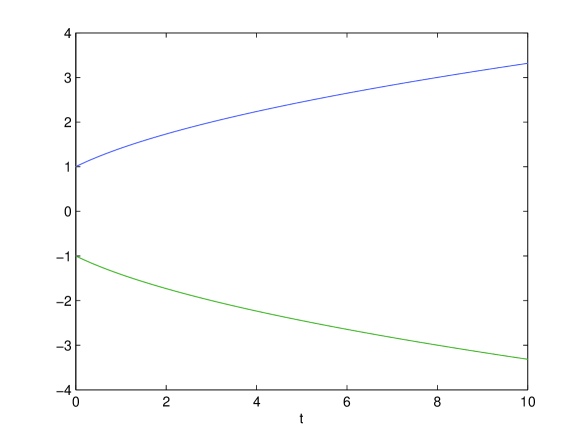
Figure 4. A plot of the two driving functions $\xi_{1}$ (top) and $\xi_{2}$ (bottom) on the $y$-axis against time on the $x$-axis.

Thus substituting this into (5.5) and comparing the coefficient of

$$\frac{1}{z-\xi_{l}(t)}$$

(i.e. the residue at $z=\xi_{l}(t)$ of both sides of (5.5)), we find that this is exactly (5.3). ∎

Similarly, we can prove a version of Theorem 1.3 and Corollary 3.1 for multiple slits. This means that we can use the method detailed in Section 4 with (5.3) to calculate the driving function for multiple $\theta_{k}$-trajectory arc slits. For example Figure 4 plots the graph of the two driving functions $\xi_{1}$ and $\xi_{2}$ in the case when $\gamma_{1}$ and $\gamma_{2}$ are 2 vertical slits starting from -1 and 1 (i.e. orthogonal trajectories of $1dz^{2}$) and growing at the same speed. Compare this with Figure 7 in [2].

5.2. Radial Loewner evolution

The chordal Loewner differential equation was introduced because the upper half-plane was an easier domain to work with for many applications but the original setting of the Loewner differential equation is in the unit disc $\mathbb{D}=\{z\in\mathbb{C}:|z|<1\}$: Suppose that $\gamma:[0,T)\mapsto\overline{\mathbb{D}}$ is a simple curve such that $\gamma(0)\in\mathbb{T}=\{z:|z|=1\}$ and $\gamma(0,T)\subset\mathbb{D}\setminus\{0\}$. Then $D_{t}=\mathbb{D}\setminus\gamma(0,t]$ is simply-connected and $0\in D_{t}$ for all $t\in(0,T)$. Hence the Riemann mapping theorem implies that there is unique conformal map $f_{t}$ mapping $\mathbb{D}$ conformally onto $D_{t}$ such that $f_{t}(0)=0$ and $f_{t}^{\prime}(0)>0$. Then Schwarz’s lemma and the Carathéodory kernel theorem implies that $f_{t}^{\prime}(0)$. is strictly decreasing and continuous so we can reparameterize such that $f_{t}^{\prime}(0)=e^{-t}$. $f_{t}^{\prime}(0)$ is sometimes called the conformal radius of $D_{t}$; hence in this case we are parameterizing by conformal radius. Then the functions $f_{t}$ satisfy the radial Loewner differential equation:

$$\dot{f}_{t}(z)=-zf_{t}^{\prime}(z)\frac{z+e^{i\xi(t)}}{z-e^{i\xi(t)}}$$

See [9] for more details.

Theorem 5.2.

Suppose that $Q(w)dw^{2}$ is a Kühnau quadratic differential on $\mathbb{D}$ such that $\deg_{Q}(0)=K\in\mathbb{Z}$ and $e^{i\xi_{0}}\in\mathbb{T}=\{|z|=1\}$ satisfies

$$\deg_{\mathbb{D},Q}\left(e^{i\xi_{0}}\right)=N\in\{0,1,2,\ldots\}$$

then we have

$$Q(w)=w^{K}(w-e^{i\xi_{0}})^{N}\left(\prod_{j=1}^{n}(w-a_{j})^{\alpha_{j}}\right),$$

where $a_{j}\in\mathbb{C}$ and $\alpha_{j}\in\mathbb{R}$. Then if $\gamma:[0,T)\mapsto\overline{\mathbb{D}}$ is a simple curve such that $\gamma(0)=e^{i\xi_{0}}$ and $\gamma(0,T)\subset\mathbb{D}\setminus\{0\}$ is a $\phi$-trajectory arc of $Q(w)dw^{2}$ in $\mathbb{D}$ that does not meet $0$ and is parameterized as above. Then we have

(5.6) $$e^{2i\xi(t)}=e^{-2t}\Pi_{0}C^{-}(t)^{-\mu^{-}}C^{+}(t)^{-\mu^{+}}\prod_{j=1}^{n}A_{j}(t)^{-\alpha_{j}},$$

and

(5.7) $$\dot{\xi}(t)=-\frac{1}{2i}\left(\mu^{-}\frac{C^{-}(t)+e^{i\xi(t)}}{C^{-}(t)-e^{i\xi(t)}}+\mu^{+}\frac{C^{+}(t)+e^{i\xi(t)}}{C^{+}(t)-e^{i\xi(t)}}+\sum_{j=1}^{n}\alpha_{j}\frac{A_{j}(t)+e^{i\xi(t)}}{A_{j}(t)-e^{i\xi(t)}}+2\right),$$

where, as usual, the functions $A_{j}(t)$ are defined by

$$A_{j}(t)=f_{t}^{-1}(a_{j})\text{ for }j=1,\ldots,n,$$

and

$$\mu^{\pm}=\deg_{D_{t},Q}(f_{t}(C^{\pm}(t))),$$

$C^{+}(t)>C^{-}(t)$ are the two preimages of $e^{i\xi_{0}}$ under $f_{t}$; and also,

$$\Pi_{0}=e^{iN\xi_{0}}\prod_{j=1}^{n}a_{j}^{\alpha_{j}}.$$

Proof.

The formula for $Q(w)$ can be obtained from Theorem 1.1 by the transformation law. We then define $Q_{t}$ by (3.1). Since the point 0 is fixed by $f_{t}$, this implies that the $\deg_{Q_{t}}(0)=\deg_{Q}(0)=K$. Thus we can apply Corollary 2.5 (again, using the transformation law) to get

$$Q_{t}(z)=z^{K}(z-e^{i\xi(t)})^{2}(z-C^{-}(t))^{\mu^{-}}(z-C^{+}(t))^{\mu^{+}}\left(\prod_{j=1}^{n}(z-A_{j}(t))^{\alpha_{j}}\right).$$

Then since by definition,

$$Q_{t}(z)=Q(f_{t}(z))f_{t}^{\prime}(z)^{2}.$$

This immediately implies (5.6) by substituting $z=0$. Then we get (5.7) in the same way as we get (1.2) from (1.1) in the proof of Theorem 1.2. ∎

As in the case of multiple slits, a version of Theorem 1.3 and Corollary 3.1 holds for this case.

5.3. Other versions of the Loewner differential equation

There are several other versions of the Loewner differential equation for simply-connected domains in the literature; the methods in this paper should work in those cases as well and the proofs should be similar to the proofs of Theorem 1.2 etc. Also, [4], [5] generalizes the Loewner differential equation to multiply-connected domains and again, some of the methods should work in these cases possibly using methods in [1] to extend Theorem 1.1 to multiply-connected domains. Finally, even if we consider general 2-dimensional growth processes given by the Loewner-Kufarev differential equation (see Chapter 6 of [13]), some of the methods in this paper should still be applicable.

Acknowledgement.

The author would like to express his gratitude to his supervisor Dr. T. K. Carne for his constant guidance and helpful discussion when writing this paper.

References

- [1] D. Crowdy. The Schwarz-Christoffel mapping to bounded multiply connected polygonal domains. Proc. R. Soc. Lond. Ser. A Math. Phys. Eng. Sci., 461(2061):2653–2678, 2005.
- [2] W. Kager, B. Nienhuis, and L. P. Kadanoff. Exact solutions for Loewner evolutions. J. Statist. Phys., 115(3-4):805–822, 2004.
- [3] T. Kennedy. Computing the Loewner driving process of random curves in the half plane. arXiv:math/0702071v1
- [4] Y. Komatu. Untersuchungen über konforme Abbildung von zweifach zusammenhängenden Gebieten. Proc. Phys.-Math. Soc. Japan (3), 25:1–42, 1943.
- [5] Y. Komatu. On conformal slit mapping of multiply-connected domains. Proc. Japan Acad., 26(7):26–31, 1950.
- [6] R. Kühnau. Über die analytische Darstellung von Abbildungsfunktionen insbesondere von Extremalfunktionen der Theorie der konformen Abbildung. J. Reine Angew. Math., 228:93–132, 1967.
- [7] G. F. Lawler. Conformally invariant processes in the plane. American Mathematical Society, USA, 2005.
- [8] J. R. Lind. A sharp condition for the Loewner equation to generate slits. Ann. Acad. Sci. Fenn. Math., 30(1):143–158, 2005.
- [9] K. Löwner. Untersuchungen über schlichte konforme Abbildungen des Einheitskreises, I. Math. Ann., 89, 1923.
- [10] D. E. Marshall and S. Rohde. The Loewner differential equation and slit mappings. J. Amer. Math. Soc., 18(4):763–778 (electronic), 2005.
- [11] D. E. Marshall and S. Rohde. Convergence of the zipper algorithm for conformal mapping. preprint, 2006.
- [12] Z. Nehari. Conformal mapping. Dover Publications, New York, 1982.
- [13] C. Pommerenke. Univalent functions. Vandenhoeck & Ruprecht, Göttingen, 1975. With a chapter on quadratic differentials by Gerd Jensen, Studia Mathematica/Mathematische Lehrbücher, Band XXV.
- [14] C. Pommerenke. Boundary behaviour of conformal maps. Springer-Verlag, Berlin, 1992.
- [15] O. Schramm. Scaling limits of loop-erased random walks and uniform spanning trees. Israel J. Math., 118:221–288, 2000.
- [16] K. Strebel. Quadratic differentials. Springer-Verlag, Berlin, 1984.