USTC-ICTS-07-02

Probing $\alpha$-Vacua of Black Holes in LHC

Tower Wang

Institute of Theoretical Physics, Chinese Academy of Sciences,

P. O. Box 2735 Beijing 100080, China

Interdisciplinary Center for Theoretical Study,

University of Science and Technology of China,

Hefei, Anhui 230026, China

wangtao218@itp.ac.cn

Abstract

Motivated by the idea of $\alpha$-vacua in Schwarzschild spacetime, we studied the deformed spectrum of Hawking radiation. Such a deformation would leave signatures on the small black hole evaporation in LHC because their vacuum deviates from the Unruh state.

For massive scalar fields there is a family of de Sitter-invariant states, including the Hartle-Hawking vacuum state as a special case [1, 2]. These states are well known as the so-called $\alpha$-vacua because they are related to Hartle-Hawking vacuum by a new parameter $\alpha$ [2]. The choice of physical vacuum from these states might be imprinted on the spectrum of CMBR (see e.g. [3]). The application of $\alpha$-vacua to cosmological dark energy can be found in [4] as a recent review.

Starting with Hartle-Hawking vacuum, Chamblin and Michelson in [6] constructed the $\alpha$-vacua of scalar field in Schwarzschild, Schwarzschild-dS and Schwarzschild-AdS black hole spacetimes. However, it is generally conceived that at late times, a black hole formed from gravitational collapse is well-approximated by an eternal black hole with the scalar field in the Unruh state [9], rather than in the Hartle-Hawking state [8]. On the other hand, assuming large extra dimensions and TeV Plank scale, small black holes would be produced and decay in LHC [11, 12, 13], thus provide the first experimental test of Hawking’s radiation hypothesis [7]. Their sudden evaporation takes place not very long after the formation, so naturally their vacuum deviates from the Unruh state. Fortunately, since the discussion in [6] does not depend heavily on the details of vacuum with which one starts, the $\alpha$-vacua from the Unruh state can also be constructed, in hopes of characterizing such a deviation with new parameters.

In this paper, we explore the modified spectrum of Hawking radiation for scalars, considering effects of the $\alpha$-vacua of Schwarzschild spacetime. If small black holes are indeed produced in LHC abundantly, such a modification may leave observable fingerprints on their evaporation spectrum.

Before getting the spectrum, we would like to work over some details about the $\alpha$-vacua. We first introduce a set of global coordinates of Schwarzschild spacetime, by embedding it into $\mathcal{M}^{6,1}$. The global coordinates are a byproduct of this paper, in which the symmetry under antipodal map is more manifest than in other coordinates. After partly solving the Klein-Gordon equation, we then deduce a more exact expression of $\alpha$-vacua, which relates to the usual Hartle-hawking vacuum modes via a trivial (nonmixing) Bogoliubov transformation and a Mottola-Allen transformation.

Subsequently, in order to search some signatures of $\alpha$-vacua in LHC phenomenologically, we turn to the Unruh state and the corresponding $\alpha$-vacua, and derive the evaporation spectrum following the standard procedure, i.e., by picking up the Bogoliubov coefficients. The spectrum depends on two new parameters $\alpha$ and $\gamma$. When $\alpha\neq 0$, it deviates from ordinary greybody spectrum of Hawking radiation. So at the end of this paper, we discussed implications of our result for small black holes in large extra dimensional scenarios.

In static coordinates, the Schwarzschild metric is

$$ds^{2}=-\left(1-\frac{2M}{r}\right)dt^{2}+\left(1-\frac{2M}{r}\right)^{-1}dr^{2}+r^{2}(d\theta^{2}+\sin^{2}\theta d\varphi^{2}).$$ (1)

It can be embedded into $\mathcal{M}^{6,1}$

$$ds^{2}=-dX^{2}_{0}+dX^{2}_{1}+dX^{2}_{2}+dX^{2}_{3}+dX^{2}_{4}+dX^{2}_{5}+dX^{2}_{6}$$ (2)

by setting [5, 6]

$$X_{1}=r\sin\theta\cos\varphi,\leavevmode\nobreak\ \leavevmode\nobreak\ \leavevmode\nobreak\ \leavevmode\nobreak\ X_{2}=r\sin\theta\sin\varphi,\leavevmode\nobreak\ \leavevmode\nobreak\ \leavevmode\nobreak\ \leavevmode\nobreak\ X_{3}=r\cos\theta,$$

$$X_{4}=-2M\sqrt{\frac{2M}{r}}+4M\sqrt{\frac{r}{2M}},\leavevmode\nobreak\ \leavevmode\nobreak\ \leavevmode\nobreak\ \leavevmode\nobreak\ X_{5}=2\sqrt{3}M\sqrt{\frac{2M}{r}},$$

$$X_{6}=4M\sqrt{1-\frac{2M}{r}}\cosh\left(\frac{t}{4M}\right),\leavevmode\nobreak\ \leavevmode\nobreak\ \leavevmode\nobreak\ \leavevmode\nobreak\ X_{0}=4M\sqrt{1-\frac{2M}{r}}\sinh\left(\frac{t}{4M}\right).$$ (3)

The spacetime outside the horizon of Schwarzschild black hole is given as the algebraic variety determined by the three polynomials [5, 6]

$$\frac{4}{3}X_{5}^{2}+X_{6}^{2}-X_{0}^{2} = 16M^{2},$$

$$X_{5}^{4}(X_{1}^{2}+X_{2}^{2}+X_{3}^{2}) = 576M^{6},$$

$$\sqrt{3}X_{4}X_{5}+X_{5}^{2} = 24M^{2}.$$ (4)

The global coordinates are related to static coordinates via

$$\left(e^{\frac{t}{2M}},r,\theta,\varphi\right)_{\mathrm{static}}\rightarrow\left(\frac{\cos\sigma+\tanh\tau}{\cos\sigma-\tanh\tau},\frac{2M}{\cosh^{2}\tau\sin^{2}\sigma},\theta,\varphi\right)_{\mathrm{global}},$$ (5)

which is resulted from the definition

$$X_{1}=\frac{2M\sin\theta\cos\varphi}{\cosh^{2}\tau\sin^{2}\sigma},\leavevmode\nobreak\ \leavevmode\nobreak\ \leavevmode\nobreak\ \leavevmode\nobreak\ X_{2}=\frac{2M\sin\theta\sin\varphi}{\cosh^{2}\tau\sin^{2}\sigma},\leavevmode\nobreak\ \leavevmode\nobreak\ \leavevmode\nobreak\ \leavevmode\nobreak\ X_{3}=\frac{2M\cos\theta}{\cosh^{2}\tau\sin^{2}\sigma},$$

$$X_{4}=-2M\cosh\tau\sin\sigma+\frac{4M}{\cosh\tau\sin\sigma},\leavevmode\nobreak\ \leavevmode\nobreak\ \leavevmode\nobreak\ \leavevmode\nobreak\ X_{5}=2\sqrt{3}M\cosh\tau\sin\sigma,$$

$$X_{6}=4M\cosh\tau\cos\sigma,\leavevmode\nobreak\ \leavevmode\nobreak\ \leavevmode\nobreak\ \leavevmode\nobreak\ X_{0}=4M\sinh\tau,$$ (6)

and gives the form of metric

$$ds^{2} = \frac{16M^{2}}{\cosh^{6}\tau\sin^{6}\sigma}\{\sin^{2}\sigma[\sinh^{2}\tau(1+\cosh^{2}\tau\sin^{2}\sigma)-\cosh^{4}\tau\sin^{4}\sigma]d\tau^{2}$$ (7)

$$+\cosh^{2}\tau[\cos^{2}\sigma(1+\cosh^{2}\tau\sin^{2}\sigma+\cosh^{4}\tau\sin^{4}\sigma)+\cosh^{6}\tau\sin^{6}\sigma]d\sigma^{2}$$

$$+2\sinh\tau\cosh\tau\sin\sigma\cos\sigma(1+\cosh^{2}\tau\sin^{2}\sigma+\cosh^{4}\tau\sin^{4}\sigma)d\tau d\sigma\}$$

$$+\frac{4M^{2}}{\cosh^{4}\tau\sin^{4}\sigma}(d\theta^{2}+\sin^{2}\theta d\varphi^{2}).$$

Clearly the global coordinates presented above are quite similar to but more complicated than those for de Sitter spacetime [16].

Correspondingly the measure is

$$\sqrt{-g}=\left|\frac{64M^{4}\sin\theta}{\cosh^{6}\tau\sin^{7}\sigma}\right|,$$ (8)

while the non-vanishing components of contravariant metric tensor are

$$g^{\tau\tau} = -\frac{1}{16M^{2}}[\cos^{2}\sigma(1+\cosh^{2}\tau\sin^{2}\sigma+\cosh^{4}\tau\sin^{4}\sigma)+\cosh^{6}\tau\sin^{6}\sigma],$$

$$g^{\tau\sigma} = g^{\sigma\tau}=\frac{\sinh\tau\sin\sigma\cos\sigma}{16M^{2}\cosh\tau}(1+\cosh^{2}\tau\sin^{2}\sigma+\cosh^{4}\tau\sin^{4}\sigma),$$

$$g^{\sigma\sigma} = -\frac{\sin^{2}\sigma}{16M^{2}\cosh^{2}\tau}[\sinh^{2}\tau(1+\cosh^{2}\tau\sin^{2}\sigma)-\cosh^{4}\tau\sin^{4}\sigma],$$

$$g^{\theta\theta} = \frac{\cosh^{4}\tau\sin^{4}\sigma}{4M^{2}},\leavevmode\nobreak\ \leavevmode\nobreak\ \leavevmode\nobreak\ \leavevmode\nobreak\ g^{\varphi\varphi}=\frac{\cosh^{4}\tau\sin^{4}\sigma}{4M^{2}\sin^{2}\theta}.$$ (9)

The covariant Klein-Gordon equation

$$(\Box_{x}-\mu^{2})\Phi(x)=\frac{1}{\sqrt{-g}}\partial_{\mu}(\sqrt{-g}g^{\mu\nu}\partial_{\nu}\Phi)-\mu^{2}\Phi=0$$ (10)

in global coordinates is too complicated to be fully solved by brute force. However, we can still get some details from it as follows.

In terms of global coordinates, the antipodal map [2, 6] $x\rightarrow x_{A}$ reads

$$(\tau,\sigma,\theta,\varphi)\rightarrow(-\tau,\pi-\sigma,\pi-\theta,\varphi\pm\pi).$$ (11)

It is easy to see the metric (7) is manifestly invariant under this antipodal transformation and further

$$(\Box_{x}-\mu^{2})G_{0}^{(1)}(x,y)=0$$

$$\Rightarrow (\Box_{x_{A}}-\mu^{2})G_{0}^{(1)}(x_{A},y)=(\Box_{x}-\mu^{2})G_{0}^{(1)}(x_{A},y)=0$$ (12)

for the Hadamard function $G_{0}^{(1)}(x,y)$. That is to say, the Hadamard functions $G_{0}^{(1)}(x,y)$ and $G_{0}^{(1)}(x_{A},y)$ satisfy the same equation. This property is most manifest in global coordinates. We emphasize the property here and confirm the existence of a complete set of orthonormal modes obeying

$$\phi_{\omega,l,m}(x_{A})=\phi^{*}_{\omega,l,m}(x)$$ (13)

in the following, because they play important roles in proving that the $\alpha$-vacua respect symmetries of the spacetime [2, 6]. For de Sitter spacetime, the symmetry is the $O(1,4)$ group. While for Schwarzchild spacetime, it is the “$CPT$” invariance introduced in [5] and recounted in [6].

In [6], it was argued that one can choose the modes satisfying (13) because the equation of motion is invariant under complex conjugation and under the antipodal map. It seems to me this argument guarantees only the existence of certain special solution of differential equation (10) which satisfies $\Phi(x_{A})=\Phi^{*}(x)$, rather than the existence of a set of Hartle-Hawking vacuum modes $\phi_{\omega,l,m}$ satisfying (13). We would like to fill this gap and make the argument in [6] more solid, by precisely constructing these modes of Hartle-Hawking vacuum.

Our construction will be based on some results presented in [17]. In the book [17], a complete set of Hartle-Hawking modes $\hat{\phi}^{(1)}_{\omega,l,m}$, $\hat{\phi}^{(2)}_{\omega,l,m}$, $\hat{\phi}^{(3)}_{\omega,l,m}$ and $\hat{\phi}^{(4)}_{\omega,l,m}$ has been constructed. These modes are orthonormal and meet conditions [17]

$$\hat{\phi}^{(1)}_{\omega,l,m}(-U,-V,\theta,\varphi) = \hat{\phi}^{(2)*}_{\omega,l,m}(U,V,\theta,\varphi),$$

$$\hat{\phi}^{(3)}_{\omega,l,m}(-U,-V,\theta,\varphi) = \hat{\phi}^{(4)*}_{\omega,l,m}(U,V,\theta,\varphi).$$ (14)

Here $U$, $V$ are Kruskal coordinates. In our global coordinates, the conditions are translated into

$$\hat{\phi}^{(1)*}_{\omega,l,m}(-\tau,\pi-\sigma,\theta,\varphi) = \hat{\phi}^{(2)}_{\omega,l,m}(\tau,\sigma,\theta,\varphi),$$

$$\hat{\phi}^{(3)*}_{\omega,l,m}(-\tau,\pi-\sigma,\theta,\varphi) = \hat{\phi}^{(4)}_{\omega,l,m}(\tau,\sigma,\theta,\varphi).$$ (15)

At the same time, it is trivial to show the factorization

$$\hat{\phi}^{(i)}_{\omega,l,m}(x)=\hat{f}^{(i)}_{\omega,l,m}(\tau,\sigma)Y_{l,m}(\theta,\varphi),\leavevmode\nobreak\ \leavevmode\nobreak\ \leavevmode\nobreak\ \leavevmode\nobreak\ i=1,2,3,4$$ (16)

is valid utilizing equation (10). We stress that such a factorization is valid in the whole spacetime. On boundaries $\mathcal{H}^{\pm}$ especially, the book [17] gave analytic expressions of $\hat{\phi}^{(i)}_{\omega,l,m}$, and one can show they are factorized as (16) indeed. Combining (S0.Ex15), (16) and the following formula for spherical harmonic functions

$$Y_{l,m}(\pi-\theta,\varphi\pm\pi)=(-1)^{l}Y_{l,m}(\theta,\varphi)$$ (17)

together, we can check the relations

$$\hat{\phi}^{(1)*}_{\omega,l,m}(x_{A}) = (-1)^{l}\hat{\phi}^{(2)}_{\omega,l,m}(x),$$

$$\hat{\phi}^{(3)*}_{\omega,l,m}(x_{A}) = (-1)^{l}\hat{\phi}^{(4)}_{\omega,l,m}(x),$$ (18)

and construct a set of new orthonormal modes $\phi_{\omega,l,m}$ by the trivial Bogoliubov transformation [2]

$$\phi^{(1)}_{\omega,l,m}(x) = \frac{1}{\sqrt{2}}e^{i\pi l/2}[\hat{\phi}^{(1)}_{\omega,l,m}(x)+\hat{\phi}^{(2)}_{\omega,l,m}(x)],$$

$$\phi^{(2)}_{\omega,l,m}(x) = \frac{1}{\sqrt{2}}e^{i\pi(l+1)/2}[\hat{\phi}^{(1)}_{\omega,l,m}(x)-\hat{\phi}^{(2)}_{\omega,l,m}(x)],$$

$$\phi^{(3)}_{\omega,l,m}(x) = \frac{1}{\sqrt{2}}e^{i\pi l/2}[\hat{\phi}^{(3)}_{\omega,l,m}(x)+\hat{\phi}^{(4)}_{\omega,l,m}(x)],$$

$$\phi^{(4)}_{\omega,l,m}(x) = \frac{1}{\sqrt{2}}e^{i\pi(l+1)/2}[\hat{\phi}^{(3)}_{\omega,l,m}(x)-\hat{\phi}^{(4)}_{\omega,l,m}(x)].$$ (19)

The modes (21) form a complete set of orthonormal modes. In particular,

1. $\phi^{(i)}_{\omega,l,m}(x_{A})=\phi^{(i)*}_{\omega,l,m}(x)$.

2. $(\phi^{(i)}_{\omega,l,m},\phi^{(i^{\prime})}_{\omega^{\prime},l^{\prime},m^{\prime}})=\delta_{i,i^{\prime}}\delta_{\omega,\omega^{\prime}}\delta_{l,l^{\prime}}\delta_{m,m^{\prime}}$ and $(\phi^{(i)}_{\omega,l,m},\phi^{(i^{\prime})*}_{\omega^{\prime},l^{\prime},m^{\prime}})=0$.

3. The set of $\phi_{\omega,l,m}$ is complete and spans the space of $\hat{\phi}_{\omega,l,m}$.

The $\alpha$-vacua are constructed from this set of modes by a Mottola-Allen transformation [2, 6]

$$\tilde{\phi}^{(i)}_{\omega,l,m}(x)=\cosh\alpha\phi^{(i)}_{\omega,l,m}(x)+e^{i\gamma}\sinh\alpha\phi^{(i)*}_{\omega,l,m}(x),\leavevmode\nobreak\ \leavevmode\nobreak\ \leavevmode\nobreak\ \leavevmode\nobreak\ \alpha\geq 0,\leavevmode\nobreak\ \leavevmode\nobreak\ -\pi<\gamma\leq\pi.$$ (20)

One should notice that $\hat{\phi}^{(i)}_{\omega,l,m}(x)$ and $\phi^{(i)}_{\omega,l,m}(x)$ are of positive frequencies with respect to the affine parameters on $\mathcal{H}^{\pm}$. However, this is not true for $\tilde{\phi}^{(i)}_{\omega,l,m}(x)$ since the transformation (20) mixes modes of the same frequency but with different sign. Or equivalently, from another point of view based on (13), it mixes modes on the antipodal points $x$ and $x_{A}$. The modes (20) are taken as a new “vacuum” state [1, 2] because this transformation is (the Bogoliubov coefficients are) frequency independent and preserves orthonormality.

The scalar field in (10) may be decomposed in different bases if we consider different vacua,

$$\Phi(x) = \sum_{i,\omega,l,m}\left[a^{(i)}_{\omega,l,m}\phi^{(i)}_{\omega,l,m}(x)+a^{(i){\dagger}}_{\omega,l,m}\phi^{(i)*}_{\omega,l,m}(x)\right]$$ (21)

$$= \sum_{i,\omega,l,m}\left[\tilde{a}^{(i)}_{\omega,l,m}\tilde{\phi}^{(i)}_{\omega,l,m}(x)+\tilde{a}^{(i){\dagger}}_{\omega,l,m}\tilde{\phi}^{(i)*}_{\omega,l,m}(x)\right].$$

The properties (S0.Ex13) and (13) are the major tricks to study properties of two-point functions, and to prove that $\alpha$-vacua respect the symmetries of the spacetime [2, 6]. For example, equation (13) leads to a relation between Hadamard function $G_{\alpha\gamma}^{(1)}(x,y)$ for $\alpha$-vacua and $G_{0}^{(1)}(x,y)$, $D_{0}(x,y)$ for Hartle-Hawking vacuum,

$$G_{\alpha\gamma}^{(1)}(x,y)=\cosh(2\alpha)G_{0}^{(1)}(x,y)+\cos\gamma\sinh(2\alpha)G_{0}^{(1)}(x_{A},y)-\sin\gamma\sinh(2\alpha)D_{0}(x_{A},y).$$ (22)

From (13) it is clear that $G_{0}^{(1)}(x,y)$ and $G_{0}^{(1)}(x_{A},y)$ obey the same equation of motion and hence respect symmetries of the spacetime. Therefore, $G_{\alpha\gamma}^{(1)}(x,y)$ is $CPT$ [5, 6] invariant for $\alpha$-vacua with $\gamma=0,\pi$. As explained in [2] and reiterated in [6], the $\alpha$-vacua with $\sin\gamma\neq 0$ break the time-reversal symmetry, to which we will come back later when discussing small black holes in LHC.

In the previous part we focused on two tasks:

1. making it more manifest that $G_{0}^{(1)}(x_{A},y)$ obeys the same equation as that of $G_{0}^{(1)}(x,y)$, thus preserves the symmetries of the Schwarzschild spacetime; and

2. establishing a complete set of orthonormal modes satisfying (13).

Global coordinates (7) of Scharzschild spacetime were a byproduct during our research. The coordinates may be not necessary here, but facilitate the first task in a way. Their physical implications and applications in various aspects of Schwarzschild black hole remain unclear, which we would like to study elsewhere in the future.

In the following, to be brief, we will work in the matrix formalism. That is, we will write a basis of modes in a column matrix and multiply it by a square matrix to represent the Bogoliubov transformation. For example, the trivial Bogoliubov transformation (21) will be written concisely,

$$\phi_{i}=P_{ij}\hat{\phi}_{j},$$ (23)

where the collective subscript $i$ or $j$ denotes the complete set of quantum numbers $\omega$,$l$,$m$ and superscripts ($i$) that must be specified to describe a mode. Or even more compactly,

$$\phi=P\hat{\phi}.$$ (24)

Likewise, the Mottola-Allen transformation (20) will be denoted in the form

$$\tilde{\phi}=\cosh\alpha\phi+e^{i\gamma}\sinh\alpha\phi^{*},\leavevmode\nobreak\ \leavevmode\nobreak\ \leavevmode\nobreak\ \leavevmode\nobreak\ \alpha\geq 0,\leavevmode\nobreak\ \leavevmode\nobreak\ -\pi<\gamma\leq\pi.$$ (25)

In the above, we have been dealing with the Hartle-Hawking type $\alpha$-vacua, and focusing on some theoretical problems. In the following, we will turn to a relatively independent issue – a phenomenological problem: calculating the evaporation spectrum for the Unruh vacuum and those for its $\alpha$-vacua correspondingly.

For Unruh vacuum, the procedure is standard [9, 18]. If we use $\psi^{\prime}_{i}$ to label the positive frequency modes on $\Im^{+}$ and $\psi_{i}$ to label the positive frequency modes on $\Im^{-}$, then the Bogoliubov transformation $\psi_{i}\rightarrow\psi^{\prime}_{i}$, i.e., $a_{i}\rightarrow a^{\prime}_{i}$ can be written as

$$\psi^{\prime}=A\psi+B\psi^{*},$$ (26)

or namely

$$a=a^{\prime}A+a^{\prime{\dagger}}B^{*},$$ (27)

in which $A$ and $B$ are Bogoliubov transformation matrices, while $a$ and $a^{\prime}$ are row matrices with elements $a_{i}$ and $a^{\prime}_{i}$ respectively. A solution of the field equation (10) can be expanded as

$$\Phi(x)=\sum_{i}(a_{i}\psi_{i}+a^{{\dagger}}_{i}\psi^{*}_{i})=\sum_{i}(a^{\prime}_{i}\psi^{\prime}_{i}+a_{i}^{\prime{\dagger}}\psi^{\prime*}_{i}).$$ (28)

It has been proved in [18] that there is a relation between the Bogoliubov coefficients

$$B_{ij}=-e^{-\omega_{i}/(2T_{H})}A_{ij},$$ (29)

and the late time particle flux through $\Im^{+}$ given a vacuum on $\Im^{-}$ is determined by [18]

$$\left(BB^{{\dagger}}\right)^{*}_{ii}=\frac{1}{e^{\omega_{i}/T_{H}}-1}.$$ (30)

In (4+n)-dimensions [10], the Hawking temperature can be traded for the black hole radius [13],

$$T_{H}=\frac{n+1}{4\pi r_{H}}.$$ (31)

Taking into consideration of greybody factor, the spectrum of energy flux has the form

$$\frac{dE(\omega)}{dt}=\sum_{l}\sigma_{l,n}(\omega)\frac{\omega}{e^{\omega/T_{H}}-1}\frac{dk^{n+3}}{(2\pi)^{n+3}}.$$ (32)

At low energy $\omega r_{H}\ll 1$, an analytic expression for greybody factor $\sigma_{l,n}$ has been derived in [14, 15]. In large extra dimensional scenarios, small black holes may emit scalar fields in the bulk as well as on the brane. Our attention in this paper will be “localized” on the brane with the help of analytic formulas given in [14, 15], although the calculation in the bulk can be accomplished in a similar way. In the massless particle approximation, corresponding to Unruh vacuum (30), the low energy scalar spectrum on the brane is [14, 15]

$$\frac{d^{2}E(\omega)}{d\omega dt}=r_{H}^{-1}\sum_{l}\frac{(2l+1)\Gamma(\frac{l+1}{n+1})^{2}\Gamma(1+\frac{l}{n+1})^{2}}{(n+1)^{2}\Gamma(\frac{1}{2}+l)^{2}\Gamma(1+\frac{2l+1}{n+1})^{2}}\left(\frac{\omega r_{H}}{2}\right)^{2l}\frac{2(\omega r_{H})^{3}}{e^{4\pi\omega r_{H}/(n+1)}-1}.$$ (33)

For the $\alpha$-vacua constructed from the Unruh state, we should consider the following series of transformations

$$\tilde{\psi}_{i}\rightarrow\psi_{i}\rightarrow\psi^{\prime}_{i},$$

$$\tilde{a}_{i}\rightarrow a_{i}\rightarrow a^{\prime}_{i}.$$ (34)

In other words, we take the $\alpha$ state

$$\tilde{\psi}=\cosh\alpha\psi+e^{i\gamma}\sinh\alpha\psi^{*},\leavevmode\nobreak\ \leavevmode\nobreak\ \leavevmode\nobreak\ \leavevmode\nobreak\ \alpha\geq 0,\leavevmode\nobreak\ \leavevmode\nobreak\ -\pi<\gamma\leq\pi$$ (35)

as the physical vacuum on $\Im^{-}$. Inversion of (35) leads to

$$\psi=\cosh\alpha\tilde{\psi}-e^{i\gamma}\sinh\alpha\tilde{\psi}^{*}.$$ (36)

At the same time, one can also formally write

$$\psi^{\prime}=\tilde{A}\tilde{\psi}+\tilde{B}\tilde{\psi}^{*},\leavevmode\nobreak\ \leavevmode\nobreak\ \leavevmode\nobreak\ \leavevmode\nobreak\ \tilde{\psi}=\tilde{A}^{\prime}\psi^{\prime}+\tilde{B}^{\prime}\psi^{\prime*}.$$ (37)

The expected number of particles in the $i$th mode is related to $\left(\tilde{B}\tilde{B}^{{\dagger}}\right)^{*}_{ii}$. From the relations (26), (36) and (37), one immediately gets

$$\psi^{\prime}=(A\cosh\alpha-Be^{-i\gamma}\sinh\alpha)\tilde{\psi}+(B\cosh\alpha-Ae^{i\gamma}\sinh\alpha)\tilde{\psi}^{*},$$ (38)

thus

$$\tilde{B}=B\cosh\alpha-Ae^{i\gamma}\sinh\alpha.$$ (39)

Multiplied by

$$\tilde{B}^{{\dagger}}=B^{{\dagger}}\cosh\alpha-A^{{\dagger}}e^{-i\gamma}\sinh\alpha,$$ (40)

it gives

$$\tilde{B}\tilde{B}^{{\dagger}}=\cosh^{2}\alpha\left(BB^{{\dagger}}\right)+\sinh^{2}\alpha\left(AA^{{\dagger}}\right)-\sinh\alpha\cosh\alpha[e^{i\gamma}\left(AB^{{\dagger}}\right)+e^{-i\gamma}\left(BA^{{\dagger}}\right)].$$ (41)

As a consistency check, when $\alpha=0$, apparently it reduces to the expected form $\tilde{B}\tilde{B}^{{\dagger}}|_{\alpha=0}=BB^{{\dagger}}$. In virtue of (29), (30) and (31), one can simplify the diagonal entries in (41) and write down

$$\left(\tilde{B}\tilde{B}^{{\dagger}}\right)^{*}_{ii}=\frac{\sinh^{2}\alpha e^{4\pi\omega_{i}r_{H}/(n+1)}+\cos\gamma\sinh(2\alpha)e^{2\pi\omega_{i}r_{H}/(n+1)}+\cosh^{2}\alpha}{e^{4\pi\omega_{i}r_{H}/(n+1)}-1}.$$ (42)

The absorption amplitude and greybody factor are caused by the traversal of emitted particles in the gravitational background. They are independent of the initial conditions, i.e., independent of the vacuum we choose on $\Im^{-}$. As a result, given an $\alpha$ state as the vacuum on $\Im^{-}$, at the late time, the low energy flux through $\Im^{+}$ is

$$\frac{d^{2}E(\omega)}{d\omega dt} = r_{H}^{-1}\sum_{l}\frac{(2l+1)\Gamma(\frac{l+1}{n+1})^{2}\Gamma(1+\frac{l}{n+1})^{2}}{(n+1)^{2}\Gamma(\frac{1}{2}+l)^{2}\Gamma(1+\frac{2l+1}{n+1})^{2}}\left(\frac{\omega r_{H}}{2}\right)^{2l}2(\omega r_{H})^{3}$$ (43)

$$\times\frac{\sinh^{2}\alpha e^{4\pi\omega r_{H}/(n+1)}+\cos\gamma\sinh(2\alpha)e^{2\pi\omega r_{H}/(n+1)}+\cosh^{2}\alpha}{e^{4\pi\omega r_{H}/(n+1)}-1}.$$

For high energy emissions $\omega r_{H}\gg 1$, equation (43) predicts a divergent energy flux. This suggests the breakdown of (42) and (43) at very high energy. Indeed, during derivation of the spectrum, we have neglected backreactions to the black hole, which are supposed to be small at low energy. In the high energy region, especially for small black holes, the backreaction effect of the particle emission will be large, so the spectrum (42) together with (43) cannot be trusted there any more.

Assuming large extra dimensions and TeV Plank scale, in [11, 12, 13], it has been proposed that small black holes of TeV scale masses would be produced in LHC and provide the first experimental test of Hawking’s radiation hypothesis. On the one hand, the lifetime of the small black holes in this scenario is of order

$$\tau\sim M_{p}^{*-1}\left(\frac{M}{M_{p}^{*}}\right)^{\frac{n+3}{n+1}}\sim r_{H}\left(\frac{M}{M_{p}^{*}}\right)^{\frac{n+2}{n+1}}$$ (44)

or typically $10^{-26}$ second [12, 15], much shorter than that of ordinary black holes in astrophysics. On the other hand, for a black hole formed by collapse, at a sufficiently long time after its formation, the Unruh state serves as a good boundary condition of Green’s function. While not long after its formation, the boundary condition depends on details of the collapse. If we introduce the $\alpha$-vacua (35) as a new boundary condition, there are two additional parameters $\alpha$ and $\gamma$, which would capture some universal features of the black hole formation in LHC and characterize the deviation of the vacuum from the Unruh vacuum. In this sense, the physical values of $\alpha$ and $\gamma$ cannot be determined theoretically. However, we observe that for non-eternal black holes, possibly the value of $\alpha$ depends on their lifetime. Specifically, we guess that $\alpha$ increases with respect to the ratio $\frac{M_{p}^{*}}{M}$, and vanishes in the limit $\frac{M_{p}^{*}}{M}\rightarrow 0$. In large extra dimensional scenarios, for small black holes produced in LHC, the ratio is of order $1<\frac{M_{p}^{*}}{M}\lesssim 10$, thus we can take $\alpha$ as a parameter of constant. If $\alpha$ is large enough, in the low energy region $\omega r_{H}\ll 1$, the greybody profile of Hawking radiation will be deformed according to (43). Schwarzschild phase is an important stage during the evaporation of small black holes. If a non-vanishing value of $\alpha$ is indeed physical for these black holes, signatures of (43) must be imprinted on the evaporation spectrum, thus can be found out by a detailed study of small black hole decay.

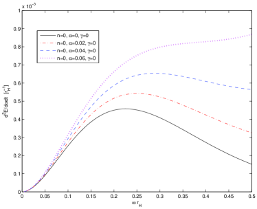
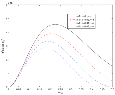
Figure 1: The scalar energy flux $\frac{d^{2}E(\omega)}{d\omega dt}$ on the brane as a function of $\omega r_{H}$ with $n=0$, $\alpha=0$ (black solid lines), $0.02$ (red dash-dotted lines), $0.04$ (blue dashed lines), $0.06$ (magenta dotted lines) and $\gamma=0$ (the left graph), $\pi$ (the right graph).

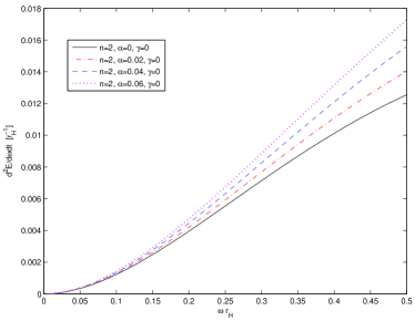
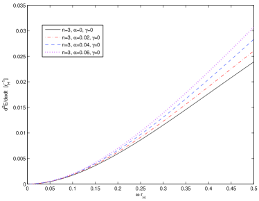
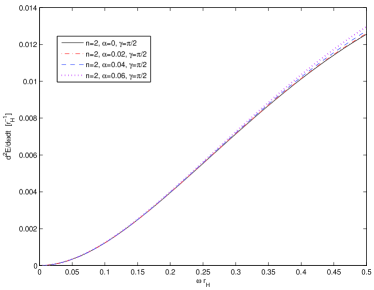
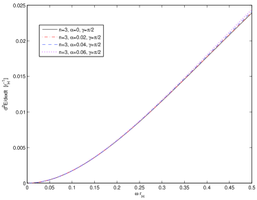
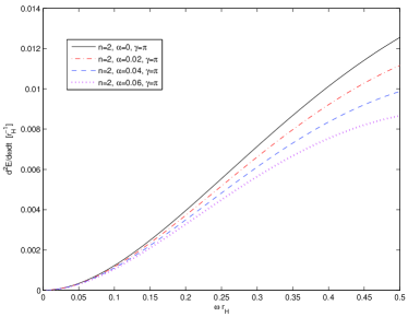
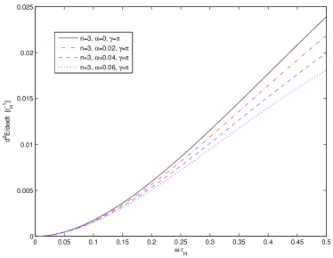
Figure 2: The scalar energy flux $\frac{d^{2}E(\omega)}{d\omega dt}$ on the brane as a function of $\omega r_{H}$ with $n=2$ (the left graphs), $n=3$ (the right graphs), $\alpha=0$ (black solid lines), $0.02$ (red dash-dotted lines), $0.04$ (blue dashed lines), $0.06$ (magenta dotted lines) and $\gamma=0$ (the upper graphs), $\pi/2$ (the middle graphs), $\pi$ (the lower graphs).

To give a dramatic impression, we show the low energy spectra of scalar fluxes on the brane for various values of $n$, $\alpha$ and $\gamma$ in figures 1 and 2. When plotting the spectrum according to (43), we summed over $l$ up to the third partial wave, since the contribution from higher partial waves is negligible. In all of the figures, $\alpha=$0, 0.02, 0.04, 0.06 are indicated by black solid lines, red dash-dotted lines, blue dashed lines, and magenta dotted lines respectively. For comparison, we show the low energy spectra without a large extra-dimension ($n=0$) in figure 1. For scenarios with large extra-dimensions ($n=$2, 3), the spectra are depicted in figure 2. When $\alpha=0$, with any value of $\gamma$, we are always back to the same spectrum: the greybody spectrum (33) for the Unruh vacuum. So one can compare the other three lines with the black solid line in each figure to search some features of $\alpha$-vacua. A remarkable feature of the spectrum is its dependence on $\gamma$. For $0<|\gamma|\leq\frac{\pi}{2}$, the energy flux is enhanced as $\alpha$ is tuned up. Between $\frac{\pi}{2}<|\gamma|\leq\pi$, the flux is depressed with respect to $\alpha$ at low energy. Particularly, near $|\gamma|=\frac{\pi}{2}$, for small $\alpha$, the enhancement or depression is invisible in the low energy region. Remember that as we have mentioned previously, a non-vanishing $\gamma$ means the breaking of time-reversal symmetry [2, 6]. Unlike eternal black holes, small black holes in LHC do break the time-reversal symmetry. So it is reasonable to consider $\alpha$-vacua with $\gamma\neq 0$.

Up to now, we have only discussed the spin-0 filed. It is well known that black holes radiate fields with various spins. $\alpha$-vacua in de Sitter spacetime for scalar field have been previously extended to other fields, see [19, 20]. If such extensions go through in Schwarzschild spacetime, their effects should also be studied to probe $\alpha$-vacua of small black holes in LHC.

Acknowledgement: We would like to thank Miao Li and Wei Song for useful discussions. We are also grateful to the referees for valuable comments which have enabled us to improve the manuscript substantially.

References

[1]
E. Mottola,
“Particle Creation In De Sitter Space,”
Phys. Rev. D 31, 754 (1985).
[2]
B. Allen,
“Vacuum States In De Sitter Space,”
Phys. Rev. D 32, 3136 (1985).
[3]
U. H. Danielsson,
“Inflation, holography and the choice of vacuum in de Sitter space,”
JHEP 0207, 040 (2002)
[arXiv:hep-th/0205227].
[4]
I. Antoniadis, P. O. Mazur and E. Mottola,
“Cosmological dark energy: Prospects for a dynamical theory,”
New J. Phys. 9, 11 (2007)
[arXiv:gr-qc/0612068].
[5]
G. W. Gibbons,
“The Elliptic Interpretation Of Black Holes And Quantum Mechanics,”
Nucl. Phys. B 271, 497 (1986).
[6]
A. Chamblin and J. Michelson,
“Alpha-vacua, black holes, and AdS/CFT,”
Class. Quant. Grav. 24, 1569 (2007)
[arXiv:hep-th/0610133].
[7]
S. W. Hawking,
“Particle Creation By Black Holes,”
Commun. Math. Phys. 43, 199 (1975)
[Erratum-ibid. 46, 206 (1976)].
[8]
J. B. Hartle and S. W. Hawking,
“Path Integral Derivation Of Black Hole Radiance,”
Phys. Rev. D 13, 2188 (1976).
[9]
W. G. Unruh,
“Notes on black hole evaporation,”
Phys. Rev. D 14, 870 (1976).
[10]
R. C. Myers and M. J. Perry,
“Black Holes In Higher Dimensional Space-Times,”
Annals Phys. 172, 304 (1986).
[11]
T. Banks and W. Fischler,
“A model for high energy scattering in quantum gravity,”
arXiv:hep-th/9906038.
[12]
S. B. Giddings and S. D. Thomas,
“High energy colliders as black hole factories: The end of short distance physics,”
Phys. Rev. D 65, 056010 (2002)
[arXiv:hep-ph/0106219].
[13]
S. Dimopoulos and G. L. Landsberg,
“Black holes at the LHC,”
Phys. Rev. Lett. 87, 161602 (2001)
[arXiv:hep-ph/0106295].
[14]
P. Kanti and J. March-Russell,
“Calculable corrections to brane black hole decay. I: The scalar case,”
Phys. Rev. D 66, 024023 (2002)
[arXiv:hep-ph/0203223].
[15]
P. Kanti,
“Black holes in theories with large extra dimensions: A review,”
Int. J. Mod. Phys. A 19, 4899 (2004)
[arXiv:hep-ph/0402168].
[16]
M. Spradlin, A. Strominger and A. Volovich,
“Les Houches lectures on de Sitter space,”
arXiv:hep-th/0110007.
[17]
Valeri P. Frolov and Igor. D. Novikov,
Black Hole Physics,
Kluwer Academic Publishers (1998).
[18]
P. K. Townsend,
“Black holes,”
arXiv:gr-qc/9707012.
[19]
J. de Boer, V. Jejjala and D. Minic,
“Alpha-states in de Sitter space,”
Phys. Rev. D 71, 044013 (2005)
[arXiv:hep-th/0406217].
[20]
H. Collins,
“Fermionic alpha-vacua,”
Phys. Rev. D 71, 024002 (2005)
[arXiv:hep-th/0410229].