The Physical Nature of Polar Broad Absorption Line Quasars

Abstract

It has been shown based on radio variability arguments that some BALQSOs (broad absorption line quasars) are viewed along the polar axis (orthogonal to accretion disk) in the recent article of Zhou et al. These arguments are based on the brightness temperature, $T_{b}$ exceeding $10^{12}\,{}^{\circ}$ K which leads to the well-known inverse Compton catastrophe unless the radio jet is relativistic and is viewed along its axis. In this letter, we expand the Zhou et al sample of polar BALQSOs to the entire SDSS DR5. In the process, we clarify a mistake in their calculation of brightness temperature. The expanded sample of high $T_{b}$ BALQSOS, has an inordinately large fraction of LoBALQSOs (low ionization BALQSOs). We consider this an important clue to understanding the nature of the polar BALQSOs. This is expected in the polar BALQSO analytical/numerical models of Punsly in which LoBALQSOs occur when the line of sight is very close to the polar axis, where the outflow density is the highest.

1 Introduction

About 15% - 20% of quasars show broad UV absorption lines (loosely defined as absorbing gas that is blue shifted at least 5,000 km/s relative to the QSO rest frame and displaying a spread in velocity of at least 2,000 km/s) (Weymann, 1997; Hewett and Foltz, 2003; Reichard et al., 2003). The implication is that large volumes of gas are expelled as a byproduct of accretion onto the the central supermassive black hole. Understanding the details of this ejection mechanism is a crucial step towards understanding the physics of the central engine of quasars. Although evolutionary processes might be related to BAL outflows, it is widely believed that all radio quiet quasars have BAL flows, but the designation of a quasar as a BALQSO depends on whether the line of sight intersects the solid angle subtended by the outflow. The standard model of quasars is one of a hot accretion flow onto a black hole and a surrounding torus of molecular gas (Antonucci, 1993). The BAL outflow can be an equatorial wind driven from the luminous disk that is viewed at low latitudes, just above the molecular gas, Murray et al (1995), or a bipolar flow launched from the inner regions of the accretion flow (Punsly, 1999a, b). The most general feature of 3-D simulations of accretion flows onto black holes is huge ejections of gas from the central vortex of the accretion flow along the polar axis which rivals the accreted mass flux for rapidly spinning black holes (De Villiers et al, 2005; Hawley and Krolik, 2006). Thus, it is of profound theoretical interest to look for evidence of these endemic polar ejecta.

BALQSOs are so distant that direct imaging of the BAL region is beyond the resolution of current optical telescopes. Thus, much of the discussion of BAL geometry is based on deductive reasoning. A novel idea for finding the orientation of BALQSOs was developed in Zhou et al (2006). They used radio variability information to bound the size of the the radio emitting gas then deduced that the radio emission must be viewed close to the polar axis and emanate from a relativistic jet, thereby avoiding the well known inverse Compton catastrophe. They found BALQSOs that satisfy these conditions in SDSS DR3. We expand their methods to SDSS DR5 and apply these results to the physics of the BAL wind launching mechanism.

2 The Brightness Temperature

Equation (5) of Zhou et al (2006) is not well defined since it is unclear what frame of reference is used to evaluate the quantities contained within. Apparently, this gave rise to estimates that are $(1+z)^{3}$ larger than what we find in equation (2.4), below. In this section, we derive a formula for $T_{b}$. Physically, it is $T_{b}$ evaluated in the cosmological frame of reference of the quasar, $(T_{b})_{q}$, that is relevant for assessing the ”inverse Compton catastrophe.” We want to express this in terms of observable quantities at earth designated by the subscript ”o.” First of all, the brightness temperature is the equivalent blackbody temperature of the radiation assuming one is in the Planck regime, $h\nu\ll k_{b}T$. Consider a source in which the monochromatic intensity has increased by an amount $I(\nu)_{q}$ in a time $\Delta t_{q}$. The brightness temperature associated with the change in luminosity is

$$(T_{b})_{q}=\frac{I(\nu)_{q}\mathrm{c}^{2}}{2k_{b}\nu_{q}^{2}}\;.$$ (2-1)

From the monochromatic version of Liouville’s theorem, Gunn (1978)

$$\frac{(F_{\nu})_{o}}{\Omega_{o}}\equiv I(\nu)_{o}=\frac{1}{(1+z)^{3}}I(\nu)_{q}\;,$$ (2-2)

$(F_{\nu})_{o}$, is the flux density observed at earth. The solid angle subtended by the source, $\Omega_{o}$, is bounded by the causality requirement that the source could not have expanded more rapidly than the speed of light during a time, $\Delta t_{q}$, Gunn (1978),

$$\Omega_{o}=\frac{\mathrm{proper\;area\;perpendicular\;to\;line\;of\;sight}}{(\mathrm{angular\;diameter\;distance})^{2}}\leq\frac{(c\pi\Delta t_{q})^{2}}{4d_{A}^{2}}\;,$$ (2-3)

where the angular diameter distance is $d_{A}$. In a a cosmology with $H_{0}$=70 km/s/Mpc, $\Omega_{\Lambda}=0.7$ and $\Omega_{m}=0.3$, we can use the expression for $d_{A}$ given by Pen (1999), that is accurate to $<1\%$ relative error, along with (2.1) -(2.3) to find:

$$(T_{b})_{q}\approx\frac{8.0\times 10^{12}(1+z)}{(\nu_{o}/\mathrm{1GHz})^{2}(\Delta t_{o}/1\mathrm{yr})^{2}}Z^{2}(\Delta F_{\nu}(\mathrm{mJy}))_{o}\,^{\circ}\,\mathrm{K}\;,$$ (2-4a)

$$Z\equiv 3.31-(3.65)$$

$$\times\left(\left[(1+z)^{4}-0.203(1+z)^{3}+0.749(1+z)^{2}+0.444(1+z)+0.205\right]^{-0.125}\right)\;,$$ (2-4b)

where $\Delta F_{\nu}(\mathrm{mJy})$ is the change in flux density in mJy measured at earth at frequency $\nu_{o}$ during the time interval $\Delta t_{o}$.

When $(T_{b})_{q}>10^{12}\,{}^{\circ}\,\mathrm{K}$, the inverse Compton catastrophe occurs. Most of the electron energy is radiated in the inverse Compton regime. The radio synchrotron spectrum from the jet is diminished in intensity to unobservable levels (Kellermann & Pauliny-Toth, 1969). In order to explain the observed radio synchrotron jet in such sources, Doppler boosting is customarily invoked to resolve the paradox. Recall that for an unresolved source the observed flux density, $(F_{\nu})_{o}$, is Doppler enhanced relative to the intrinsic flux density, $(F_{\nu})_{o}=\delta^{3+\alpha}(F_{\nu})_{\mathrm{intrinsic}}$, where the Doppler factor, $\delta$ is given in terms of $\Gamma$, the Lorentz factor of the outflow; $\beta$, the three velocity of the outflow; and $\alpha$, is the spectral index, $\delta=1/[\Gamma(1-\beta\cos{\theta})]$ (Lind and Blandford, 1985). Thus, Doppler beaming can cause $(T_{b})_{q}$ to be enhanced by a factor of $\delta^{3+\alpha}$ in (2.4). Assuming a flat spectral index for the unresolved relativistic jet, we choose $\alpha=0$. This allows us to find a minimum Doppler factor that avoids the inverse Compton catastrophe, $\delta_{min}[(T_{b})_{q}]=[(T_{b})_{q}/(10^{12}\,{}^{\circ}\,\mathrm{K})]^{0.333}$. If the jet plasma propagates with $\delta>\delta_{min}[(T_{b})_{q})]$ then the intrinsic $T_{b}$ in the frame of reference of the jet plasma is sufficiently low that there is no inverse Compton catastrophe.

Table 1: Properties of the Radio Variable BAL Quasars

Name	$z$	$S^{P}_{F}$:date	$S^{P}_{N}$:date	$\sigma$	BI CIV	BI AlIII	BI MgII	Type
(SDSS J)		(mJy)	(mJy)		(km/s)	(km/s)	(km/s)
081102.91+500724.5	1.84	23.07: 05/23/97	18.80: 11/15/93	5.7	1568	468	…	LoBAL
081618.99+482328.4	3.57	72.29: 05/01/97	61.10: 11/15/93	5.2	2576	…	….	HiBAL
081839.00+313100.1	2.37	8.82: 10/23/95	7.2: 12/15/93	3.1	6445	…	….	HiBAL
082817.25+371853.7	1.35	21.18: 07/23/94	14.50: 12/15/93	10.5	…	428	1564	LoBAL
093348.37+313335.2	2.60	18.35: 10/23/95	15.90: 12/15/93	3.7	4107	1405	….	LoBAL
104106.05+144417.4	3.01	27.46: 12/99	19.00: 12/06/93	11.4	2527	…	….	HiBAL
113445.83+431858.0	2.18	27.38: 2/20/97	24.90: 11/15/93	3.4	10643	…	1149	LoBAL
134652.72+392411.8	2.47	3.60: 08/19/94	2.20: 04/16/95	3.0	1505	557	….	LoBAL
142610.59+441124.0	2.68	6.78: 03/27/97	5.0: 03/12/95	3.6	8652	1389	….	LoBAL
145926.33+493136.8	2.37	5.22: 04/17/97	3.60: 03/12/95	3.4	9039	329	….	LoBAL
155633.77+351757.3	1.49	30.92: 07/03/94	26.90: 04/16/95	4.3	e	…	….	FeLoBAL
165543.24+394519.9	1.75	10.15: 08/19/94	8.50: 04/16/95	3.0	5805	…	….	HiBAL

3 Polar BALQSOs

Table 1 is a list of BALQSOs in which the radio variability requires that the jet is propagating well within $35\,^{\circ}$ to the line of sight in order for the jet plasma to satisfy $(T_{b})_{q}<10^{12}\,{}^{\circ}\,\mathrm{K}$. Since rather small variations of flux density create these conditions we must first prove that the sources are truly variable. We choose the condition for variability to be

$$\sigma_{var}=\frac{S_{FP}-S_{NP}}{\sqrt{\sigma^{2}_{FP}+\sigma^{2}_{NP}}}>+3\;,$$ (3-1)

where $S_{FP}$ and $S_{NP}$ denote the peak flux density at 1.4 GHz measured by the FIRST and NVSS surveys, respectively, $\sigma_{FP}$ and $\sigma_{NP}$ are the FIRST and NVSS peak flux uncertainties, respectively. The beam for the NVSS survey is considerably larger than FIRST ($FWHM\sim 45^{{}^{\prime\prime}}$ versus $FWHM\sim 5^{{}^{\prime\prime}}$). Thus, a compact source $\ll 5^{{}^{\prime\prime}}$ (like a compact radio core which is the putative site of variable activity) should be detected with equal sensitivity if it exceeds the flux limit of the samples. The NVSS beam should pick up more extended flux than FIRST. Variable BALQSO fields in NVSS with confusion from nearby sources were omitted from table 1. Thus, a FIRST peak flux density larger than an NVSS peak flux density by $3\sigma$ (hence the plus sign on the RHS of eqn. (3.1)) is true variability and not an artifact of the different beam sizes. One improvement from Zhou et al (2006) is that we used the peak NVSS flux density as opposed to the integrated NVSS flux density. This is preferred for the comparison described in (3.1), since the variable radio flux is most likely coming from sub-arcsecond regions of the jet and this choice is less sensitive to low surface brightness noise that can be picked up in the integrated flux (Condon, 1997).

It is crucial to assess the significance of the $3\sigma$ results in table 1. In order to clarify the statistics, we must delineate the super sample from which the sources in table 1 are drawn. The potential variable BALQSOs in DR5 that can be detected by equation (3.1) require two conditions. First of all, the sources must have a BALnicity index $>0$ as defined in Weymann et al. (1991) for at least one line either, CIV, AlIII, or MgII. Secondly, $S_{FP}>3.55$ mJy. The NVSS survey has a peak flux limit of 2.5 mJy in general, but occasionally as low as 2.2 mJy and a minimum measurement uncertainty of $\approx 0.45$ mJy Condon et al (1998). Thus, $S_{FP}<3.55$ mJy could never satisfy eqn. (3.1). There are 116 BALQSOs that satisfy these criteria and they form the master sample. Eqn. (3.1) is a one sided probability, so if the errors are Gaussian distributed as in Condon (1997); Condon et al (1998) then there is less than a 20% chance of expecting a variable BALQSO from this sample of 116. However, we found 20 variable BALQSOs (12 of which made the table because $T_{B}$ was sufficiently high to restrict the line of sight to $<35^{\circ}$). Thus, based on Gaussian statistics our findings are very significant. However, if the errors in the tail of the distribution are not Gaussian, but arise from unforseen sources of measurement error, then the analysis of Condon (1997); Condon et al (1998) does not apply and we have no means to assess the significance of our results. Note that there are 4 sources in table 1 with a variability that is significant above the $5\sigma$ level.

Table 2: Line of Sight to Radio Variable BAL Quasars

Name	$T_{b}$	$\delta_{\mathrm{min}}$	$\theta_{\mathrm{max}}$	Type
(SDSS J)	($10^{12}$$\,{}^{\circ}$ K)		(degrees)
081102.91+500724.5	5.4	1.7	34.9	LoBAL
081618.99+482328.4	39.6	3.4	17.1	HiBAL
081839.00+313100.1	11.8	2.3	26.1	HiBAL
082817.25+371853.7	125.4	5.0	11.5	LoBAL
093348.37+313335.2	20.2	2.7	21.6	LoBAL
104106.05+144417.4	8.5	2.0	29.4	HiBAL
113445.83+431858.0	5.9	1.9	33.7	LoBAL
134652.72+392411.8	73.9	4.2	13.8	LoBAL
142610.59+441124.0	11.5	2.3	26.4	LoBAL
145926.33+493136.8	8.8	2.1	29.0	LoBAL
155633.77+351757.3	66.5	4.0	14.3	FeLoBAL
165543.24+394519.9	47.5	3.6	16.1	HiBAL

Our BALQSO identifications and the BALnicity indices in table 1 were derived from spectra in the SDSS DR5 public archive. The SDSS spectra of radio-variable BALs were retrieved from the SDSS database and were analyzed using the $IRAF$ software. First, the spectrum was de-reddened using the Galactic extinction curve, Schlegel et al. (1998), then the wavelength scale was transformed from the observed to the source frame. The spectra were fitted in XSPEC with a powerlaw plus multiple gaussian model, including fits for both emission lines and absorption lines (Arnaud, 1996). All the model parameters were kept free. The best fit to the SDSS data was determined using $\chi^{2}$ minimization. If an emission bump around 2500 $\AA$ is present then the continuum fit in the CIV (1550 $\AA$) region was extrapolated to longer wavelength. The BALnicity indices quoted in table 1 are a consequence of the method of spectral fitting described above and other methods might produce different results. However, the exact BALnicity index is not critical to this discussion, the sources in table 1 clearly show BALs and that is the essential point of relevance here.

In table 2, we calculate $(T_{b})_{q}$, using equation (2.4) and the peak fluxes from table 1. From this, we calculate $\delta_{min}[(T_{b})_{q}]$ in column (3) as described at the end of section 2. For each value of $\delta_{min}$, one can vary $\beta$ in the definition of $\delta$ to find the maximum value of $\theta$, $\theta_{max}\{\delta_{min}[(T_{b})_{q}]\}$, that is compatible with $\delta_{min}$:

$$\theta_{max}\{\delta_{min}[(T_{b})_{q}]\}=\mathrm{Max}_{\mid_{\beta}}\left(\arccos\left\{\left[1-\left(\frac{\sqrt{1-\beta^{2}}}{\delta_{min}[(T_{b})_{q}]}\right)\right]\beta^{-1}\right\}\right)\;.$$ (3-2)

The value of $\theta_{max}$ in column (4) is an extreme upper limit because it is the third in a chain of bounds.

• The value of $(T_{b})_{q}$ in table 1 is a lower bound, since NVSS might pick up some extended flux that is missed by the peak FIRST measurement and the radio core was actually weaker at the time of the NVSS measurement than indicated by the peak flux density, i.e., $(\Delta F_{\nu}(\mathrm{mJy}))_{o}$ is underestimated in (2.4). Also, (2.3) is an inequality. From the discussion at the end of section 2, the larger $(T_{b})_{q}$, the larger $\delta_{min}$

• the larger $\delta_{min}$, the lower $\theta_{max}$ by (3.2) and the true value of the jet plasma $\delta$ can be much larger than $\delta_{min}[(T_{b})_{q}]$

• the larger $\delta_{min}$, the lower $\theta_{max}$ by (3.2) and the true value of the jet plasma $\delta$ can be much larger than $\delta_{min}[(T_{b})_{q}]$

• The actual line of sight to earth satisfies $\theta<\theta_{max}$ by definition.

Thus the condition for inclusion into table 2, $\theta_{max}<35\,^{\circ}$, means that the jet is likely to be propagating very close to the pole.

4 The Theory of Polar BALQSOs

Figure 1 is a small modification to Fig. 9 of Punsly (1999b). In section 4.5 of Punsly (1999b), it is discussed how a relativistic jet (in red) can coexist nested inside of the bipolar BAL wind. This jet can emit radio flux that is beamed to within a small angle of the polar axis. Within the axisymmetric version of the model, LoBALQSOs exist for lines of sight within $15^{\circ}$ of the polar axis. The density of the wind is highest nearest the polar axis as indicated by the gray shading in figure 1 and LoBALQSOs are viewed closer to the polar axis on average than HiBALQSOs. The accretion disk coronal X-rays are screened from the BAL wind by the dense base of the jet which provides hydrogen column densities of $\Sigma_{H}\sim 10^{25}\mathrm{cm^{-2}}$. Similarly, the different lines of sight near the polar axis, through the inhomogeneous wind, naturally provide larger Compton scattering columns and more attenuation of the far UV flux from the inner disk and less attenuation of the near UV and optical flux from the outer disk, making the spectrum appear red. The more extreme and highly polarized LoBALs obviously occur in objects without a perfectly axisymmetric distribution of dust as discussed in detail in Punsly (1999b). Recall that the bipolar BAL wind does not preclude the coexistence of a BAL wind from the outer regions of the accretion disk as envisioned by Murray et al (1995).

Since the LoBALQSOs are viewed closer to the jet axis than the HiBALQSOs in the axisymmetric model, geometric arguments imply they should typically have jets with larger Doppler factors. Thus, LoBALQSOs should occur in samples of variable BALQSOs at an inordinately high rate if the axisymmetric version of the polar model applies to a significant subpopulation of the BALQSOs. In our master sample of 116 FIRST, DR5 BALQSOs defined in section 3, 69 are HiBALQSOs and 47 are LoBALQSOs. Based on table 1, 4/69 = 5.80% of HiBALQSOs and 8/47 = 17.02% of the LoBALQSOs have $(T_{b})_{q}>5\times 10^{12}\,{}^{\circ}\,\mathrm{K}$ (this condition is equivalent to $\theta<35^{\circ}$). The sample is small, but the fact that in table 1, the LoBALQSO likelihood to have a large $T_{b}$ is 2.94 times that of the HiBALQSOs tends to support the notion the polar BALQSO model represents a significant subpopulation of BALQSOs.

5 Conclusion

Using radio variability arguments, we expanded on the sample of known polar BALQSOs begun by Zhou et al (2006). In the process, we noted that these radio variable BALQSOs have an inordinately large LoBALQSOs subpopulation. It is interesting that these properties are expected based on an existing detailed theoretical treatment and modeling of bipolar BAL winds (Punsly, 1999a, b). It would be informative to continue to monitor the FIRST BALQSOs at 1.4 GHz, with matched resolution, in order to find more $(T_{b})_{q}>10^{12}\,{}^{\circ}\,\mathrm{K}$ BALQSOs and improve the statistical information in table 2.

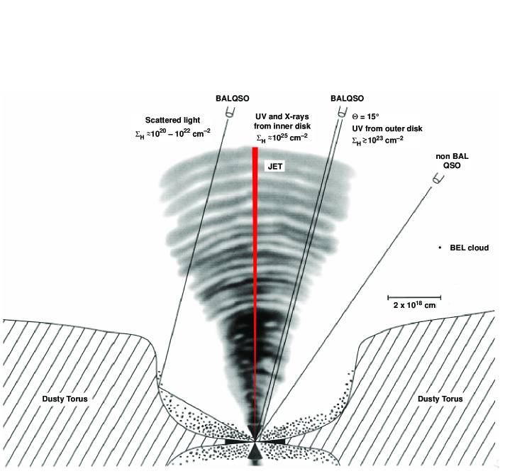
Figure 1: The bipolar wind model of Punsly (1999a, b). The gray clouds of the BAL wind has an opening angle of $\sim 25^{\circ}$ - $30^{\circ}$. Nested inside is a relativistic jet (in red). The highest BAL wind densities are near the polar axis. Thus, lines of sight near the polar axis, have the maximum attenuation of X-ray and ionizing UV radiation from the accretion flow. This implies that lines of sight close to the polar axis are more likely to represent LoBALQSOs.

References

- Antonucci (1993) Antonucci, R.J. 1993, Annu. Rev. Astron. Astrophys. 31 473
- Arnaud (1996) Arnaud, K.A., 1996, Astronomical Data Analysis Software and Systems V, eds. Jacoby G. and Barnes J., ASP Conf. Series volume 101, p17
- Becker et al. (1997) Becker, R.H., Gregg, M.D., Hook, I.M., McMahon, R.G., White, R.L., & Helfand, D.J. 1997, ApJL textbf479 93
- Condon (1997) Condon, J.J. 1997, PASP 109 1149
- Condon et al (1998) Condon, J.J. et al 1998, AJ 115 1693
- De Villiers et al (2005) De Villiers, J-P., Hawley, J., Krolik, J.,Hirose, S. 2005, ApJ 620 878
- Gunn (1978) Gunn, J. 1978 in Observational Cosmology, Eight Advance Course, Swiss Society of Astronomy and Astrophysics, p. 26 eds A. Maeder, L. Martinet and G. Tammann (Geneva Observatory: Sauverny Switzerland)
- Hawley and Krolik (2006) Hawley, J., Krolik, K. 2006, ApJ 641 103
- Hewett and Foltz (2003) Hewett, P. and Foltz, C., 2003 AJ 125 1784
- Kellermann & Pauliny-Toth (1969) Kellermann, K. I., & Pauliny-Toth, I. I. K. 1969 ApJ, 155, L71
- Lind and Blandford (1985) Lind, K., Blandford, R. 1985, ApJ 295 358 345
- Murray et al (1995) Murray, N. et al 1995, ApJ 451 498
- Pen (1999) Pen, U.-L. 1999, ApJS 120 49
- Punsly (1999a) Punsly, B. 1999, ApJ 527 609
- Punsly (1999b) Punsly, B. 1999, ApJ 527 624
- Punsly and Lipari (2005) Punsly, B. 2005, ApJL 623 101
- Reichard et al. (2003) Reichard, T.A., et al. 2003, AJ 126 2594
- Schlegel et al. (1998) Schlegel, D. J., Finkbeiner, D. P. & Davis, M. 1998, ApJ 500 525
- Weymann et al. (1991) Weymann, R.J., Morris, S.L., Foltz, C.B., Hewett, P.C. 1991, ApJ 373, 23
- Weymann (1997) Weymann, R. 1997 in ASP Conf. Ser. 128, Mass Ejection from Active Nuclei ed, N.Arav, I. Shlosman and R.J. Weymann (San Francisco: ASP) 3
- Zhou et al (2006) Zhou, H. et al 2006 ApJ 639 716