Clump Lifetimes and the Initial Mass Function

Abstract

Recent studies of dense clumps/cores in a number of regions of low-mass star formation have shown that the mass distribution of these clumps closely resembles the initial mass function (IMF) of field stars. One possible interpretation of these observations is that we are witnessing the fragmentation of the clouds into the IMF, and the observed clumps are bound pre-stellar cores. In this paper, we highlight a potential difficulty in this interpretation, namely that clumps of varying mass are likely to have systematically varying lifetimes. This ‘timescale’ problem can effectively destroy the similarity bewteen the clump and stellar mass functions, such that a stellar-like clump mass function (CMF) results in a much steeper stellar IMF. We also discuss some ways in which this problem may be avoided.

1 Introduction

One of the major goals in studying star formation is to understand what determines the observed distribution of stellar masses, the initial mass function (IMF). There have been a number of ideas to explain the origins of the IMF including fragmentation, accretion, magnetic fields and stellar feedback (for a list of theories, see references within Shu, Adams & Lizano 1987; Mac Low & Klessen 2004; Bonnell, Larson & Zinnecker 2006). One of the most intriguing developments has been the recent finding that the mass distribution of prestellar cores, those that have not yet, but appear to be on the verge of forming stars, is similar to the stellar IMF (Motte, André & Neri 1998; Testi & Sargent 1998;Johnstone et al. 2000; Johnstone et al. 2001, 2006; Nutter & Ward-Thompson 2006). This has led to the suggestion that fragmentation during the pre-stellar regime leads directly to the stellar IMF. In such a cloud fragmentation picture, the IMF is essentially primordial, since the clump/core masses are presumed to provide the main gas reservoir for each forming system. Furthermore, models of turbulent fragmentation may be able to explain this distribution of clump masses lending additional weight to this scenario (Fleck, 1982; Hunter & Fleck, 1982; Elmegreen, 1993; Padoan, 1995; Padoan, Nordlund & Jones, 1997; Myers, 2000; Klessen, 2001; Padoan & Nordlund, 2002).

In this paper, we highlight a problem in interpreting the observed clump mass distribution as a population of bound, prestellar, cores. We show that such an interpretation would suggest a final stellar IMF which is significantly steeper than the observed mass function. In Section 2 we briefly discuss the observational studies that have examined the clump mass distributions in the nearby star forming regions. Section 3 contains our description of the timescale problem that one encounters when assuming that these clumps are to be the progenitors of individual stars or systems, and we extend this discussion to include significant fragmentation in Section 4. In Section 5 we discuss ways in which the timescale problem can be avoided and we summurise the paper in Section 6. In this paper, we will use the term ‘clump’ to refer to any density enhancement, and ‘core’ or ‘prestellar’ core to refer to those clumps which are going to form stars. We also assume in this paper that the clumps have a density contrast with respect to the ambient cloud such that they are gravitationally decoupled from their surroundings.

2 Clump/Core Observations in Low Mass Star Forming Regions

The first large study of clump masses was published by Motte et al. (1998), for a population of submillimetre cores in $\rho$ Oph. Using data obtained with IRAM, they discovered a total of 58 starless clumps, ranging in mass from 0.05 $\mathrm{M_{\odot}}$ to $\sim 3$ $\mathrm{M_{\odot}}$. The clump mass function (CMF) was shown to be similar to that of the stellar IMF, with power law fit $dn/dm\propto m^{-\alpha}$ following $\alpha=2.5$ above $\sim 0.5$ $\mathrm{M_{\odot}}$ and $\alpha=1.5$ below. Testi & Sargent (1998) confirmed that clumps in Serpens also have a similar mass distribution, taken with the OVRO millimeter-wave array, with their clumps following $\alpha=2.1$ between $\sim 0.6$ $\mathrm{M_{\odot}}$ and $\sim 20$ $\mathrm{M_{\odot}}$ (although some potential caveats with this method have been discussed by Ossenkopf et al. 2001).

Further studies by Johnstone and colleagues of clump properties have been conducted with SCUBA on the JCMT, focusing on $\rho$ Oph (Johnstone et al., 2000), the Orion B North region (Johnstone et al., 2001) and the Orion B south region (Johnstone et al., 2006). The 55 clumps from the $\rho$ Oph study were found to cover a slighly larger range than the Motte et al. (1998) study, going from 0.02 $\mathrm{M_{\odot}}$ to 6.3 $\mathrm{M_{\odot}}$. The mass spectrum was however very similar, with $\alpha=1.5$ below 0.6 $\mathrm{M_{\odot}}$ and $\alpha=2.5$ above, despite differences in both the observational methods and the clump finding techniques used. While observations of clumps in Orion B North yield similar results to those in Serpens and $\rho$ Oph, there does appear to be a distinct difference in the clump properties in Orion B South. The 57 identified cores in the Johnstone et al. (2006) study span a mass range from $\sim 0.4$ $\mathrm{M_{\odot}}$ to $\sim 28$ $\mathrm{M_{\odot}}$ but have a turnover from $\alpha=2.5$ to $\alpha\sim 1.5$ at somewhere between 3 - 10 $\mathrm{M_{\odot}}$, clearly a much higher turnover mass than that found in the other regions. Nutter & Ward-Thompson (2006) have taken this further, using SCUBA archive data on Orion, and find that this higher turnover is true for the region in general. A simlar result was found in the Pipe nebula (see Lada, Alves, Lombardi & Lada 2006), using extinction mapping. One can find more complete discussions of the properties of clumps, or ‘cores’, in the reviews of Di Francesco et al. (2007) and Ward-Thompson et al. (2007).

An exciting interpretation of these observations is that we are witnessing the direct formation of the IMF via fragmentation of the parent cloud. This suggests that there could be a mapping between the observed clumps and the final IMF, with the clumps providing the primary reservior of material for each stars or sytems that form within. Clearly this is an enticing picture, since it implies that one may be able to directly study the origin of the IMF, simply by examining the observable features of the gas. Also, the fact that clumps extend smoothly down past the hydrogen burning limit may then suggest that brown dwarfs form as part of the same process as general star formation (Padoan & Nordlund, 2004). Greaves, Holland & Pound (2003) have even discovered a potential preplanetary clump, which may suggest that this cloud fragmentation process can extend down into the planet mass regime.

However, the evidence that these clumps are the direct origin of the stellar IMF is by no means conclusive. In particular, Johnstone and collaborators (Johnstone et al., 2000; Johnstone et al., 2001, 2006) demonstate that the clumps in their studies are more consistent with stable Bonner-Ebert spheres, and are thus unlikely to be in a state of active star formation. This appears to be the case for all the regions they have studied, including $\rho$ Oph, in which Motte et al. (1998) claim that the majority of clumps are bound. Until recently, most of studies have little, or no, line-width information and are thus unable to accurately determine the internal thermal and kinetic energies of the clumps. Some work has been done for $\rho$ Oph (Belloche, André & Motte, 2001; André, Belloche & Peretto, 2007) and NGC 2068 in the Orion B cloud (André, private communication), which shows that the velocities are low in these regions, suggesting that the contribution to support from internal rotation, and/or turbulence, may be small and so the clumps are bound. These detailed molecular line surveys will we be able to address the concerns that we raise in this paper.

Figure 1: We plot here the range in free-fall times, $t_{ff}$, for a simple IMF, assuming each object in the IMF originates from a clump which has one Jeans mass. The free-fall times are calculated from the Jeans density using a gas temperature of 10 K and a mean molecular weight of $\mu=2.46$.

3 The timescale for fragmentation

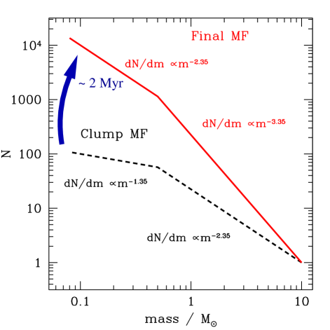
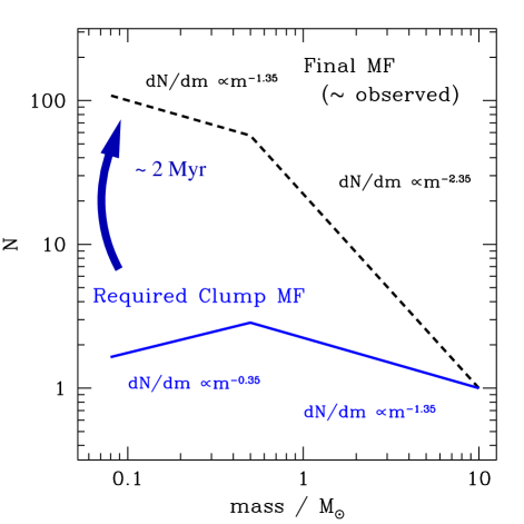
Figure 2: In this figure, we demonstrate what happens when a clump population is permitted to be constantly replenished and for each clump to collapse to form 1 star on its free-fall time (so assuming that each clump has only 1 Jeans mass). The free-fall time for each clump is the same as those given in Figure 1. and the time over which the clump population is evolved is just that for the most massive clump present to collapse, which for a 10 $\mathrm{M_{\odot}}$ star is $t_{ff}(10~{}M_{\odot})\sim$ 2 Myrs. In the left-hand plot, we start with a clump mass population that is very similar to the IMF, which is represented here by the dashed line. The solid line shows the resulting mass spectrum of protostars, after 2 Myrs, taking our three assumptions above. In the right hand plot we show, with the solid line, the clump mass spectrum required to produce a population of protostars which is roughly the same as the stellar IMF. See Section 3 for a discussion of these graphs.

The purpose of this paper is to demonstrate that mapping the observed clump mass function onto the stellar IMF is not straightforward. The problem lies in the fact that clumps of different mass will most likely evolve on different timescales. If one denotes the evolution time of a clump by $t_{evol}$, then the final IMF, $f_{IMF}(m)$, is related to the CMF, $f_{CMF}(m)$, by,

$$f_{IMF}(m)\approx\frac{f_{CMF}(m)~{}\tau_{CMF}}{t_{evol}(m)}$$ (1)

where $m$ denotes the mass of the objects in each case, and $\tau_{CMF}$ is the timescale over which the CMF exists (and we suggest below that this is typically longer than $t_{evol}(m)$, for most $m$). If the evolution timescale for the clump is dependent on its mass, then any power law form that is taken for the CMF will differ from the form of the IMF.

In this section, we will illustrate this problem using some simple Jeans mass and timescale arguments. For the timescale, in the following discussion, we will use the free-fall time, $t_{ff}$, since we are discussing the idea that these clumps are the bound progenitors of young, protostellar, systems.

If each clump is to collapse to form a star, or small $N$ system, then it must have at least one Jeans mass by definition (Jeans, 1902). In its simplest form, the Jeans mass can be thought of as the critical mass at which the (negative) gravitiational energy exceeds the internal energy. For a uniform density sphere, this corresponds to a critical mass,

$$m_{J}=\left[\frac{4\pi\rho}{3}\right]^{-1/2}\left[\frac{5}{2}\frac{kT}{G\mu}\right]^{3/2},$$ (2)

where $\rho$ is the density, $T$ is the temperature, $\mu$ is the mean molecular weight, and $k$ and $G$ are the Boltzmann and gravitational constants, respectively. For simplicity, we will first assume that each clump has one Jeans mass, although we will relax this later on. Assuming the temperature in the region is roughly constant, the clump mass then needs to vary with the clump density in the same way as the Jeans mass,

$$m\propto\rho^{-1/2},$$ (3)

such that low mass clumps need to have a higher density than their high mass companions. Note that a single density is sufficient to describe the clump, since gravity only responds to the volume averaged density (for example, the critical Bonnor-Ebert mass is only a factor of $\sim 2$ smaller than the Jeans mass, despite the density profile in the Bonnor-Ebert sphere). In the absence of any other form of support, and assuming no further external compression, the core will collapse on its free-fall time, $t_{ff}$, which is again dependent on the volume averaged density,

$$t_{ff}\propto\rho^{-1/2}.$$ (4)

Ward-Thompson et al. (2007) have also shown that there exists a systemic trend in clump lifetime with density, and at the densities we consider here, this is of the order of the free-fall time. If the clumps are to be marginally bound, then their collapse timescale should be a function of their mass,

$$t_{collapse}\propto m_{clump}.$$ (5)

Even in cases where magnetic fields and ambipolar diffusion are significant, once the clump becomes bound (supercritical), it collapses on a timescale which is proportional to the free-fall time (Tassis & Mouschovias, 2004). So if one assumes that all the clumps are involved in creating stars, higher mass clumps should take longer to form their protostars than lower mass clumps. Given the two orders of magnitude in mass that is present in the IMF, one then requires a population of clumps which collapse with a similar range in timescales. The clump mass function can then be converted to a distribution of collapse timescales, which we plot in Figure 1. In making this figure, we have used the Jeans mass, given by equation 2 and the free-fall time, given by

$$t_{ff}=\left(\frac{3\pi}{32G\rho}\right)^{1/2},$$ (6)

where $G$ is the standard gravitational constant. In calculating the density from the Jeans mass, we assume a gas temperature of 10K and a mean molecular weight of 2.46.

There are two immediate questions. First, assuming that these clumps are the progenitors of future stellar systems, and noting that they should have different evolutionary timescales, why do we see all the clumps at the same time? Second, why do we also see this same distribution in each of the nearby star-forming regions?

The fact that (roughly) the same clump mass distribution is seen in so many regions of active star formation suggests that such a clump population is constant in time, since all the regions have different ages. Otherwise we would have to assume that we have caught these regions at a very special time in their evolution, and that that special time is right now. This is made more unlikely by the fact that both the dynamical timescale (or crossing time) and the free-fall time of the low mass clumps are remarkably short (as little as $10^{4}$ years) in comparison to the age estimates of local star-forming regions. Therefore ‘now’ would have to be within $10^{4}$ years of each region’s special evolutionary phase. It thus seems reasonable to assume that the observed form of the clump mass function is not a brief phase in a star-forming region’s evolution. It should also be noted here that the clump mass function is also expected to be time-independent in an environment which is dominated by driven turbulence (for example, see Ballesteros-Paredes et al. 2006; Padoan et al. 2007).

The mapping between the clumps and stars/systems can only make sense if what we observe as the clump mass distribution is a uniquely occurring population of pre-stellar cores, and we show here why this is the case. If the clump population is constantly collapsing to form stars on local free-fall times, and if the clumps are constantly being replenished, then one would have a mass function of stars that has many more low mass objects than what is observed for the IMF. This is because low mass clumps have shorter lifetimes than their higher mass siblings, and they are being constantly replenished such that the pre-collapse clump population remains constant in time.

We can demonstrate this by evolving a simple mass function for the time that the highest mass clump takes to collapse, and making the following assumptions:

1. The clump mass distribution is constant in time (always replenished).

2. The clumps each have roughly 1 Jeans mass.

3. The clumps collapse on the corresponding free-fall timescale.

For illustration, we will assume a clump IMF of

$$\begin{array}[]{ll}dN(m)\propto m^{-1.35}dm&0.08<m/M_{\odot}<0.5\\ &\\ dN(m)\propto m^{-2.35}dm&m/M_{\odot}>0.5,\\ \end{array}$$ (7)

which is similar to those quoted in Section 2 which have been observed in active regions of nearby star formation. Note here that our high mass power law is roughly Salpeter (Salpeter, 1955), but neither the exact form of the mass function, nor the lowest mass bin, are important to the following discussion.

In Figure 2, we plot the evolution of two clump mass funtions. The left hand plot shows how a clump population, that is similar to the stellar IMF, evolves to form a population of protostars, based on the three assumptions stated above. Since the highest mass clump in the mass distribution has 10 $\mathrm{M_{\odot}}$, we evolve the clump mass spectra until this clump has collapsed, that is, for a time of roughly 2 Myrs. In Expression 5, we see that there exists a linear relationship between the timescale for collapse and the mass of the clump. This means that ten 1 $\mathrm{M_{\odot}}$ stars can form in the same period as one 10 $\mathrm{M_{\odot}}$ star. Such a linear timescale-mass relationship then results in an increase in the power of the final mass function, such that a clump mass distribution described by Expression 7 results in a much steeper stellar IMF like,

$$\begin{array}[]{ll}dN(m)\propto m^{-2.35}dm&0.08<m/M_{\odot}<0.5\\ &\\ dN(m)\propto m^{-3.35}dm&m/M_{\odot}>0.5.\\ \end{array}$$ (8)

This is clearly much steeper than the stellar IMF, and not consistent with the clump IMF that we start with.

Using this result, it is then possible to work backwards, and determine what clump mass function one should observe if such a process is to generate the IMF. This is done by simply by subtracting 1 from the power in the mass function, giving,

$$\begin{array}[]{ll}dN(m)\propto m^{-0.35}dm&0.08<m/M_{\odot}<0.5\\ &\\ dN(m)\propto m^{-1.35}dm&m/M_{\odot}>0.5.\\ \end{array}$$ (9)

This is shown graphically in the right hand plot in Figure 2. It is clear for the figure that the required clump mass function is much shallower than those quoted in Section 2, for the simple picture we have outlined here. In fact, the required clump mass function is much more similar to that commonly quoted for the internal structure of molecular clouds in general, which is observed to follow a $\sim 1.5$ power (Loren, 1989; Stutzki & Guesten, 1990; Blitz, 1991; Williams, de Geus & Blitz, 1994).

4 Clumps with Multiple Jeans Masses

In the previous section we showed how a distribution of clump masses would evolve into a stellar population, assuming that the clump distribution was constant in time and that each clump had 1 thermal Jeans mass. In such conditions, each clump would form roughly 1 star, resulting in a strong mapping between the clump mass function and the IMF (as has been suggested by Shu et al. 2004). This is an extreme picture. Current observations show that the multiplicity of young stellar objects is higher than in the field-star population, and that these protostellar systems exist on scales smaller, or similar to, the average clump size in the region (Duchêne et al., 2004; Correia et al., 2006). Indeed, there is now mounting evidence that the observed clump mass distribution should be the origin of small $N$ systems rather than single stars (for example, see André et al. 2000; Goodwin et al. 2004a, b). For the clumps to fragment, it is likely that they will then need to have serveral Jeans masses in their initial configuration (Tohline, 1980; Larson, 1985; Shu et al., 1987; Bastien et al., 1991; Burkert & Bodenheimer, 1993; Bonnell, 1999; Tsuribe & Inutsuka, 1999; Tohline, 2002; Sterzik et al., 2003; Goodwin et al., 2004a, b). One therefore needs to examine the evolution of a clump mass distribution in which the members have a range of Jeans masses.

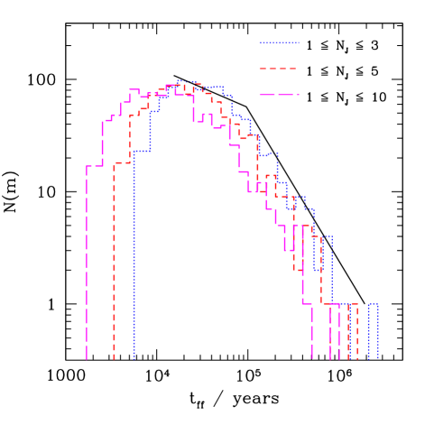
Figure 3: We plot here the range in free-fall times, $t_{ff}$, for a simple clump mass function (same as in figure 1), but this time we assume that the clumps have a random number of Jeans masses, within some predefined range. The assumption of 1 Jeans mass per clump is represented by the solid mass function. The free-fall times are calculated from the Jeans density using a gas temperature of 10 K and a mean molecular weight of $\mu=2.46$.

In Figure 3 we plot the timescale distribution for a clump distribution which covers the same mass range as is given in Expression 7. Assuming that each clump has one Jeans mass, we get the analytic solution discussed above. This is shown in Figure 3 as the solid (black) line. Note that this has the exactly the same form as that plotted in Figure 1. We also plot 3 other distributions in Figure 3, in which we assume each clump can have between 1 and $N_{J}$ Jeans masses, with $N_{J}=$ 3, 5 and 10. For each clump, $N_{J}$ is chosen randomly from a uniform distribution in the permitted range. A clump with mass $m_{clump}$ will then have an associated Jeans mass of $m_{J}=m_{clump}/N_{J}$. If the temperature remains constant, the density of the clump is then given by the Jeans mass relation (2), which is turn translates into a free-fall time, given by Equation 6. It is the distribution of these new timescale that is plotted in Figure 3.

The important feature to note from Figure 3 is that the distribution of collapse timescales becomes wider as the clumps increase their potential to fragment. This means that clumps which are capable of forming small $N$ systems, such as binaries or triples, are also susceptable to the timescale problem that we discuss in Section 3.

5 Avoiding the timescale problem

The most obvious way the clump population could avoid the timescale problem is for all the clumps to have roughly the same density, since then their free-fall timescales would be centred around a regional value.

This is the route Padoan & Nordlund (2002) follow. They describe how an IMF-like distribution of Jeans unstable clumps can be formed naturally via the supersonic turbulence in molecular clouds. They predict that the shock jump-conditions in a molecular gas give rise to a clump population which is characterised by a roughly uniform density (Note that $\rho_{clump}\propto m_{clump}^{1/6}$ in their model). The higher-mass clumps are, most likely, Jeans unstable, since the Jeans mass is lower for these clumps. However as one moves to progressively lower-mass clumps, this is not the case. One must then look to what fraction of the total clumps have a density higher than that predicted from the jump-conditions, and Padoan & Nordlund (2002) make use of the density PDF to estimate this bound fraction of clumps. As a result, the high-mass clumps in the Salpeter section are characterised by single density, and so the largest have many Jeans masses, while the lower-mass clumps follow the same density scaling law as we describe above. The lower-mass clumps (to the left of the turnover point) are therefore susceptable to the timescale problem that we outline in this paper. We therefore expect that the Padoan & Nordlund (2002) CMF would result in more low-mass stars than is seen in the stellar IMF.

While a single common clump density does get around the timescale problem, it is unlikely that the CMF will be the dominant factor which controls the IMF under these conditions. This is due to the process of competitive accretion (Larson 1978; Zinnecker 1982; Bonnell et al. 1997; Bonnell et al. 2001, 2001; Klessen 2001; Bonnell, Larson & Zinnecker 2007; although see also the debate between Krumholz, McKee & Klein 2005 and Bonnell & Bate 2006), which will result in the clumps competing for the available mass, including the mass which currently ‘belongs’ to other clumps. A single density also means a single Jeans mass (assuming a roughly constant temperature), and so clumps masses progressively larger than this Jeans mass become increasingly more unstable to fragmentation (Burkert & Bodenheimer, 1993; Tsuribe & Inutsuka, 1999; Delgado-Donate et al., 2004; Goodwin et al., 2004a, b). This results in small $N$ systems, in which competitive accretion will also be an important process.

Thus it seems that while the timescale problem can be avoided if the clumps are characterised by a single density, competetive accretion would most likely dominate the final IMF. For a CMF to be the progenitor of the IMF, the majority of the objects must be bound, have a common density and be able to resist both high levels of sub-fragmentation and competitive accretion. Note that recent results show that even weak magnetic fields may be able to inhibit fragmentation to some extent (Hosking & Whitworth, 2004; Ziegler, 2005; Fromang et al., 2006), so the fragmentation issue might still be avoided.

One could perhaps argue that the discussion in Section 3 above is too simplistic, since we ignored any non-thermal forms of support, such as rotation, turbulence and magnetic fields, all of which could potentially alter the timescale for the collapse of a clump. However from numerical studies it is typically found that rotational or turbulent support does not substantially alter the collapse timescale (for example, see Tsuribe & Inutsuka 1999; Banerjee et al. 2006). The reason is simply that such forms of support are typically non-isotropic, allowing collapse to occur along favorable directions, with a timescale given by (roughly) the free-fall time. A similar argument holds for magnetic support (Heitsch et al., 2001).

In a magnetically dominated gas it is theoretically possible to remove the mass dependency of the clump collapse timescale, providing both the local mass-to-flux ratio and ionisation fractions are favourably balanced (Tassis & Mouschovias, 2004). However, at present, there is no compelling reason why such a delicate balance should exist. One can construct a similar situation by varying the temperature in the clumps. In such a case, the Jeans mass variation from clump to clump would be controlled primarily by the temperature, with the density being constant ($m_{J}\propto\rho^{-1/2}T^{3/2}$). However this would still require a temperature range from around 2 K to 45 K for clumps in the range 0.1 $\mathrm{M_{\odot}}$ to 10 $\mathrm{M_{\odot}}$, respectively. Line-width observations suggest that such a wide range of temperatures is not to be expected, and indeed clump mass estimates from sub-mm observations tend to assume a single temperature for a star-forming ‘core’ in the range 10 - 20 K.

The ‘hierarchical’ fragmentation picture (Hoyle, 1953) would also avoid the timescale problem, and indeed Larson (1973) suggested that such a process may be able to form a mass function of fragments similar to the IMF. One could perhaps argue that the regions in which the clump masses are observed to be larger (Johnstone et al., 2006; Lada et al., 2006; Nutter & Ward-Thompson, 2006) are just in an earlier stage of the hierarchical collapse process. However as Larson (1973) pointed out, one needs some way of preventing the fragments from merging and in fact no simulation to date has shown signs of hierarchical fragmentation, as it is described in the models (Larson, 2007). The main problem is that it is not possible for density fluctuations to grow faster than the ambient collapse, unless these fluctuations have Jeans mass to start with (Tohline, 1980), which results in initial conditions that have many Jeans masses. These are exactly the conditions required for the competitive accretion process (Bonnell & Bate, 2006).

The timescale problem is avoided entirely if the clump mass population plays no part in shaping the IMF, and the similarities between the two mass function is just a coincidence. Recent numerical simulations have suggested that this might be the case. In both studies of driven (Klessen et al., 2000; Klessen, 2001) and freely decaying turbulence (Clark & Bonnell, 2005), the vast majority of clumps are unbound, with only the more massive of those in the distribution gaining the neccessary conditions to form stars. Not only do the lower mass clumps have kinetic energies in excess of their gravitational potential energy, but they very seldom possess a Jeans mass (that is, their thermal energy is larger that that from self-gravity, for example see Klessen et al. 2005). The highest mass objects, forming at the stagnation points of convergent turbulent flows, eventually become completely bound, gain multiple Jeans masses and fragment into small $N$ groups. The IMF in such simulations is largely controlled by the competitve accretion process. The fact that there exists an ever present population of clumps which resembles the IMF is never a problem, since almost all the low mass objects are transient (Klessen, 2001; Tilley & Pudritz, 2004; Clark & Bonnell, 2005; Vázquez-Semadeni et al., 2006; Clark & Bonnell, 2006).

Note that the timescale problem that we highlight here applies to all theories which directly try to produce an IMF-style distribution of fragments, with exception of the ‘hierarchical’ model (Hoyle, 1953; Larson, 1973), although as we note above, this contains its own problems. This is also true (in varying degrees) of the ‘turbulent fragmentation’ theories (Fleck, 1982; Hunter & Fleck, 1982; Elmegreen, 1993; Padoan, 1995; Padoan et al., 1997; Myers, 2000; Padoan & Nordlund, 2002), and Elmegreen (1993) raised a similar point to the one we make here in his study,

6 Conclusions

We have presented a potential problem with interpreting the observed clump mass function (CMF) as the direct origin of the stellar (or system) IMF. If each clump is assumed to be a star-forming core, then it must have at least one Jeans mass. If the clumps have a comparable number of Jeans masses, then the low-mass clumps must have much higher densities than the high-mass clumps. This in turn translates into a range of free-fall times which are proportional to clump mass. Thus clumps of different mass are evolving on different timescales. If one then assumes the clump mass function is constant in time, as is suggested by its presence in most of the nearby star forming regions, then the resulting stellar mass function is significantly steeper than the observed IMF (an increase of $+1$ in the power-law fit).

The alternative is that all clumps have the same density, and thus evolve on the same timescale. However this also means that the more massive clumps are perhaps increasingly susceptible to fragmentation and may produce produce systems of lower-mass stars (although see the recent magnetic studies which yield reduced levels of fragmentation: Hosking & Whitworth 2004; Ziegler 2005; Fromang et al. 2006). Attaining higher masses would then necessitate subsequent accretion. Under such conditions we point out that competitive accretion should become an important ingredient in shaping the final IMF (for example, see Bonnell & Bate 2006).

We therefore conclude that the mass function of clumps that directly turns into individual stars and higher-order systems, needs to be either considerably shallower than is inferred for nearby star-forming regions, or needs to avoid sub-fragmentation and competitive accretion.

7 Acknowledgements

The authors would like to thank the LOC responsible for the ‘Early Phase of Star Formation’ meeting held at Ringberg Castle Germany (28th August to 1st September 2006) which provided the final impedous for the completion of this paper. On a more personal level, we would also like to thank Phillipe André, Bruce Elmegreen, Richard Larson, Derek Ward-Thompson, Frank Shu, Robi Banerjee, Ant Whitworth and the anonymous referees for many helpful discussions. PCC acknowledges support from the German Science Foundation (via grant KL1358/5).

References

- André et al. (2007) André P., Belloche A., Peretto N., 2007, in prep
- André et al. (2000) André P., Motte F., Neri R., 2000, in Mangum J. G., Radford S. J. E., eds, ASP Conf. Ser. 217: Imaging at Radio through Submillimeter Wavelengths IRAM 30m Continuum Surveys of Star-Forming Regions. p. 152
- Ballesteros-Paredes et al. (2006) Ballesteros-Paredes J., Gazol A., Kim J., Klessen R. S., Jappsen A.-K., Tejero E., 2006, ApJ, 637, 384
- Banerjee et al. (2006) Banerjee R., Pudritz R. E., Anderson D. W., 2006, MNRAS, p. 1232
- Bastien et al. (1991) Bastien P., Arcoragi J., Benz W., Bonnell I., Martel H., 1991, ApJ, 378, 255
- Belloche et al. (2001) Belloche A., André P., Motte F., 2001, in Montmerle T., André P., eds, ASP Conf. Ser. 243: From Darkness to Light: Origin and Evolution of Young Stellar Clusters Kinematics of Millimeter Prestellar Condensations in the Ophiuchi Protocluster. p. 313
- Blitz (1991) Blitz L., 1991, in NATO ASIC Proc. 342: The Physics of Star Formation and Early Stellar Evolution Star Forming Giant Molecular Clouds. p. 3
- Bonnell (1999) Bonnell I. A., 1999, in NATO ASIC Proc. 540: The Origin of Stars and Planetary Systems Multiple Stellar Systems: From Binaries to Clusters. p. 479
- Bonnell & Bate (2006) Bonnell I. A., Bate M. R., 2006, MNRAS, 370, 488
- Bonnell et al. (1997) Bonnell I. A., Bate M. R., Clarke C. J., Pringle J. E., 1997, MNRAS, 285, 201
- Bonnell et al. (2001) Bonnell I. A., Bate M. R., Clarke C. J., Pringle J. E., 2001, MNRAS, 323, 785
- Bonnell et al. (2001) Bonnell I. A., Clarke C. J., Bate M. R., Pringle J. E., 2001, MNRAS, 324, 573
- Bonnell et al. (2006) Bonnell I. A., Larson R. B., Zinnecker H., 2006, in Protostars and Planets V, in press The Origin of the Initial Mass Function
- Bonnell et al. (2007) Bonnell I. A., Larson R. B., Zinnecker H., 2007, in Reipurth B., Jewitt D., Keil K., eds, Protostars and Planets V The Origin of the Initial Mass Function. pp 149–164
- Burkert & Bodenheimer (1993) Burkert A., Bodenheimer P., 1993, MNRAS, 264, 798
- Clark & Bonnell (2005) Clark P. C., Bonnell I. A., 2005, MNRAS, 361, 2
- Clark & Bonnell (2006) Clark P. C., Bonnell I. A., 2006, MNRAS, 368, 1787
- Correia et al. (2006) Correia S., Zinnecker H., Ratzka T., Sterzik M. F., 2006, A&A, 459, 909
- Delgado-Donate et al. (2004) Delgado-Donate E. J., Clarke C. J., Bate M. R., 2004, MNRAS, 347, 759
- Di Francesco et al. (2007) Di Francesco J., Evans II N. J., Caselli P., Myers P. C., Shirley Y., Aikawa Y., Tafalla M., 2007, in Reipurth B., Jewitt D., Keil K., eds, Protostars and Planets V An Observational Perspective of Low-Mass Dense Cores I: Internal Physical and Chemical Properties. pp 17–32
- Duchêne et al. (2004) Duchêne G., Bouvier J., Bontemps S., André P., Motte F., 2004, A&A, 427, 651
- Elmegreen (1993) Elmegreen B. G., 1993, ApJL, 419, L29
- Fleck (1982) Fleck R. C., 1982, MNRAS, 201, 551
- Fromang et al. (2006) Fromang S., Hennebelle P., Teyssier R., 2006, A&A, 457, 371
- Goodwin et al. (2004a) Goodwin S. P., Whitworth A. P., Ward-Thompson D., 2004a, A&A, 414, 633
- Goodwin et al. (2004b) Goodwin S. P., Whitworth A. P., Ward-Thompson D., 2004b, A&A, 423, 169
- Greaves et al. (2003) Greaves J. S., Holland W. S., Pound M. W., 2003, MNRAS, 346, 441
- Heitsch et al. (2001) Heitsch F., Mac Low M.-M., Klessen R. S., 2001, ApJ, 547, 280
- Hosking & Whitworth (2004) Hosking J. G., Whitworth A. P., 2004, MNRAS, 347, 1001
- Hoyle (1953) Hoyle F., 1953, ApJ, 118, 513
- Hunter & Fleck (1982) Hunter J. H., Fleck R. C., 1982, ApJ, 256, 505
- Jeans (1902) Jeans J. H., 1902, Phil. Trans. Roy. Soc., 199, 1
- Johnstone et al. (2001) Johnstone D., Fich M., Mitchell G. F., Moriarty-Schieven G., 2001, ApJ, 559, 307
- Johnstone et al. (2006) Johnstone D., Matthews H., Mitchell G. F., 2006, ApJ, 639, 259
- Johnstone et al. (2000) Johnstone D., Wilson C. D., Moriarty-Schieven G., Joncas G., Smith G., Gregersen E., Fich M., 2000, ApJ, 545, 327
- Klessen (2001) Klessen R. S., 2001, ApJ, 556, 837
- Klessen et al. (2005) Klessen R. S., Ballesteros-Paredes J., Vázquez-Semadeni E., Durán-Rojas C., 2005, ApJ, 620, 786
- Klessen et al. (2000) Klessen R. S., Heitsch F., Mac Low M., 2000, ApJ, 535, 887
- Krumholz et al. (2005) Krumholz M. R., McKee C. F., Klein R. I., 2005, Nature, 438, 332
- Lada et al. (2006) Lada C. L., Alves J. F., Lombardi M., Lada E. A., 2006, in Protostars and Planets V, in press Near-Infrared Extinction and the Structure and Nature of Molecular Clouds
- Larson (1973) Larson R. B., 1973, MNRAS, 161, 133
- Larson (1978) Larson R. B., 1978, MNRAS, 184, 69
- Larson (1985) Larson R. B., 1985, MNRAS, 214, 379
- Larson (2007) Larson R. B., 2007, ArXiv Astrophysics e-prints
- Loren (1989) Loren R. B., 1989, ApJ, 338, 902
- Mac Low & Klessen (2004) Mac Low M., Klessen R. S., 2004, Reviews of Modern Physics, 76, 125
- Motte et al. (1998) Motte F., André P., Neri R., 1998, A&A, 336, 150
- Myers (2000) Myers P. C., 2000, ApJL, 530, L119
- Nutter & Ward-Thompson (2006) Nutter D., Ward-Thompson D., 2006, astro-ph/0611164
- Ossenkopf et al. (2001) Ossenkopf V., Klessen R. S., Heitsch F., 2001, A&A, 379, 1005
- Padoan (1995) Padoan P., 1995, MNRAS, 277, 377
- Padoan & Nordlund (2002) Padoan P., Nordlund Å., 2002, ApJ, 576, 870
- Padoan & Nordlund (2004) Padoan P., Nordlund Å., 2004, ApJ, 617, 559
- Padoan et al. (1997) Padoan P., Nordlund Å., Jones B. J. T., 1997, MNRAS, 288, 145
- Padoan et al. (2007) Padoan P., Nordlund Å., Kritsuk A. G., Norman M. L., Li P. S., 2007, ArXiv Astrophysics e-prints
- Salpeter (1955) Salpeter E. E., 1955, ApJ, 121, 161
- Shu et al. (1987) Shu F. H., Adams F. C., Lizano S., 1987, ARA&A, 25, 23
- Shu et al. (2004) Shu F. H., Li Z.-Y., Allen A., 2004, in Johnstone D., Adams F. C., Lin D. N. C., Neufeeld D. A., Ostriker E. C., eds, ASP Conf. Ser. 323: Star Formation in the Interstellar Medium: In Honor of David Hollenbach The Stellar Initial Mass Function. pp 37–+
- Sterzik et al. (2003) Sterzik M. F., Durisen R. H., Zinnecker H., 2003, A&A, 411, 91
- Stutzki & Guesten (1990) Stutzki J., Guesten R., 1990, ApJ, 356, 513
- Tassis & Mouschovias (2004) Tassis K., Mouschovias T. C., 2004, ApJ, 616, 283
- Testi & Sargent (1998) Testi L., Sargent A. I., 1998, ApJL, 508, L91
- Tilley & Pudritz (2004) Tilley D. A., Pudritz R. E., 2004, MNRAS, 353, 769
- Tohline (1980) Tohline J. E., 1980, ApJ, 239, 417
- Tohline (2002) Tohline J. E., 2002, ARA&A, 40, 349
- Tsuribe & Inutsuka (1999) Tsuribe T., Inutsuka S., 1999, ApJ, 526, 307
- Vázquez-Semadeni et al. (2006) Vázquez-Semadeni E., Ryu D., Passot T., González R. F., Gazol A., 2006, ApJ, 643, 245