Theory of Two-Photon Interactions with Broadband Down-Converted Light and Entangled Photons

Abstract

When two-photon interactions are induced by down-converted light with a bandwidth that exceeds the pump bandwidth, they can obtain a behavior that is pulse-like temporally, yet spectrally narrow. At low photon fluxes this behavior reflects the time and energy entanglement between the down-converted photons. However, two-photon interactions such as two-photon absorption (TPA) and sum-frequency generation (SFG) can exhibit such a behavior even at high power levels, as long as the final state (i.e. the atomic level in TPA, or the generated light in SFG) is narrowband enough. This behavior does not depend on the squeezing properties of the light, is insensitive to linear losses, and has potential applications. In this paper we describe analytically this behavior for travelling-wave down-conversion with continuous or pulsed pumping, both for high- and low-power regimes. For this we derive a quantum-mechanical expression for the down-converted amplitude generated by an arbitrary pump, and formulate operators that represent various two-photon interactions induced by broadband light. This model is in excellent agreement with experimental results of TPA and SFG with high power down-converted light and with entangled photons [Dayan et al., Phys. Rev. Lett. 93, 023005 (2004), 94, 043602, (2005), Pe’er et al., Phys. Rev. Lett. $\textbf{94},$ 073601 (2005)].

I Introduction

Parametrically down-converted light Giallorenzi and Tang (1968); Byer and Harris (1968); Hong and Mandel (1985); Mandel and Wolf (1995) exhibits correlations between the down-converted modes, and has been a primary source in experimental quantum-optics Mattle et al. (1996); Bouwmeester et al. (1997); Furusawa et al. (1998); Boschi et al. (1998); Jennewein et al. (2000); Naik et al. (2000); Tittel et al. (2000). At low photon-fluxes, these correlations are inherently nonclassical, and are exhibited in the generation of entangled photon-pairs Burnham and Weinberg (1970); Mandel (1982); Kwiat et al. (1993, 1995). Two-photon interactions induced by entangled photons are expected to exhibit nonclassical features, in particular a linear dependence on the intensity Janszky and Yushin (1987); Gea-Banacloche (1989); Javanainen and Gould (1990); Fei et al. (1997); Saleh et al. (1998); Perina et al. (1998); Georgiades et al. (1999), as was observed with two-photon absorption (TPA) Georgiades et al. (1995) and with sum-frequency generation (SFG) Dayan et al. (2005). At higher powers, the correlations between the down-converted modes are better expressed as quadrature correlations. In this regime, the nonclassical nature of the correlations lies in the fact that their precision can exceed the vacuum shot-noise level, a phenomenon that is named squeezing Mollow and Glauber (1967a, b); Mandel (1982); McNeil and Gardiner (1983); Walls (1983); Wu et al. (1986); Slusher et al. (1987); Laurat et al. (2005, 2006); Takeno et al. (2007), and is expected to effect two-photon interactions even at photon-fluxes which exceed the single photon regime Janszky and Yushin (1987); Ficek and Drummond (1991); Gardiner and Parkins (1994); Zhou and Swain (1996); Turchette et al. (1998); Georgiades et al. (1999). However, while squeezing (i.e. the high precision of the correlations) is easily destroyed (for example, by linear losses), the remaining correlations still have a dramatic effect on two-photon interactions. Specifically, when the down-converted bandwidth is significantly larger than the pump bandwidth, the down-converted light can induce two-photon interactions with the same efficiency and sharp temporal behavior as ultrashort pulses, while exhibiting high spectral resolution as that of the narrowband pump Abram et al. (1986); Dayan et al. (2003, 2004); Pe’er et al. (2005). Although at low photon fluxes these properties are a manifestation of the time and energy entanglement between the down-converted photons, at high powers exactly the same properties are exhibited if the final state of the induced two-photon interaction is narrowband enough Dayan et al. (2004). This effect occurs since the narrow bandwidth of the final state ”post-selects” only the contribution of photon pairs that are complementary in energy. Thus, in the high-power regime, these seemingly nonclassical properties are completely described within the classical framework (in fact, they are equivalent to the correlations that exist between the transmitted signal and its key in spread-spectrum communication systems Pe’er et al. (2004)), and do not depend on the squeezing degree of the down-converted light. This equivalence of broadband down-converted light to coherent ultrashort pulses also implies an ability to coherently control and shape the induced two-photon interactions with pulse-shaping techniques, although the down-converted light is neither coherent, nor pulsed. This effect was demonstrated both in high power Dayan et al. (2003, 2004) and with broadband entangled photons Pe’er et al. (2005), in which case it can be viewed as shaping of the second-order correlation function of the entangled photons $\texttt{g}^{2}(\tau)$. The fact that these unique properties can be exhibited at high powers, with no dependence on nonclassical features of the light (such as entanglement or squeezing), makes this phenomena both interesting and applicable Pe’er et al. (2004, 2006).

In this paper we describe analytically this unique behavior of two-photon interactions with broadband down-converted light. First, in section II, we analytically solve the equations of motion for broadband parametric down-conversion with arbitrary pump (continuous or pulsed), obtaining a non-perturbative solution that is valid both for low-power and for high-power down-converted light. The derivation takes into account the specific spectrum of the pump, assuming only that it is significantly narrower than the down-converted spectrum. The solution, namely the annihilation operators for the down-converted fields, is represented as a function of the down-converted spectrum, a property that is typically easy to calculate, estimate or measure.

In section III, we formulate quantum-mechanical operators that can represent multiphoton phenomena, specifically TPA, SFG and coincidence events, induced by any broadband light. By evaluating the expectation value of these operators, using the annihilation operators derived in section II, we obtain in section IV a generic analytic expression for two-photon interactions induced by broadband down-converted light, as a function of the pump spectrum and the down-converted spectrum. In section V we derive specific expressions for TPA, SFG and coincidence events induced by broadband down-converted light, and analyze their temporal and spectral properties. In section VI we give a brief summary of our results and add some concluding remarks.

II Solving the equations of motion for broadband down-conversion with an arbitrary pump

In our derivations we have chosen to use a continuous-variables version of the formalism suggested by Huttner et al. Huttner et al. (1990). This formalism represents the quantum fields in terms of space-dependent spectral mode operators $a(\omega,z)$, instead of time-dependent momentum mode operators $a(k,t)$. The advantage is that unlike momentum modes, temporal modes are unchanged by a dielectric medium, reflecting the physical fact that while the energy density of the fields depends on the medium, the energy flux does not. Accordingly, a temporal periodicity, instead of a spatial periodicity is assumed in the quantization process. We have performed the transition to continuous variables (taking the temporal periodicity to infinity) following the guidelines of the same procedure in momentum and space Blow et al. (1990). Specifically, assuming a single polarization and a single spatial mode we may write:

$$E(t,z)=E^{+}(t,z)+E^{-}(t,z)\ ,\ \$$

$$E^{+}(t,z)=i\int_{0}^{\infty}d\omega\>\sqrt{\frac{\hbar\omega}{4\pi c\varepsilon S}}\ \hat{a}(\omega,z)e^{-i\omega(t-z/c)},\ \ E^{-}(t,z)=\left(E^{+}\left(t,z\right)\right)^{*}$$ (1)

where $S$ is the beam area, $\varepsilon$ is the permittivity, and $\hat{a}^{{\dagger}}(\omega,z),\ \hat{a}(\omega,z)$ are the slowly varying complex amplitudes of the creation and annihilation operators of the electromagnetic field Jeffers and Barnett (1993). A major advantage of this formalism is the relative convenience at which we can define a momentum operator $\hat{G}(z)$ for the electromagnetic field in a dispersive medium, and use it as the generator for space propagation. The equations (and hence the solutions) derived in the following resemble those attained by using the classical Maxwell equations, or by using the Hamiltonian for time propagation and replacing the spatial coordinate $z$ by $tc$ (see, for example, Yariv (1989)); however the derivation presented here is a multimode, continuum-frequency one, enabling us to take into account the specific spectrum of the pump and the fact that each signal mode is coupled by the pump to multiple idler modes, and vice versa.

The momentum operator related to the second-order nonlinear polarization is of the form Shen (1967); Abram (1987); Huttner et al. (1990); Caves and Crouch (1987):

$$\hat{G}^{nl}(z)=\int_{0}^{\infty}d\omega_{p}\int_{0}^{\infty}d\omega\>\hbar\>\beta(\omega_{p},\omega)\left(\hat{a}_{s}(\omega,z)\hat{a}_{i}(\omega_{p}-\omega)\hat{a}_{p}^{{\dagger}}(\omega_{p},z)e^{-i\Delta k(\omega_{p},\omega)z}+H.C.\right)\>,$$

$$\beta(\omega_{p},\omega)=\chi(\omega,\omega_{p})\sqrt{\frac{\hbar\omega_{p}\omega(\omega_{p}-\omega)}{16\pi\varepsilon_{0}c^{3}S\textsl{n}_{p}(\omega_{p})\textsl{n}_{s}(\omega)\textsl{n}_{i}(\omega_{p}-\omega)}}\>,$$ (2)

where the subscripts $s,i,p$ denote the signal, idler and pump modes, respectively, $\textsl{n}_{s,i,p}(\omega_{s,i,p})$ denote the corresponding indices of refraction, and with:

$$\Delta k(\omega_{p},\omega)=k_{p}(\omega_{p})-k_{s}(\omega)-k_{i}(\omega_{p}-\omega)\>.$$ (3)

The primary assumption throughout our calculations is that the down-converted spectrum $\Delta_{\textsc{dc}}$ is considerably broader than the pump bandwidth $\delta_{p}$:

$$\Delta_{\textsc{dc}}\gg\delta_{p}\ ,$$ (4)

where we take $\Delta_{\textsc{dc}}$ to denote the bandwidth of the signal (or the idler) field (note that the signal and the idler have the same bandwidth). Having assumed a narrowband pump, we can safely neglect the dependence of $\chi$ (which is typically real) and $\Delta k$ on $\omega_{p}$, since typically the crystal’s nonlinear properties vary only at much larger scales of frequencies, and write: $\beta(\omega_{p},\omega)=\beta(\omega)$, and $\Delta k(\omega_{p},\omega)=\Delta k(\omega)$. We thus write the equation of motion for $\hat{a_{s}(\omega,z)}$ for undepleted, strong pump, replacing $\hat{a}_{p}(\omega_{p},z)$ with the spectral amplitude of the classical pump field $\textsf{A}_{p}(\omega_{p})$:

$$\frac{\partial\hat{a}_{s}(\omega,z)}{\partial z} = -\frac{i}{\hbar}\big{[}\hat{a}_{s}(\omega,z),\hat{G}^{nl}(z)\big{]}$$ (5)

$$= -i\beta(\omega)e^{-i\Delta k(\omega)z}\int_{0}^{\infty}d\omega_{p}\textsf{A}_{p}(\omega_{p})\>\hat{a}_{i}^{{\dagger}}(\omega_{p}-\omega,z)$$

The same can be formulated for the idler, which leads to:

$$\frac{\partial^{2}\>\hat{a}_{s}(\omega,z)}{\partial z^{2}} = |\beta(\omega)|^{2}\int^{\infty}_{-\infty}d\upsilon\int_{0}^{\infty}d\omega_{p}\>\textsf{A}_{p}(\omega_{p})\>\textsf{A}_{p}^{*}(\omega_{p}+\upsilon)\>\hat{a}_{s}(\omega+\upsilon,z)$$ (6)

$$- \Delta k(\omega)\>\beta(\omega)e^{-i\Delta k(\omega)z}\int_{0}^{\infty}d\omega_{p}\textsf{A}_{p}(\omega_{p})\>\hat{a}_{i}^{{\dagger}}(\omega_{p}-\omega,z)\>,$$

where $\upsilon=\widetilde{\omega}_{P}-\omega_{P}$. For a stationary light field we can write Jeffers et al. (1993):

$$\int_{0}^{\infty}d\omega_{p}\>\textsf{A}_{p}(\omega_{p})\>\textsf{A}_{p}^{*}(\omega_{p}+\upsilon)=2\pi I_{p}\>\delta(\upsilon)$$ (7)

where $I_{p}=\langle\texttt{I}_{p}(t)\rangle=\langle\big{|}A_{p}(t)\big{|}^{2}\rangle$ is the mean power (in units of photon-flux) of the pump field, and so:

$$\int^{\infty}_{-\infty}d\upsilon\int_{0}^{\infty}d\omega_{p}\>\textsf{A}_{p}(\omega_{p})\>\textsf{A}_{p}^{*}(\omega_{p}+\upsilon)\>\hat{a}_{s}(\omega+\upsilon,z)=2\pi I_{p}\>\hat{a}_{s}(\omega,z)\ .$$ (8)

A similar result can be obtained, for non-stationary, pulsed light with a final duration of $\tau_{p}$, by approximating:

$$\int_{0}^{\infty}d\omega_{p}\>\textsf{A}_{p}(\omega_{p})\>\textsf{A}_{p}^{*}(\omega_{p}+\upsilon) \approx \int_{\tau_{p}}\texttt{I}_{p}(t)\>dt\ \ when\ |\upsilon|<\frac{\pi}{\tau_{p}}$$ (9)

$$\approx 0\ \ \ \ \ \ \ \ \ \ otherwise\ .$$

This approximation reflects the fact that the spectral amplitude of a finite signal can be considered roughly constant within spectral slices that are smaller than $2\pi/\tau$, where $\tau$ is the signal’s duration. Accordingly, since (under the condition of Eq. (4)) pulsed down-converted light has a duration which is always equal or shorter than the pump pulse, its spectral components may be regarded as constant over spectral slices that are smaller than $2\pi/\tau_{p}$. For this reason it is safe to approximate:

$$\int^{\infty}_{-\infty}d\upsilon\int_{0}^{\infty}d\omega_{p}\>\textsf{A}_{p}(\omega_{p})\>\textsf{A}_{p}^{*}(\omega_{p}+\upsilon)\>\hat{a}_{s}(\omega+\upsilon,z) \approx \int_{\tau_{p}}\texttt{I}_{p}(t)\>dt\>\beta(\omega)^{2}\int^{\frac{\pi}{\tau_{p}}}_{-\frac{\pi}{\tau_{p}}}d\upsilon\>\hat{a}_{s}(\omega+\upsilon,z)$$ (10)

$$\approx \int_{\tau_{p}}\texttt{I}_{p}(t)\>dt\>\beta(\omega)^{2}\int^{\frac{\pi}{\tau_{p}}}_{-\frac{\pi}{\tau_{p}}}d\upsilon\>\hat{a}_{s}(\omega,z)$$

$$= 2\pi I_{p}\beta(\omega)^{2}\>\hat{a}_{s}(\omega,z)$$

obtaining the same result as with a stationary pump, except for the fact that the averaging $I_{p}=\langle\texttt{I}_{p}(t)\rangle$ is performed over the duration of the pump pulse. Thus, both for stationary and non-stationary pumps, Eq. (6) becomes:

$$\frac{\partial^{2}\>\hat{a}_{s}(\omega,z)}{\partial z^{2}}=2\pi I_{p}\beta(\omega)^{2}\>\hat{a}_{s}(\omega,z)-\Delta k(\omega)\>\beta(\omega)e^{-i\Delta k(\omega)z}\int_{0}^{\infty}d\omega_{p}\textsf{A}_{p}(\omega_{p})\>\hat{a}_{i}^{{\dagger}}(\omega_{p}-\omega,z)\>.$$ (11)

The solution of Eqs. (5) and (11) is:

$$\hat{a}_{s}(\omega,z)\>e^{i\Delta k(\omega)z/2} = \bigg{(}\cosh\big{(}\kappa(\omega)z\big{)}+\frac{i\Delta k(\omega)}{2\kappa(\omega)}\sinh\big{(}\kappa(\omega)z\big{)}\bigg{)}\>\hat{a}_{s}(\omega,0)$$ (12)

$$- \frac{i\beta(\omega)}{\kappa(\omega)}\>\sinh\big{(}\kappa(\omega)z\big{)}\int_{0}^{\infty}d\omega_{P}\>\textsf{A}_{p}(\omega_{p})\>\hat{a}_{i}^{{\dagger}}(\omega_{p}-\omega,0)\>.$$

with:

$$\kappa(\omega)=\sqrt{2\pi I_{p}\beta(\omega)^{2}-\Delta k(\omega)^{2}/4}\ .$$ (13)

The average photon flux spectral density for the signal and the idler fields is therefore Blow et al. (1990):

$$\texttt{n}_{s,i}(\omega,z) = \frac{1}{2\pi}\int_{0}^{\infty}d\omega^{\prime}\big{\langle}vac\big{|}\hat{a}_{s,i}^{{\dagger}}(\omega,z)\hat{a}_{s,i}(\omega^{\prime},z)\big{|}vac\big{\rangle}$$ (14)

$$= \frac{I_{p}\beta(\omega)^{2}}{\kappa(\omega^{2})}\sinh^{2}\big{(}\kappa(\omega)z\big{)}\>.$$

Since the down-converted spectrum can readily be calculated or measured for any specific down-conversion apparatus, we find it convenient to present our following calculations using $\texttt{n}_{s,i}(\omega)$ as given parameters, thus avoiding the issue of evaluating $\chi(\omega)$ and the other elements of $\beta(\omega)$ that determine the down-converted spectrum, and focusing on the behavior of two-photon interactions induced by such a light. Assuming that the down-conversion process occurred along a distance $L$, we denote:

$$n_{s,i}(\omega)=\frac{\kappa(\omega^{2})}{I_{p}\beta(\omega)^{2}}\texttt{n}_{s,i}(\omega,L)=\sinh^{2}\big{(}\kappa(\omega)z\big{)}\ ,$$ (15)

thus obtaining the following simple expression for $\hat{a}_{s,i}(\omega,L)$:

$$\hat{a}_{s,i}(\omega,L)\>e^{i\Delta k(\omega)L/2} = \bigg{(}\sqrt{1+n_{s,i}(\omega)}+\frac{i\Delta k(\omega)}{2\kappa(\omega)}\sqrt{n_{s,i}(\omega)}\>\bigg{)}\>\hat{a}_{s,i}(\omega,0)$$ (16)

$$- \frac{i\beta(\omega)}{\kappa(\omega)}\>\sqrt{n_{s,i}(\omega)}\int_{0}^{\infty}d\omega_{P}\>\textsf{A}_{p}(\omega_{p})\>\hat{a}_{i,s}^{{\dagger}}(\omega_{p}-\omega,0)\>.$$

For good phase-matching conditions (i.e $\Delta k(\omega)\ll\sqrt{I_{p}}\beta(\omega)$), we get $\kappa(\omega)\rightarrow\sqrt{2\pi I_{p}}\beta(\omega)$ and therefore $\Delta k(\omega)/\kappa(\omega)\ll 1$, in which case Eq. (16) can be further simplified to:

$$\hat{a}_{s,i}(\omega,L)\>e^{i\Delta k(\omega)z/2}=\sqrt{1+n_{s,i}(\omega)}\>\hat{a}_{s,i}(\omega,0)-\frac{i}{\sqrt{2\pi I_{p}}}\>\sqrt{n_{s,i}(\omega)}\int_{0}^{\infty}d\omega_{P}\>\textsf{A}_{p}(\omega_{p})\>\hat{a}_{i,s}^{{\dagger}}(\omega_{p}-\omega,0)\>.$$ (17)

with:

$$n_{s,i}(\omega)=2\pi\texttt{n}_{s,i}(\omega,L)\ ,$$ (18)

III Deriving operators for weak two-photon interactions induced by broadband fields

In this section we derive expressions for weak (perturbative) two-photon interactions induced by broadband fields. Limiting ourselves to low efficiencies of interaction, we neglect the depletion of the in-coming fields $a_{1,2}(\omega,z)$ that induce the interaction. Therefore we suppress in the following their dependence on $z$, denoting $a_{1,2}(\omega,z)=a_{1,2}(\omega,0)=a_{1,2}(\omega)$. We begin with specific expressions for SFG and TPA, and then obtain a generic expression which will be used in the following sections.

III.1 SFG

For SFG, we use the nonlinear momentum operator of Eq. (II), replacing $\hat{a}_{p}^{\dagger}$ with the creation operator of the SFG mode $\hat{a}_{\textsc{sfg}}^{\dagger}$:

$$\frac{\partial\hat{a}_{\textsc{sfg}}(\Omega,z)}{\partial z} = -\frac{i}{\hbar}\big{[}\hat{a}_{\textsc{sfg}}(\Omega,z),\hat{G}^{nl}(z)\big{]}$$ (19)

$$= -i\int_{0}^{\infty}d\omega\>\beta(\omega,\Omega)\hat{a}_{1}(\omega)\hat{a}_{2}(\Omega-\omega)e^{-i\Delta k(\omega,\Omega)z}\>,$$

with

$$\Delta k(\Omega,\omega)=k_{\textsc{sfg}}(\Omega)-k_{1}(\omega)-k_{2}(\Omega-\omega)\>.$$ (20)

This leads to the following approximation for $\hat{a}_{\textsc{sfg}}(\Omega,z=L)$, where L is the overall length of the nonlinear medium:

$$\hat{a}_{\textsc{sfg}}(\Omega,L) \approx \hat{a}_{\textsc{sfg}}(\Omega,0)+\int_{0}^{\infty}d\omega\>\left(\frac{e^{-i\Delta k(\omega,\Omega)L}-1}{\Delta k(\omega,\Omega)}\right)\beta(\omega,\Omega)\hat{a}_{1}(\omega)\hat{a}_{2}(\Omega-\omega)$$ (21)

$$= \hat{a}_{\textsc{sfg}}(\Omega,0)-iL\int_{0}^{\infty}d\omega\>e^{-i\Delta k(\omega,\Omega)L/2}\>\textrm{sinc}\big{[}\Delta k(\omega,\Omega)L/2\big{]}\>\beta(\omega,\Omega)\>\hat{a}_{1}(\omega)\hat{a}_{2}(\Omega-\omega)\>,$$

where $\textrm{sinc}(x)=\sin(x)/x$. Since we are interested only in the nonlinearly generated amplitude, we shall ignore the first term, $\hat{a}_{\textsc{sfg}}(\Omega,0)$, in Eq. (21). The overall SFG photon flux through the plane $z=L$ for a given initial light state $|\psi\rangle$ is therefore:

$$\texttt{N}_{\textsc{sfg}}(t,L) = \frac{1}{2\pi}\int_{0}^{\infty}d\Omega\int_{0}^{\infty}d\Omega^{\prime}\langle\psi|\hat{a}_{\textsc{sfg}}^{{\dagger}}(\Omega,L)e^{i\Omega t}\hat{a}_{\textsc{sfg}}(\Omega^{\prime},L)e^{-i\Omega^{\prime}t}|\psi\rangle$$ (22)

$$= \langle\psi|\hat{\eta}^{\dagger}_{\textsc{sfg}}(t,L)\>\hat{\eta}_{\textsc{sfg}}(t,L)|\psi\rangle$$

where $\hat{\eta}_{\textsc{sfg}}(t,L)$ is the photon flux amplitude operator:

$$\hat{\eta}_{\textsc{sfg}}(t,L) = \frac{1}{\sqrt{2\pi}}\int_{0}^{\infty}d\Omega\>\hat{a}_{\textsc{sfg}}(\Omega,L)\>e^{-i\Omega t}$$ (23)

$$= -\frac{iL}{\sqrt{2\pi}}\int_{0}^{\infty}d\Omega\>e^{-i\Omega t}\>\int_{0}^{\infty}d\omega\>e^{-i\Delta k(\omega,\Omega)L/2}\>\textrm{sinc}\big{[}\Delta k(\omega,\Omega)L/2\big{]}\>\beta(\omega,\Omega)\>\hat{a}_{1}(\omega)\hat{a}_{2}(\Omega-\omega)$$

$$= -\frac{iL}{\sqrt{2\pi}}\int_{0}^{\infty}d\Omega\>e^{-i\Omega t}\>\int_{0}^{\infty}d\omega\>\Phi(\omega,\Omega)\>\hat{a}_{1}(\omega)\hat{a}_{2}(\Omega-\omega)\>,$$

taking $\Phi(\omega,\Omega)$ to include the coupling coefficient $\beta(\omega,\Omega)$ and phase matching terms:

$$\Phi(\omega,\Omega)\equiv e^{-i\Delta k(\omega,\Omega)L/2}\>\textrm{sinc}\big{[}\Delta k(\omega,\Omega)L/2\big{]}\>\beta(\omega,\Omega)\>.$$ (24)

Using Taylor expansion about the center frequency of the SFG spectrum $\Omega_{0}$, $\Delta k(\omega,\Omega)$ can be separated into two terms, where one depends on $\Omega-\Omega_{0}$ and the other on $\omega-\langle\omega\rangle$:

$$\Delta k(\omega,\Omega) \approx \Big{(}\frac{\partial k_{\textsc{sfg}}(\Omega)}{\partial\Omega}-\frac{\partial k_{2}(\Omega-\omega)}{\partial\Omega}\Big{)}(\Omega-\Omega_{0})+\Big{(}\frac{\partial^{2}k_{\textsc{sfg}}(\Omega)}{\partial\Omega^{2}}-\frac{\partial^{2}k_{2}(\Omega-\omega)}{\partial\Omega^{2}}\Big{)}(\Omega-\Omega_{0})^{2}$$ (25)

$$+ \Big{(}\frac{\partial k_{2}(\Omega-\omega)}{\partial\omega}-\frac{\partial k_{1}(\omega)}{\partial\omega}\Big{)}(\omega-\langle\omega\rangle)+\Big{(}\frac{\partial^{2}k_{2}(\Omega-\omega)}{\partial\omega^{2}}-\frac{\partial^{2}k_{1}(\omega)}{\partial\omega^{2}}\Big{)}(\omega-\langle\omega\rangle)^{2}$$

$$= \Delta k(\Omega,\langle\omega\rangle)+\Delta k(\omega,\Omega_{0})\ ,$$

where the first two terms represents the difference between the group-velocities and between the group-velocity dispersions of the pump and the idler, and the second represents the difference between the group-velocities and between the group-velocity dispersions of the signal and the idler. In type-I phase-matching this implies a linear dependence on $\omega_{p}$ versus a much weaker quadratic dependence on $\omega$, since the group-velocities of the signal and the idler are identical:

$$\Delta k(\omega,\Omega) \approx \Big{(}\frac{\partial k_{\textsc{sfg}}(\Omega)}{\partial\Omega}-\frac{\partial k_{2}(\Omega-\omega)}{\partial\Omega}\Big{)}(\Omega-\Omega_{0})+\Big{(}\frac{\partial^{2}k_{2}(\Omega-\omega)}{\partial\omega^{2}}-\frac{\partial^{2}k_{1}(\omega)}{\partial\omega^{2}}\Big{)}(\omega-\langle\omega\rangle)^{2}\ .$$ (26)

Since the sinc function in Eqs. (21)-(24) results from integration over the exponent $e^{i\Delta k}$, and since $\beta(\omega,\Omega)$ depends very weakly on $\Omega$, for good phase-matching conditions (i.e. small $\Delta k$), the approximation $\Delta k(\omega,\Omega)\approx\Delta k(\Omega,\langle\omega\rangle)+\Delta k(\omega,\Omega_{0})$ enables us to represent the dependence of $\Phi(\omega,\Omega)$ as:

$$\Phi(\omega,\Omega)\approx g_{\textsc{sfg}}(\Omega-\Omega_{0})\>f_{\textsc{sfg}}(\omega,\Omega_{0})\>,$$ (27)

with

$$g_{\textsc{sfg}}(\Omega-\Omega_{0})=e^{-i\Delta k(\Omega-\Omega_{0})L/2}\>\textrm{sinc}\big{[}\Delta k(\Omega-\Omega_{0})L/2\big{]}\>$$

$$f_{\textsc{sfg}}(\omega,\Omega_{0})=e^{-i\Delta k(\omega,\Omega_{0})L/2}\>\textrm{sinc}\big{[}\Delta k(\omega,\Omega_{0})L/2\big{]}\>\beta(\omega,\Omega_{0})\>,$$ (28)

and with $\Omega_{0}$ being the center frequency of the SFG spectrum. Assigning $\xi\equiv\Omega-\Omega_{0}$ we then rewrite the photon flux amplitude operator (Eq. (23)) as:

$$\hat{\eta}_{\textsc{sfg}}(t,L) = -\frac{iL\>e^{-i\Omega_{0}t}}{\sqrt{2\pi}}\int d\xi\>e^{-i\xi t}\>g_{\textsc{sfg}}(\xi)\int_{0}^{\infty}d\omega\>f_{\textsc{sfg}}(\omega,\Omega_{0})\>\hat{a}_{1}(\omega)\hat{a}_{2}(\Omega_{0}+\xi-\omega)\>.$$ (29)

By applying Eq. (22), using $\hat{\eta}_{\textsc{sfg}}$ as defined in Eq. (29), we may evaluate the SFG intensity induced by any initial state $|\psi\rangle$ of the light (note again that this expression is valid only as long as the up-conversion does not deplete the incoming fields).

III.2 TPA

Using second-order perturbation theory, very similar expressions can be derived for TPA. The interaction Hamiltonian of an atom and one spatial mode of the electromagnetic field takes the form of:

$$H_{I}^{\textsc{tpa}}(t)=i\sum_{j}\sum_{k}\mu_{kj}\>|k\rangle\langle j|\>e^{i\omega_{kj}t+\gamma_{k}t-\gamma_{j}t}\int_{0}^{\infty}d\omega\>\sqrt{\frac{\hbar\omega}{4\pi c\varepsilon S}}\>\Big{[}\hat{a}(\omega)e^{-i\omega t}-\hat{a}^{\dagger}(\omega)e^{i\omega t)}\Big{]}\>,$$ (30)

where $\mu_{kj}=\langle k|\mu|j\rangle$ are the dipole moment matrix elements, $\omega_{kj}=\omega_{k}-\omega_{j}$, $\gamma_{k},\gamma_{j}$ are the level life times, and the summation is performed over all the combinations of the unperturbed atomic levels $|j\rangle,|k\rangle$. In order to evaluate the TPA amplitude, we may use the second-order approximation for the time-evolution operator that corresponds to this interaction Hamiltonian, taking only the terms that contribute to a transition from the initial (ground) level $|g\rangle$ to the final level $|f\rangle$. Assuming the atom is initially in the ground state $|g\rangle$, the probability $P_{f}^{\textsc{tpa}}$ for a light state $|\psi\rangle$ to induce TPA can be represented as:

$$P_{f}^{\textsc{tpa}}(t)=\langle\psi|\>\hat{\eta}_{\textsc{tpa}}^{\dagger}(t)\>\hat{\eta}_{\textsc{tpa}}(t)\>|\psi\rangle\>,$$ (31)

with $\hat{\eta}_{\textsc{tpa}}(t)$ defined in a very similar way to Eq. (29):

$$\hat{\eta}_{\textsc{tpa}}(t) = -\frac{e^{-i\omega_{f}t}}{4\pi c\varepsilon S\hbar}\sum_{n}\mu_{fn}\mu_{ng}\int_{0}^{\infty}d\omega\int_{0}^{\infty}d\omega^{\prime}\>\frac{\sqrt{\omega\omega^{\prime}}\>e^{i(\omega_{fg}-\omega-\omega^{\prime})t}}{(\omega_{fg}-\omega-\omega^{\prime}-i\gamma_{f})(\omega_{ng}-\omega-i\gamma_{n})}\>\hat{a}_{1}(\omega)\>\hat{a}_{2}(\omega^{\prime})$$ (32)

$$= -\frac{e^{-i\omega_{f}t}}{4\pi c\varepsilon S\hbar}\sum_{n}\mu_{fn}\mu_{ng}\int d\xi\frac{e^{-i\xi t}}{\xi+i\gamma_{f}}\int_{0}^{\infty}d\omega\>\frac{\sqrt{\omega(\omega_{fg}+\xi-\omega)}}{(\omega_{ng}-\omega-i\gamma_{n})}\>\hat{a}_{1}(\omega)\>\hat{a}_{2}(\omega_{fg}+\xi-\omega)\>,$$

where the subscripts $g,n,f$ denote the ground, intermediate and final levels, respectively, and $\xi=\omega+\omega^{\prime}-\omega_{fg}$. Once again, the subscripts $1,2$ denote the two spatial modes of the fields that induce the interaction. For convenience, we assume here that the atom is located at $z_{1}=z_{2}=0$ along these modes. For non-resonant TPA, i.e. when the spectra of the inducing fields do not overlap with any resonant intermediate levels, the operator defined in Eq. (32) can approximated to:

$$\hat{\eta}_{\textsc{tpa}}(t) \approx -\frac{e^{-i\omega_{fg}t}}{4\pi c\varepsilon S\hbar}\frac{\sum_{n}\mu_{fn}\mu_{ng}}{(\omega_{ng}-\langle\omega\rangle)}\int d\xi\frac{e^{-i\xi t}}{\xi+i\gamma_{f}}\int_{0}^{\infty}d\omega\>\sqrt{\omega(\omega_{fg}+\xi-\omega)}\>\hat{a}_{1}(\omega)\>\hat{a}_{2}(\omega_{fg}+\xi-\omega)\>,$$ (33)

where $\langle\omega\rangle$ is the center frequency of the field in mode $1$.

The similarity between Eq. (33) and Eq. (29) becomes evident if we denote:

$$\hat{\eta}_{\textsc{tpa}}(t)=\>constant\>\times e^{-i\omega_{fg}t}\int d\xi\>e^{-i\xi t}\>g_{\textsc{tpa}}(\xi)\int_{0}^{\infty}d\omega\>f_{\textsc{tpa}}(\omega,\omega_{fg})\>\hat{a}_{1}(\omega)\>\hat{a}_{2}(\omega_{fg}+\xi-\omega)\>,$$ (34)

with:

$$g_{\textsc{tpa}}(\xi)=\frac{1}{\xi+i\gamma_{f}}$$

$$f_{\textsc{tpa}}(\omega,\omega_{fg})=\sum_{n}\mu_{fn}\mu_{ng}\>\frac{\sqrt{\omega(\omega_{fg}-\omega)}}{(\omega_{ng}-\omega-i\gamma_{n})}\>,$$ (35)

and for non-resonant TPA :

$$g_{\textsc{tpa}}(\xi)=\frac{1}{\xi+i\gamma_{f}}$$

$$f_{\textsc{tpa}}(\omega,\omega_{fg})=\sqrt{\omega(\omega_{fg}-\omega)}\>,$$ (36)

where in both expressions we approximated $\sqrt{\omega(\omega_{fg}+\xi-\omega)}\approx\sqrt{\omega(\omega_{fg}-\omega)}$, since the atomic level linewidth (which defines the range over which $\xi$ is integrated) is negligible compared to the optical frequencies.

III.3 A generic two-photon operator

In the next section we shall take advantage of the similarity between the expression for SFG and non-resonant TPA, and perform all the derivations using the following generic form for the probability amplitude of the final state of the nonlinear interaction:

$$\hat{\eta}(t,\tau_{1},\tau_{2})=e^{-i\Omega_{0}t}\int d\xi\>e^{-i\xi t}\>g(\xi)\int_{0}^{\infty}d\omega\>f(\omega,\Omega_{0})\>\hat{a}_{1}(\omega)e^{i\omega\tau_{1}}\>\hat{a}_{2}(\Omega_{0}+\xi-\omega)e^{i(\Omega_{0}+\xi-\omega)\tau_{2}}\>.$$ (37)

By introducing the exponents $e^{-i\omega_{1,2}\tau_{1,2}}$ we take into account the possibility that the fields $\hat{a}_{1,2}(\omega,0)$ have propagated freely separately, accumulating temporal delays of $\tau_{1,2}$, respectively, before inducing the interaction. The final probability for the interaction, and hence the intensity $I(t,\tau_{1},\tau_{2})$ of the measured signal is then represented by:

$$I(t,\tau_{1},\tau_{2})\propto\langle\psi|\>\hat{\eta}^{\dagger}(t,\tau_{1},\tau_{2})\>\hat{\eta}(t,\tau_{1},\tau_{2})\>|\psi\rangle\>.$$ (38)

The effect of any inhomogeneous broadening mechanism of the final level may be taken into account by evaluating the intensity $I(\Omega_{0})$ of each homogeneously broadened subset with center frequency $\Omega_{0}$, and defining:

$$I^{total}\propto\int P(\Omega_{0})I(\Omega_{0})\>d\Omega_{0}\>,$$ (39)

with $P(\Omega_{0})$ being the probability distribution of the center frequency $\Omega_{0}$.

By assigning the appropriate expressions for $g(\xi),f(\omega,\Omega_{0})$, Eqs. (37)-(39) may represent SFG (using the definitions in Eq. (27)), TPA (using Eq. (III.2)), or non-resonant TPA (using Eq. (III.2)), as well as other two-photon interactions. For example, to evaluate the rate of coincidences of photons at some optical bandwidth $\Delta$ around $\Omega_{0}/2$, we may assign:

$$f(\omega,\Omega_{0}) \approx \ 1\ \ when\ |\omega-\Omega_{0}/2|<\Delta/2$$

$$\approx \ 0\ \ \ \ \ \ \ \ \ \ otherwise,$$

$$g(\xi) \approx \ 1\ \ when\ |\xi|<\Delta$$ (40)

$$\approx \ 0\ \ \ \ \ \ \ \ \ \ otherwise,$$

where we assumed that the bandwidth $\Delta$ is smaller than the optical frequency $\Omega_{0}/2$. Under these conditions, $\hat{\eta}(t,\tau_{1},\tau_{2})\propto\hat{E}_{1}^{+}(t-\tau_{1})\hat{E}_{2}^{+}(t-\tau_{2})$, and so the overall intensity is simply proportional to the second-order correlation function between the fields : $I(t,\tau_{1},\tau_{2})\propto\texttt{g}^{(2)}(\tau_{1}-\tau_{2})$, which is typically taken to represent coincidence events.

Finally, $f(\omega,\Omega_{0})$ may also represent any spectral filters $\Theta(\omega)$ that are applied to the inducing light by denoting:

$$f(\omega,\Omega_{0})=\Theta(\omega)\Theta(\Omega_{0}-\omega)\ ,$$ (41)

where we assume that the spectral filtering is constant within spectral slices that are narrower that the final state bandwidth, and so we may neglect the dependence on $\xi$. If this is not the case, than we should keep the dependence on $\xi$: $f(\omega,\Omega_{0},\xi)=\Theta(\omega)\Theta(\Omega_{0}+\xi-\omega)$ . In the case of SFG, a spectral filter can be applied to the up-converted light as well, in which case its amplitude transmission function should multiply $g(\xi)$.

IV A generic expression for Two-photon interactions with broadband down-converted light: the coherent and incoherent signals

For the following derivations we shall assume that the signal, idler and pump fields have each a single spatial mode and polarization, that the down-conversion process occurred along a distance $L$, and that the signal and idler may then travelled along different paths, resulting in delays of $\tau_{s},\tau_{i}$ respectively, before inducing the nonlinear interaction. Note that in the following we consider only two-photon interactions that result from cross-mixing of the signal and the idler fields and not from self-mixing of the signal with itself or the idler with itself (the possible contribution of such self-mixing terms will be considered briefly later on). Assuming that good phase-matching conditions are achieved for down-conversion at some bandwidth $\Delta_{\textsc{dc}}$, we use the expressions obtained for $\hat{a}_{s,i}(\omega,L)$ (Eq. (17)) in $\hat{a}_{1,2}(\omega,0)$ of Eq. (37), respectively:

$$\hat{\eta}(t,\tau_{s},\tau_{i}) = e^{-i\Omega_{0}t}\int d\xi\ g(\xi)\>e^{-i\xi t}\int_{0}^{\infty}d\omega\ f(\omega,\Omega_{0})e^{i\omega\tau_{s}}e^{i(\Omega_{0}+\xi-\omega)\tau_{i}}e^{-i\Delta k(\omega)L}$$ (42)

$$\times \left(\sqrt{1+n_{s}(\omega)}\>\hat{a}_{s}(\omega)-\frac{i}{\sqrt{2\pi I_{p}}}\>\sqrt{n_{s}(\omega)}\int_{0}^{\infty}d\omega_{P}\>\textsf{A}_{p}(\omega_{p})\>\hat{a}_{i}^{{\dagger}}(\omega_{p}-\omega)\right)$$

$$\times \Bigg{(}\sqrt{1+n_{i}(\Omega_{0}+\xi-\omega)}\>\hat{a}_{i}(\Omega_{0}+\xi-\omega)$$

$$- \frac{i}{\sqrt{2\pi I_{p}}}\>\sqrt{n_{i}(\Omega_{0}+\xi-\omega)}\int_{0}^{\infty}d\omega^{\prime}_{P}\>\textsf{A}_{p}(\omega^{\prime}_{p})\>\hat{a}_{s}^{{\dagger}}(\omega^{\prime}_{p}+\omega-\Omega_{0}-\xi)\Bigg{)}\ .$$

Operating on the initial vacuum state and using $a(\omega)a^{\dagger}(\omega^{\prime})=\delta(\omega-\omega^{\prime})+a^{\dagger}(\omega^{\prime})a(\omega)$:

$$\hat{\eta}(t,\tau_{s},\tau_{i})|vac\rangle = e^{-i\Omega_{0}t}\int d\xi\ g(\xi)\>e^{-i\xi t}\int_{0}^{\infty}d\omega\>f(\omega,\Omega_{0})e^{i\omega\tau_{s}}e^{i(\Omega_{0}+\xi-\omega)\tau_{i}}e^{-i\Delta k(\omega)L}$$ (43)

$$\times \Bigg{(}\frac{-1}{2\pi I_{p}}\>\sqrt{n_{s}(\omega)n_{i}(\Omega_{0}+\xi-\omega)}\int_{0}^{\infty}d\omega_{P}\>\textsf{A}_{p}(\omega_{p})\int_{0}^{\infty}d\omega^{\prime}_{P}\>\textsf{A}_{p}(\omega^{\prime}_{p})$$

$$\times \hat{a}_{s}^{{\dagger}}(\omega^{\prime}_{p}+\omega-\Omega_{0}-\xi)\hat{a}_{i}^{{\dagger}}(\omega_{p}-\omega)|vac\rangle$$

$$- \frac{i}{\sqrt{2\pi I_{p}}}\sqrt{\left(1+n_{s}(\omega)\right)n_{i}(\Omega_{0}+\xi-\omega)}\>\textsf{A}_{p}(\Omega_{0}+\xi)\>|vac\rangle\Bigg{)}\ .$$

The intensity $I(t,\tau_{s},\tau_{i})$ can therefore be separated to two components, which we will denote as the ’coherent’ and the ’incoherent’ signals:

$$I(t,\tau_{s},\tau_{i}) \propto \langle vac|\hat{\eta}^{\dagger}(t,\tau_{s},\tau_{i})\hat{\eta}(t,\tau_{s},\tau_{i})|vac\rangle=I^{c}(t,\tau_{s},\tau_{i})+I^{ic}(t,\tau_{s},\tau_{i})\>,$$ (44)

with:

$$I^{c}(t,\tau_{s},\tau_{i}) = \frac{1}{2\pi I_{p}}\>\bigg{|}\int d\xi\>g(\xi)\>\textsf{A}_{p}(\Omega_{0}+\xi)\>e^{-i\xi(t-\tau_{i})}\int_{0}^{\infty}d\omega\>f(\omega,\Omega_{0})e^{-i\Delta k(\omega)L}$$ (45)

$$\times\sqrt{\left(1+n_{s}(\omega)\right)n_{i}(\Omega_{0}+\xi-\omega)}\>e^{-i\omega(\tau_{i}-\tau_{s})}\ \bigg{|}^{2}\>.$$

In order obtain $I^{ic}(t)$, we shall change variables in Eq. (43): $u=\omega_{p}-\omega,\ v=\omega^{\prime}_{p}+\omega-\xi$, leading to:

$$\hat{\eta}^{ic}(t,\tau_{s},\tau_{i})|vac\rangle = \frac{e^{i\Omega_{0}(\tau_{i}-t)}}{2\pi I_{p}}\int_{0}^{\infty}du\int_{0}^{\infty}dv\int d\xi\ g(\xi)\>e^{i\xi(\tau_{i}-t)}\int_{0}^{\infty}d\omega_{p}\>e^{i(\omega_{p}-u)(\tau_{s}-\tau_{i})}$$ (46)

$$\times f(\omega_{p}-u,\Omega_{0})e^{-i\Delta k(\omega_{p}-u)L}\sqrt{n_{s}(\omega_{p}-u)n_{i}(\Omega_{0}+\xi-\omega_{p}+u)}$$

$$\times \textsf{A}_{p}(\omega_{p})\>\textsf{A}_{p}(v+u+\xi-\omega_{p})\>\hat{a}_{s}^{{\dagger}}(v-\Omega_{0})\>\hat{a}_{i}^{{\dagger}}(u)\>|vac\rangle\>,$$

and so:

$$I^{ic}(t,\tau_{s},\tau_{i}) = \frac{1}{(2\pi I_{p})^{2}}\int_{0}^{\infty}du\int_{0}^{\infty}dv\>\bigg{|}\>\int d\xi\ g(\xi)\>e^{i\xi(\tau_{i}-t)}\int_{0}^{\infty}d\omega_{p}\>\sqrt{n_{s}(\omega_{p}-u)n_{i}(\Omega_{0}+\xi-\omega_{p}+u)}$$ (47)

$$\times f(\omega_{p}-u,\Omega_{0})e^{-i\Delta k(\omega_{p}-u)L}\>\textsf{A}_{p}(\omega_{p})\>\textsf{A}_{p}(v+u+\xi-\omega_{p})\>e^{i\omega_{p}(\tau_{s}-\tau_{i})}\bigg{|}^{2}\>.$$

Equations 45 and 47 can be calculated numerically by assigning the appropriate $f(\omega,\Omega_{0})$, $g(\xi)$, the spectral amplitude of the pump $\textsf{A}_{p}(\omega_{p})$ and the power spectrum of the down-converted light $n_{s,i}(\omega)$. However, these expressions can be further simplified analytically by making a few more reasonable assumptions, according to the specific nonlinear interaction that is being evaluated. Our only assumption so far was that the pump bandwidth $\delta_{p}$ is significantly smaller than the down-converted spectrum $\Delta_{\textsc{dc}}$. This assumption enabled us to neglect the dependence of $\Delta k$ on spectrum of the pump, and replace $\omega_{p}$, with its center value $\langle\omega_{p}\rangle$. Similarly, we will assume that $n(\omega)$ and $f(\omega)$ are also roughly constant within spectral slices that are narrower than the pump bandwidth $\delta_{p}$. In order to simplify Eqs. (45) and (47), we will assume from here on that the bandwidth $\gamma$ of the final-state $g(\xi)$ is also significantly smaller than the down-converted bandwidth:

$$\Delta_{\textsc{dc}}\gg\delta_{p},\>\gamma\ .$$ (48)

In TPA $\gamma$ represents the bandwidth of the final level $\gamma_{f}$, and in SFG it represents the possible (phase-matched) bandwidth for the up-conversion process. In accordance with this assumption we will neglect the dependence of $n_{s,i}$ on $\xi$, which leads to:

$$I^{c}(t,\tau_{s},\tau_{i}) = \frac{1}{2\pi I_{p}}\>\bigg{|}\int_{\gamma}d\xi\>g(\xi)\>\textsf{A}_{p}(\Omega_{0}+\xi)\>e^{-i\xi(t-\tau_{i})}\>\bigg{|}^{2}$$

$$\times \bigg{|}\int_{0}^{\infty}f(\omega,\Omega_{0})e^{-i\Delta k(\omega)L}\sqrt{\left(1+n_{s}(\omega)\right)n_{i}(\Omega_{0}-\omega)}\>e^{-i\omega(\tau_{i}-\tau_{s})}\>d\omega\>\bigg{|}^{2}$$

$$I^{ic}(t,\tau_{s},\tau_{i}) = \frac{1}{(2\pi I_{p})^{2}}\int_{0}^{\infty}du\>\bigg{|}\>f(\langle\omega_{p}\rangle-u,\Omega_{0})\>\sqrt{n_{s}(\langle\omega_{p}\rangle-u)n_{i}(\Omega_{0}-\langle\omega_{p}\rangle+u)}\>\bigg{|}^{2}$$

$$\times \int_{0}^{\infty}dv\>\bigg{|}\int_{\gamma}d\xi\ g(\xi)\>e^{-i\xi(t-\tau_{i})}\int_{0}^{\infty}d\omega_{p}\>\textsf{A}_{p}(\omega_{p})\>\textsf{A}_{p}(v+u+\xi-\omega_{p})\>e^{i\omega_{p}(\tau_{s}-\tau_{i})}\bigg{|}^{2}$$

To further clarify these expressions, let us further restrict ourselves only to SFG and non-resonant TPA, for both of which we can approximate the amplitude of spectral function $f(\omega,\Omega_{0})$ to be some average value $f_{0}$ over some spectral bandwidth, $\Delta$, when $\Delta$ is taken to denote only the part of this spectrum that overlaps with the down-converted spectrum $\Delta_{\textsc{dc}}$. We will not neglect, however, the phase of $f(\omega,\Omega_{0})$; specifically - let us assume that the signal and the idler have spectral phases of $\theta_{s}(\omega_{s}),\theta_{i}(\omega_{i})$, respectively (for example, due to spectral filters or a pulse-shaper). Thus we take $f(\omega,\Omega_{0})$ to be:

$$f(\omega,\Omega_{0}) \approx \ f_{avg}\>\times\>e^{i[\theta_{s}(\omega)+\theta_{i}(\Omega_{0}-\omega)]}\ \ when\ \omega\ lies\ within\ the\ bandwidth\ \Delta$$ (50)

$$\approx \ 0\ \ \ \ \ \ \ \ \ \ otherwise\>,$$

with $\Delta\leq\Delta_{\textsc{dc}}$. Let us also focus our attention from here on to two-photon interactions with a final-state frequency that is close to the pump frequency (as will soon become evident, outside this regime the coherent signal dies out, leaving only the incoherent signal):

$$|\Omega_{0}-\langle\omega_{p}\rangle|\ll\Delta\ .$$ (51)

We now define an ”effective pulse” $P_{e}(t)$ which is the power of a pulse with a power-spectrum that is equal to : $n_{e}(\omega)=\big{(}n_{s}(\omega)+1\big{)}n_{i}(\Omega_{0}-\omega)$, and spectral phase that is equal to $e^{i[\theta_{s}(\omega)+\theta_{i}(\Omega_{0}-\omega)]}$:

$$P_{e}(t)=\frac{2\pi}{P_{0}}\ \bigg{|}\>\emph{\large F}^{\>-1}\bigg{\{}\sqrt{\left(1+n_{s}(\omega)\right)n_{i}(\Omega_{0}-\omega)}\>e^{i[\theta_{s}(\omega)+\theta_{i}(\Omega_{0}-\omega)]}e^{-i\Delta k(\omega)L}\bigg{\}}\>\bigg{|}^{2}\ ,$$ (52)

where the factor of $2\pi$ originates from the symmetric definition of the Fourier transform as :
$x(t)=\emph{F}^{-1}\big{\{}\textsc{x}(\omega)\big{\}}=\frac{1}{\sqrt{2\pi}}\int X(\omega)\>e^{-i\omega t}d\omega$, and with $P_{0}$ being the total power (times $2\pi$) of such a pulse with a constant spectral phase (a ’transform-limited’ pulse):

$$P_{0}=\bigg{|}\>\int_{\Delta}\sqrt{\big{(}n_{s}(\omega)+1\big{)}n_{i}(\Omega_{0}-\omega)}\>d\omega\>\bigg{|}^{2}\approx\Delta^{2}\>(n^{2}+n)\ ,$$ (53)

where $n=\langle n_{s}(\omega)\rangle\approx\langle n_{i}(\Omega_{0}-\omega)\rangle$ is $2\pi$ times the average of the photon flux spectral density of the down-converted light over the bandwidth $\Delta$ (see Eqs. (14) - (18)). Due to the normalization by $P_{0}$ we obtain:

$$0\leq P_{e}(t)\leq 1\ ,$$ (54)

where $P_{e}(0)=1$ is achieved for the un-shaped (transform-limited) pulse. Finally we also take not of the fact that the signals depend only on $t-\tau_{i}$ and $\tau_{i}-\tau_{s}$: $I(t,\tau_{s},\tau_{i})=I(t-\tau_{i},\tau_{i}-\tau_{s})$.

Using the definitions of Eqs. (53), (52), $I^{c}(t,\tau_{s},\tau_{i})$, $I^{ic}(t,\tau_{s},\tau_{i})$ take the following form:

$$I^{c}(t-\tau_{i},\tau_{i}-\tau_{s}) \approx \big{|}f_{avg}\big{|}^{2}\>\frac{\Delta^{2}\>(n^{2}+n)}{2\pi I_{p}}\>\bigg{|}\int_{\gamma}d\xi\>g(\xi)\>\textsf{A}_{p}(\Omega_{0}+\xi)\>e^{-i\xi(t-\tau_{i})}\>\bigg{|}^{2}\>P_{e}(\tau_{i}-\tau_{s})$$

$$I^{ic}(t-\tau_{i},\tau_{i}-\tau_{s}) \approx \big{|}f_{avg}\big{|}^{2}\>\frac{n^{2}}{(2\pi I_{p})^{2}}\ \int_{\Delta}du\int_{0}^{\infty}dv$$ (55)

$$\times \bigg{|}\int_{\gamma}d\xi\ g(\xi)\>e^{-i\xi(t-\tau_{i})}\int_{0}^{\infty}d\omega_{p}\>\textsf{A}_{p}(\omega_{p})\>\textsf{A}_{p}(v+u+\xi-\omega_{p})\>e^{-i\omega_{p}(\tau_{i}-\tau_{s})}\bigg{|}^{2}\ .$$

V The results: the temporal and spectral behaviors of the coherent vs. incoherent signals

V.1 General

Equation IV already reveals most of the unique features of two-photon interactions induced by broadband down-converted light that were mention at the introduction. These features are presented in Figs. 1-4. In order to present a quantitative picture of the behavior and the relative magnitudes of the coherent and incoherent signals, we assume in the following realistic physical parameters, that are similar to the experimental parameters in Dayan et al. (2003, 2004). Specifically, we assume broadband, degenerate but non-collinear down-converted light at a bandwidth of $80nm$ around $1033nm$, and consider two-photon interactions around $\Omega_{0}=516.5\>$nm. Specifically, for TPA we assume a final-level bandwidth of $\gamma_{\textsc{tpa}}\approx 5MHz$, and for SFG we assume a phase-matched bandwidth for up-conversion of $\gamma_{\textsc{uc}}=0.3nm$. We assume the down-converted light was generated by a pump that is a $\sim 3\>$ns pulse with a bandwidth of $\delta_{p}=0.01nm$ around $516.5nm$. Such parameters are typical for Q-switched laser systems.

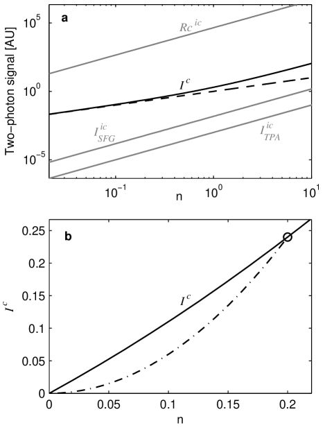
Figure 1: Power-dependence of the coherent and incoherent parts of two-photon interactions with down-converted light. (a) The relative magnitudes of the coherent signal $I^{c}$ (black line) vs. the incoherent signals for TPA, SFG and coincidence events ($I^{ic}_{\textsc{tpa}}$, $I^{ic}_{\textsc{sfg}}$ and $Rc^{ic}$, respectively, gray lines), assuming typical physical parameters described in the text, represented on a log-log scale. The graph shows the $n^{2}+n$ dependence of $I^{c}$, with $n$ being the average spectral photon density, i.e. the total photon flux in each of the signal and idler modes, divided by their bandwidth $\Delta$. All the incoherent signals demonstrate a quadratic dependence on $n$. The dashed line represents a completely linear function, for comparison. (b) The dependence of $I^{c}$ on $n$ represented on a linear scale, demonstrating the nearly linear dependence at small values of $n$. The dash-dot line depicts the quadratic response of $I^{c}$ assuming that down-converted light with $n=0.2$ is being attenuated by linear losses.

The first unique feature is the coherent signal’s non-classical linear intensity dependence: $I^{c}\propto n^{2}+n$. This behavior manifests the fact that the signal and idler modes share a single wavefunction. Figure 1 depicts this behavior of the coherent signal, compared to the quadratic intensity dependence of the incoherent signal. The relative magnitudes of the incoherent signals for SFG, TPA and coincidence events are calculated using Eqs. (68), (87) and (96), respectively (derived in the following subsections).

Note that while the dependence of the coherent signal on the flux of the down-converted photons may be linear, the response of the two-photon signal (TPA, SFG or coincidences) to attenuation of the down-converted light by linear losses (namely absorption or scattering, for example by optical filters or beam splitters) is always quadratic, as is evident from the presence of the term $\big{|}f_{avg}\big{|}^{2}$ in the expressions for both the coherent and incoherent signals. This behavior is depicted by the dash-dot line in Fig. 1, which assumes that down-converted light with average spectral photon density of $n=0.2$ is being attenuated by optical filters. These results are in excellent agreement with the experimental results of SFG with entangled photons presented in Dayan et al. (2005).

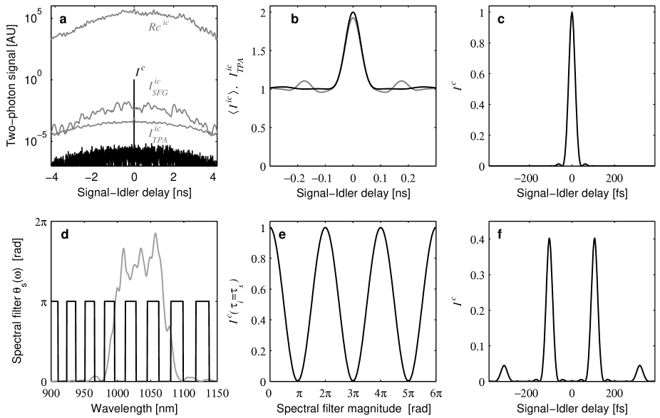
Figure 2: The temporal behavior of the coherent and incoherent parts of two-photon interactions with down-converted light, as a function of a relative delay between the signal and the idler fields. (a) The relative magnitudes of the coherent signal $I^{c}$ (black line) vs. the incoherent signals for TPA, SFG and coincidence events ($I^{ic}_{\textsc{tpa}}$, $I^{ic}_{\textsc{sfg}}$ and $Rc^{ic}$, respectively, gray lines), assuming typical physical parameters (described in the text), represented on a logarithmic scale. This graph depicts the instantaneous peak of the signals at $t=\tau_{i}$ for one typical down-converted pulse, and shows the contrast between the sharp temporal behavior of $I^{c}$, and the behavior of the incoherent signals, which is on the same ns-timescale as the pump pulse. Note that $I^{ic}_{\textsc{tpa}}$ presents a smooth and symmetric graph, reflecting fact that the long-lived ($\sim 30\>$ns) final atomic state integrates over the intensity variations of the pump pulse. Similarly, $Rc^{c}$, which takes into account integration over the gating time $Tg\sim 1\>$ns is more smooth than $I^{c}_{\textsc{sfg}}$, which represents an instantaneous parametric process. For the case assumed here of a non transform-limited $3\>$ns pump pulse, the ensemble average of all the incoherent signals becomes proportional to the normalized intensity-correlation function of the pump $\texttt{g}^{(2)}_{p}(\tau_{i}-\tau_{s})$, which exhibits a $\sim\times 2$ ’bunching peak’ at delays which are shorter than the pump’s coherence time $2\pi/\delta_{p}$. This is shown in (b) in black, together with the instantaneous incoherent TPA signal $I^{ic}_{\textsc{tpa}}$ (gray), which can be approximated to be proportional to $\texttt{g}^{(2)}_{p}$ even without averaging. (c) A zoomed-in presentation of the ultrashort-pulse like behavior of the coherent signal: $I^{c}(\tau_{i}-\tau_{s})\propto P_{e}(\tau_{i}-\tau_{s})$, assuming dispersion is compensated and no additional spectral filtering, resulting in a behavior that is identical to that of mixing two $35\>$fs transform-limited pulses. (e) $I^{c}$ at zero signal-idler delay as a function of the magnitude of a spectral phase filter $\theta_{s}(\omega)$ that is applied to the signal, for example by a pulse-shaper. $\theta_{s}(\omega)$ is drawn in (d) (black line) at a magnitude of $\pi$, together with the down-converted power spectrum (gray line). (f) The shaped temporal behavior of the coherent signal with $\theta_{s}(\omega)$ as depicted in (d) applied to the signal field.

The second unique feature that appears in Eq. (IV) is the pulse-like response of the coherent interaction to a relative delay between the signal and the idler, as represented by the term $P_{e}(\tau_{i}-\tau_{s})$, which is the (normalized) response of mixing two ultrashort pulses with practically the same spectra as the signal and idler. As such, $P_{e}(\tau_{i}-\tau_{s})$) is sensitive to dispersion, including the dispersion that was accumulated in the down-conversion process itself, denoted by the term $e^{-i\Delta k(\omega)L}$ in the definition of $P_{e}(\tau_{i}-\tau_{s})$ (Eq. (52)). Figure 2(c) shows a zoomed-in picture of this sharp temporal dependence of the coherent signal on relative delay between the signal and the idler beams, assuming that dispersion is either negligent or is compensated by spectral phase filters, leading to a sharp response which is exactly as if the interaction was induced by a pair of $35fs$ (transform-limited) pulses.

The coherent summation over the spectrum which leads to this pulse-like behavior also implies that the coherent signal can be shaped by spectral-phase manipulations, exactly like with coherent ultrashort pulses. Note that the shape of $P_{e}(\tau_{i}-\tau_{s})$ is determined by the sum of the phases applied to antisymmetric spectral components of the signal and the idler: $\theta_{s}(\omega)+\theta_{i}(\Omega_{0}-\omega)$. This implies that if the same phase filter is applied to both the signal and the idler beams (or the same dispersive medium), only spectral phase functions that are symmetric about $\Omega_{0}/2\approx\big{\langle}\omega_{p}\big{\rangle}/2$ would affect $P_{e}(\tau_{i}-\tau_{s})$. Figures 2(c)-(e) demonstrate how applying a spectral phase filter to the signal (or idler) spectrum leads to the same result as with coherent ultrashort pulses. This ultrashort-pulse-like behavior (including the ability to tailor it by a pulse-shaper) was demonstrated experimentally with high-power SFG in Dayan et al. (2003), high power TPA in Dayan et al. (2004), and with broadband entangled photons in Pe’er et al. (2005), with excellent agreement with our calculations.

Interestingly, $P_{e}(\tau_{i}-\tau_{s})$, does not depend on the specific type of the two-photon interaction, i.e. the coherent signal of TPA, SFG or coincidence events will always exhibit this ultrashort-pulse like behavior. The contrast between the temporal behavior of the coherent signal and that of the incoherent ones is shown in Fig. 2(a). Note that Fig. 2(a) presents the instantaneous peaks of the coherent and incoherent signals at $t=\tau_{i}$ for one, single-shot arbitrary example. As is evident, the incoherent signals (calculated for TPA, SFG and coincidence events by Eqs. (61), (79) and (95), respectively, assuming $n\gg 1$) always demonstrate a temporal dependence on $\tau_{s}-\tau_{i}$ that is on the same $ns$-timescale as the pump pulse.

It is important to note that the duration of such Q-switched pulses is much longer than their coherence time (which in this case is $2\pi/\delta_{p}\approx 89\>$ps), which was their duration if they were transform-limited. Such pump pulses, for which:

$$\tau_{p}\gg 2\pi/\delta_{p}\ ,$$ (56)

can be considered a ’quasi-continuous’ light, since they can be viewed as short bursts of continuous light, especially when time-scales that are shorter than $\tau_{p}$ are considered, during which the average intensity stays roughly constant. Thus, such quasi-continuous pump pulses yield approximately the same results for $I^{c}$, $I^{ic}$ as a continuous pump, especially when the ensemble average of many such pulses is considered. In particular, as will be shown in the next subsections, once averaged the incoherent signals all becomes proportional to the normalized second-order correlation function of the pump $\texttt{g}^{(2)}_{p}(\tau_{i}-\tau_{s})$. This behavior is depicted in Fig. 2(b), which depicts the calculated $\texttt{g}^{(2)}_{p}(\tau_{i}-\tau_{s})$ together with a zoomed-in presentation of the instantaneous incoherent TPA signal $I^{ic}_{\textsc{tpa}}$. As is evident, even without averaging $I^{ic}_{\textsc{tpa}}$ follows very closely $\texttt{g}^{(2)}_{p}(\tau_{i}-\tau_{s})$. This is explained by the fact that the incoherent excitation of the long-lived ($\sim 30\>$ns) final atomic state actually averages the intensity fluctuations of the pump (see Eq. (79)). When the ensemble average of many such quasi-continuous pulses is taken, the incoherent TPA signal, as well as $I^{ic}_{\textsc{sfg}}$ and $Rc^{ic}$ become practically identical to $\texttt{g}^{(2)}_{p}(\tau_{i}-\tau_{s})$, demonstrating the expected $\times 2$ ’bunching-peak’ at delays which are shorter than the coherence length of the pump $(\tau_{s}-\tau_{i}<1/\delta_{p})$ Mandel and Wolf (1995).

Another result of the temporal integration which is performed by the incoherent TPA process, is the fact that the behavior of $I^{ic}_{\textsc{tpa}}(\tau_{i}-\tau_{s})$ is more smooth and symmetric than that of $I^{ic}_{\textsc{sfg}}(\tau_{i}-\tau_{s})$, which represents an instantaneous process. Since coincidence measurement also includes a temporal integration over the $\sim 1\>$ns gating-time of the detectors, $Rc^{ic}$ presents a behavior which is more smooth and symmetric than $I^{ic}_{\textsc{sfg}}$, but not as much as $I^{ic}_{\textsc{tpa}}$.

Unlike the incoherent signals, the coherent signal’s sharp behavior $P_{e}(\tau_{i}-\tau_{s})$ depends on the large-scale properties of the down-converted spectrum, and therefore its shape is not affected by shot-to-shot noise, only its relative height. Thus, we see that there are three timescales in our system. One is the duration of the pump pulse (which can be infinity for a continuous pump), the other is the coherence time of the pump which is $\sim 1/\delta_{p}$ (and is equal to the duration of the pump pulse, in case it is a transform-limited one), and the shortest time scale is the behavior of the coherent signal, which is on the same timescale as the coherence time of the down-converted light: $1/\Delta$. In the case considered in Fig. 2, the $35fs$ pulse-like behavior of the coherent signal stands in contrast with the temporal behavior of the down-converted light itself, which is a $3ns$ pulse in this case, i.e. 85,000 times longer. The effect is of course even more intriguing when continuously-pumped down-conversion is considered.

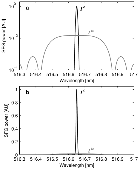
Figure 3: The spectrum of the coherent and incoherent parts of SFG light induced by high-power ($n\gg 1$) broadband down-converted light, with physical parameters as described in the text. The graphs are shown on a logarithmic scale in (a) and a linear scale in (b), and demonstrate how the coherent signal (black) replicates the narrow spectrum of the pump ($\delta_{p}=0.01nm$). In contrast, the spectrum of the incoherent signal (gray) is as wide as the phase-matching conditions at the crystal allow it to be ($\gamma_{\textsc{uc}}=0.3nm$).

The temporally-sharp behavior of the coherent signal also stands in contrast with its equally sharp spectral behavior. More specifically, we need to distinguish between two spectral behaviors. One is the excitation-spectrum, i.e. the frequencies which are excited by the two-photon interaction. The other is the dependence of the interaction on the pump wavelength. In the case of SFG, the excitation spectrum corresponds to the spectrum of the up-converted light. In the case of TPA this spectrum corresponds to which atomic levels will be excited. By Fourier-transforming the amplitude of the coherent signal in Eq. (IV) back to the frequency domain $\Omega$ of the generated signal, we see immediately that the excitation power-spectrum of the coherent signal is simply the spectral overlap between the narrowband pump and the final state, and does not reflect the broad spectra of the signal and the idler fields which induce the interaction:

$$I^{c}(\Omega,\tau_{s},\tau_{i}) \approx \big{|}f_{avg}\big{|}^{2}\>\frac{\Delta^{2}\>(n^{2}+n)}{I_{p}}\>P_{e}(\tau_{i}-\tau_{s})\>\bigg{|}g(\Omega-\Omega_{0})\>\textsf{A}_{p}(\Omega)\>e^{i\xi\tau_{i}}\bigg{|}^{2}\>.$$ (57)

This implies that if the pump bandwidth is narrower than the final state bandwidth, the excitation spectrum $I^{c}(\Omega)$ would follow that of the narrowband pump, as is shown for SFG in Fig. 3. In other words, the coherent signal behaves as if the pump itself was inducing the interaction. While the spectral behavior of the incoherent signal is harder to deduce out of Eq. (IV), in the following we show that it is approximately that of the final state; this is shown more easily if we assume the final state is significantly broader than the pump (Eq. (61)), or the other way around (Eq. (74)). This spectral behavior of the coherent and incoherent was demonstrated experimentally in Abram et al. (1986); Dayan et al. (2003).

For the case of TPA, even if the pump is narrower than the final atomic state, this is not reflected in the spectrum of the fluorescence from that level, because the temporally random, incoherent emission process of the emission erases the information on the exact frequency that drove the transition (especially in this limit of weak, non-stimulated interaction). However, while the excitation spectrum may not be directly accessible, the other kind of spectral behavior, i.e. the dependence of TPA on the pump wavelength, can be explored experimentally. As already evident from Eq. (IV), the magnitude of the coherent signal depends on the total spectral overlap between the pump spectrum and the final state spectrum. This is shown in Fig. 4, which considers TPA in atomic Rubidium (Rb) at the $5S_{1/2}-4D_{3/2,5/2}$ transition. The coherent TPA rate indeed behaves as if the pump laser itself was inducing the transition (which is of course a forbidden transition for a one-photon process), demonstrating a spectral resolution of 0.01nm, almost resolving the $13.4GHz$ hyperfine splitting between the $4D_{3/2}$ and the $4D_{5/2}$ levels, even though the interaction is induced by a light with a total bandwidth that is $\sim 2000$ times wider. For the sake of simplicity we ignored in Fig. 4 the hyperfine splitting of the $5S_{1/2}$ ground-level in Rb ($3GHz$ for Rb87, $6.8GHz$ for Rb85). This calculation should be compared with the experimental results of Dayan et al. (2004) (in which a wider pump bandwidth of $0.04nm$ and power-broadening prevented resolving the hyper-fine splitting, nonetheless demonstrating a spectral resolution that was $\sim 2000$ times narrower than the down-converted bandwidth). In contrast, the incoherent signal (for SFG, TPA and of course coincidence events) is practically independent of the wavelength of the pump (see Eq. (61) for SFG and Eq. (74) for TPA). The incoherent signal responds only to the change in the down-converted power spectrum that results from the change of the pump wavelength, and so it exhibits only the very wide spectral response that is expected in an interaction that is induced by mixing of two $80nm$ wide incoherent beams. This can be viewed as resulting from the fact that the incoherent interaction has no knowledge of what was the wavelength of the pump that generated the down converted light, since that ”information” lies only in the correlations between the spectral phases of the down-converted modes - phases that play no role in the generation of the incoherent signal.

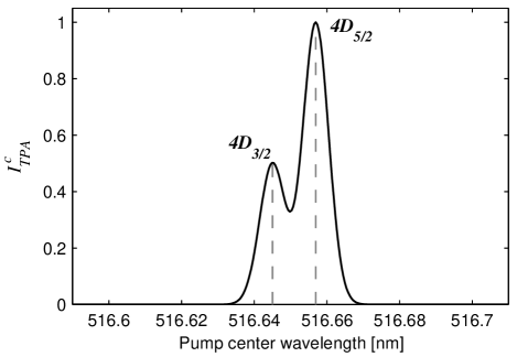
Figure 4: The dependence of the coherent part of TPA ($I^{c}_{\textsc{tpa}}$, black) induced by down-converted light, as a function of the center frequency of the pump. The graph shows how $I^{c}_{\textsc{tpa}}$ behaves as if the $0.01nm$-wide pump itself is inducing the transition ($5S_{1/2}$ $\rightarrow$ $4D_{3/2}$,$4D_{5/2}$ in atomic Rb, with the transition wavelengths drawn in gray). The incoherent part of the TPA is practically insensitive to the pump wavelength, and since for practical power levels ($n>1$) it is smaller than the coherent part by roughly $\delta_{p}/\Delta\approx 1/2000$ (with $\delta_{p}$, $\Delta$ being the bandwidths of the pump and the down-converted light, respectively), it is too small to appear in this graph.

In the following subsections we present more specific analytic expressions for the temporal behavior of the coherent and incoherent signals, performing approximations that fit various two-photon interactions. First we consider the case where the spectral width of the final state exceeds that of the pump, as is typically the case with SFG and is always the case with coincidence detection. Then we consider the case where the spectral width of the final state is smaller than that of the pump, as can occur with TPA. For more accurate results, and for experimental schemes that do not comply completely with the assumptions and approximations that follow, Eqs. (IV) or (IV) should be used.

V.2 Pump bandwidth smaller than the final-state bandwidth (example: SFG)

So far we have assumed that the down-converted bandwidth is significantly larger than the pump bandwidth and the final-state bandwidth (Eq. (48)). In the following derivation we consider the case where the pump bandwidth is also significantly narrower than the final-state bandwidth:

$$\Delta\gg\gamma\gg\delta_{p}\ .$$ (58)

This condition allows us to simplify the expressions for both the coherent and the incoherent signals from Eq. (IV) by using the following approximation:

$$\int_{\gamma}d\xi\>g(\xi)\>\textsf{A}_{p}(\bar{\omega}+\xi)\>e^{-i\xi(t-\tau_{i})} \approx \sqrt{2\pi}\>g(\langle\omega_{p}\rangle-\bar{\omega})\>A_{p}(t-\tau_{i})\>e^{i\bar{\omega}(t-\tau_{i})}\ ,$$ (59)

where $A_{p}(t)=\emph{F}^{-1}\big{\{}\textsf{A}_{p}(\omega)\big{\}}$ is the temporal amplitude of the pump, leading quite immediately to:

$$I^{c}(t-\tau_{i},\tau_{i}-\tau_{s}) \approx \big{|}g(\langle\omega_{p}\rangle-\Omega_{0})\big{|}^{2}\>\big{|}f_{avg}\big{|}^{2}\>\frac{\texttt{I}_{p}(t-\tau_{i})}{I_{p}}\>\Delta^{2}\>(n^{2}+n)\>P_{e}(\tau_{i}-\tau_{s})\ .$$ (60)

$$I^{ic}(t-\tau_{i},\tau_{i}-\tau_{s}) \approx \ \int_{\gamma}d\xi^{\prime}\big{|}g(\xi^{\prime})\big{|}^{2}\>\ \big{|}f_{avg}\big{|}^{2}\>\frac{\texttt{I}_{p}(t-\tau_{i})\texttt{I}_{p}(t-\tau_{s})}{I_{p}^{2}}\>\Delta\>n^{2}\ ,$$ (61)

with $\texttt{I}_{p}(t)=|A_{p}(t)|^{2}$. To represent more accurately typical experimental conditions, we can take the ensemble average of the signals (i.e. averaging over many pulses in the case of a pulsed pump, or over time in the case of a continuous pump). In particular, if we consider a continuous pump or a quasi-continuous pump (i.e. the center part of a non-transform-limited pump pulse for which $\tau_{p}\gg 2\pi/\delta_{p}$), we can approximate for $t-\tau_{s},t-\tau_{i}\ll\tau_{p}$:

$$\big{\langle}\texttt{I}_{p}(t-\tau_{i})\big{\rangle}\approx\big{\langle}\texttt{I}_{p}(t-\tau_{i})\big{\rangle}\approx\big{\langle}\texttt{I}_{p}(0)\big{\rangle}\approx I_{p}\ .$$ (62)

This allows us to further simplify the expressions for the coherent and incoherent signals by using:

$$\frac{\big{\langle}\texttt{I}_{p}(t-\tau_{i})\big{\rangle}}{I_{p}} \approx 1\ ,$$ (63)

$$\frac{\big{\langle}\texttt{I}_{p}(t-\tau_{i})\texttt{I}_{p}(t-\tau_{s})\big{\rangle}}{I_{p}^{2}} \approx \frac{\big{\langle}\texttt{I}_{p}(t-\tau_{i})\texttt{I}_{p}(t-\tau_{s})\big{\rangle}}{\big{\langle}\texttt{I}_{p}(t-\tau_{i})\big{\rangle}\big{\langle}\texttt{I}_{p}(t-\tau_{s})\big{\rangle}}=\texttt{g}^{2}_{p}(\tau_{i}-\tau_{s})\ ,$$ (64)

where $\texttt{g}^{2}_{p}(\tau_{i}-\tau_{s})$ is the normalized second-order correlation function of the pump field. Note that the pump field was taken as a classical amplitude throughout this paper, hence $\texttt{g}^{2}_{p}$ represents in our derivation only classical intensity correlations. This leads to:

$$\big{\langle}I^{c}(t-\tau_{i},\tau_{i}-\tau_{s})\big{\rangle} \approx \big{|}g(\langle\omega_{p}\rangle-\Omega_{0})\big{|}^{2}\>\big{|}f_{avg}\big{|}^{2}\>\Delta^{2}\>(n^{2}+n)\>P_{e}(\tau_{i}-\tau_{s})\ .$$ (65)

$$\big{\langle}I^{ic}(t-\tau_{i},\tau_{i}-\tau_{s})\big{\rangle} \approx \ \int_{\gamma}d\xi^{\prime}\big{|}g(\xi^{\prime})\big{|}^{2}\>\ \big{|}f_{avg}\big{|}^{2}\>\texttt{g}^{2}_{p}(\tau_{i}-\tau_{s})\>\Delta\>n^{2}\ .$$ (66)

As is reflected in the term $\int_{\gamma}d\xi^{\prime}\big{|}g(\xi^{\prime})\big{|}^{2}$ in Eqs. (61), (66), the power of the incoherent signal is indeed the incoherent summation of all its spectral components, and its spectrum follows that of the final state. This behavior is depicted in Fig. 3 for SFG, in which case we may write:

$$\big{|}f_{avg}\big{|}^{2}\ \big{|}g(\Omega-\Omega_{0})\big{|}^{2}=L^{2}\>\textrm{sinc}^{2}\big{[}\Delta k(\langle\omega\rangle,\Omega)L/2\big{]}\>\beta^{2}(\langle\omega\rangle,\Omega)\ .$$ (67)

With the exception of very long crystals (i.e. more than $\sim 1$ cm in the case of type-I up conversion, or more than a few mm in the case of type-II up conversion), the up-converted bandwidth $\gamma_{\textsc{uc}}$ is typically at least of the order of $0.01\>$THz, and could even reach tens of THz for very short crystals. This bandwidth is orders of magnitude larger than the typical bandwidth of continuous lasers, and even larger than the bandwidth of Q-switched, $ns$-pulsed lasers. Thus, the condition of Eq. (58) is typically satisfied for SFG, unless ultrashort pulses (hundreds of $fs$ or less) are used.

Equations 61,66 displays both the spectral and the temporal behaviors of the incoherent signal more clearly than Eq. (IV) did. As is evident, the incoherent signal is practically insensitive to the pump wavelength, and its response to a relative delay between the signal and the idler is very slow, since it depends on the temporal behavior of the pump, which is either continuous or a very long pulse, compared to the ultrashort-pulse-like behavior of the coherent signal; as demonstrated by the term $\texttt{I}_{p}(t-\tau_{i})\texttt{I}_{p}(t-\tau_{s})$, the incoherent signal depends only on the temporal overlap between the intensities of the signal and the idler (which follow the intensity of the pump). This behavior is depicted in Fig. 2(a)-(c). In particular, Fig. 2(b) shows the ’bunching’ peak which is exhibited by the incoherent signal for a quasi-continuous pump at delays which are shorter than the pump’s coherence length.

Since the observed signal is always the sum of the coherent and incoherent contributions, it interesting to compare the magnitude of the coherent signal to that of the incoherent one. The average ratio between the coherent signal and the incoherent one is therefore:

$$\frac{\big{\langle}I^{c}(t-\tau_{i},\tau_{i}-\tau_{s})\big{\rangle}}{\big{\langle}I^{ic}(t-\tau_{i},\tau_{i}-\tau_{s})\big{\rangle}} \approx \frac{\big{\langle}\texttt{I}_{p}(t-\tau_{i})\big{\rangle}\>I_{p}}{\big{\langle}\texttt{I}_{p}(t-\tau_{i})\texttt{I}_{p}(t-\tau_{s})\big{\rangle}}\frac{\Delta}{\gamma}\>\frac{(n^{2}+n)}{n^{2}}\>P_{e}(\tau_{i}-\tau_{s})\ ,$$ (68)

which for a continuous or quasi-continuous pump becomes:

$$\frac{\big{\langle}I^{c}(t-\tau_{i},\tau_{i}-\tau_{s})\big{\rangle}}{\big{\langle}I^{ic}(t-\tau_{i},\tau_{i}-\tau_{s})\big{\rangle}} \approx \frac{\Delta}{\gamma\>\texttt{g}^{2}_{p}(\tau_{i}-\tau_{s})}\>\frac{(n^{2}+n)}{n^{2}}\>P_{e}(\tau_{i}-\tau_{s})\ .$$ (69)

In the absence of spectral phase filters, and assuming that dispersion is corrected, we can assign $P_{e}(0)=1$. Thus, taking into account that typically $1\leq\texttt{g}^{2}_{p}(\tau_{i}-\tau_{s})\leq 2$, the expected ratio between the coherent and incoherent signals approaches $\Delta/\gamma$ for high powers ($n>1$), and even more for low powers where $n+n^{2}\gg n^{2}$. Thus, under the conditions of broadband down conversion and a narrowband final state assumed throughout our derivation, the coherent signal dominates over the incoherent signals (see the relative magnitude of $I^{ic}_{\textsc{sfg}}$ in Figs. 1-3).

V.3 Pump bandwidth larger than the final-state bandwidth (example: TPA)

For the following derivation we assume that the final-state bandwidth $\gamma$ is significantly narrower than the pump bandwidth, as may often be the case with TPA:

$$\Delta\gg\delta_{p}\gg\gamma\ .$$ (70)

Assuming this, we can simplify the expressions from Eq. (IV) by assuming that the spectral amplitude of the pump remains constant within spectral slices which are narrower than $\gamma$ :

$$\textsf{A}_{p}(\bar{\omega}+\xi) \approx \textsf{A}_{p}(\bar{\omega})\ .$$ (71)

Additionally, in order to evaluate the incoherent TPA signal we use Parseval’s theorem to obtain the following relation:

$$\int^{\infty}_{0}d\upsilon\>\bigg{|}\int_{0}^{\infty}d\omega_{p}\>\textsf{A}_{p}(\omega_{p})\>\textsf{A}_{p}(\upsilon-\omega_{p})e^{i\omega_{p}\tau}\bigg{|}^{2} = 2\pi\int_{-\infty}^{\infty}\texttt{I}_{p}(t^{\prime}+\tau)\texttt{I}_{p}(t^{\prime})\>dt^{\prime}\ ,$$ (72)

leading to:

$$I^{c}(t-\tau_{i},\tau_{i}-\tau_{s}) \approx \big{|}f_{avg}\big{|}^{2}\>\big{|}\textsf{A}_{p}(\Omega_{0})\big{|}^{2}\>\frac{\Delta^{2}\>(n^{2}+n)}{2\pi I_{p}}\>\bigg{|}\int_{\gamma}d\xi\>g(\xi)\>e^{-i\xi(t-\tau_{i})}\>\bigg{|}^{2}\>P_{e}(\tau_{i}-\tau_{s})$$ (73)

$$I^{ic}(t-\tau_{i},\tau_{i}-\tau_{s}) \approx \big{|}f_{avg}\big{|}^{2}\>\frac{\Delta\>n^{2}}{2\pi I_{p}^{2}}\ \int_{-\infty}^{\infty}\texttt{I}_{p}(t^{\prime}+\tau)\texttt{I}_{p}(t^{\prime})\>dt^{\prime}\>\ \bigg{|}\int_{\gamma}d\xi\ g(\xi)\>e^{-i\xi(t-\tau_{i})}\bigg{|}^{2}\ .$$ (74)

Equations 73-74 show that in this case the spectra of both the coherent and the incoherent signals are determined by the spectrum of the final state $g(\xi)$.

To clarify the temporal behavior of both signals, let us use

$$\int_{\gamma}d\xi\ g(\xi)\>e^{-i\xi(t-\tau_{i})}=G(t-\tau_{i})\ ,$$ (75)

with $G(t)=\emph{F}^{-1}\big{\{}g(\xi)\big{\}}$ being the slowly varying envelope of the temporal response of the final state. This leads to:

$$I^{c}(t-\tau_{i},\tau_{i}-\tau_{s}) \approx \big{|}f_{avg}\big{|}^{2}\>\big{|}\textsf{A}_{p}(\Omega_{0})\big{|}^{2}\>\frac{\Delta^{2}\>(n^{2}+n)}{I_{p}}\>\big{|}G(t-\tau_{i})\big{|}^{2}\>P_{e}(\tau_{i}-\tau_{s})$$ (76)

$$I^{ic}(t-\tau_{i},\tau_{i}-\tau_{s}) \approx \big{|}f_{avg}\big{|}^{2}\>\frac{\Delta\>n^{2}}{I_{p}^{2}}\ \int_{-\infty}^{\infty}\texttt{I}_{p}(t^{\prime}+\tau)\texttt{I}_{p}(t^{\prime})\>dt^{\prime}\>\ \big{|}G(t-\tau_{i})\big{|}^{2}\ .$$ (77)

Considering TPA as a probable example for the case where the final state is considerably narrower than the pump, we can substitute $g(\xi)=\frac{1}{\xi+i\gamma}$. Using $\emph{F}^{-1}\big{\{}g(\xi)\big{\}}=\textsc{u}(t-\tau_{i})\>e^{-\gamma_{h}(t-\tau_{i})}$ (where $\textsc{u}(t)$ is a step-function), we obtain for TPA:

$$I^{c}(t-\tau_{i},\tau_{i}-\tau_{s}) = \kappa_{\textsc{tpa}}\>\frac{\big{|}\textsf{A}_{p}(\Omega_{0})\big{|}^{2}}{I_{p}}\>\textsc{u}(t-\tau_{i})\>e^{-2\gamma_{f}(t-\tau_{i})}\>\Delta^{2}\>(n^{2}+n)\>P_{e}(\tau_{i}-\tau_{s})$$ (78)

$$I^{ic}(t-\tau_{i},\tau_{i}-\tau_{s}) = \kappa_{\textsc{tpa}}\>\frac{\int_{-\infty}^{\infty}\texttt{I}_{p}(t^{\prime}+\tau_{s}-\tau_{i})\texttt{I}_{p}(t^{\prime})\>dt^{\prime}}{I_{p}^{2}}\>\textsc{u}(t-\tau_{i})\>e^{-2\gamma_{f}(t-\tau_{i})}\>\Delta\>n^{2}\ ,$$ (79)

with

$$\kappa_{\textsc{tpa}}=\frac{1}{32\pi^{3}}\bigg{[}\frac{\sum_{n}\mu_{fn}\mu_{ng}}{c\varepsilon S\hbar}\bigg{]}^{2}\frac{\langle\omega\rangle(\omega_{fg}-\langle\omega\rangle)}{(\omega_{ng}-\langle\omega\rangle)^{2}}\ .$$ (80)

In order to have a better estimation of the magnitude of the coherent TPA signal as compared to the incoherent one, let us try to estimate the average magnitude of $\big{|}\textsf{A}_{p}(\Omega_{0})\big{|}^{2}$, assuming of course that $\Omega_{0}$ is within the pump spectrum (i.e. $|\Omega_{0}-\langle\omega_{p}\rangle|<\delta_{p}/2$). For a pulsed pump, we can use Parseval’s theorem again to relate between the average spectral power of the pump $\big{\langle}|\texttt{A}_{p}|^{2}\big{\rangle}$ to the average temporal power $I_{p}$:

$$\delta_{p}\>\langle\big{|}\textsf{A}_{p}\big{|}^{2}\rangle = \tau_{p}\>I_{p}\ .$$ (81)

However, to get a similar relation for a continuous pump we need to identify the longest timescale in our system, which defines the smallest frequency increment, i.e. the quantization unit of our frequency domain. In the case considered in this subsection, the smallest frequency scale is that of the final state, $\gamma_{f}$ (Eq. (70)), hence the longest relevant timescale is the final state lifetime $\tau_{f}$. Accordingly we can approximate for a continuous pump:

$$\delta_{p}\>\langle\big{|}\textsf{A}_{p}\big{|}^{2}\rangle \approx \tau_{f}\>I_{p}\ ,$$ (82)

which is identical to Eq. (81), only with $\tau_{f}$ replacing $\tau_{p}$. In other words, although the pump is continuous, we can treat it as if it was composed of serious of pulses, each of them $\tau_{f}$ long. Since the atomic state, which is the slowest component in our system, has a ”memory” only $\tau_{f}$ long, its response is not affected by interactions that occurred more than $\tau_{f}$ seconds ago. All the other components of our system have shorter coherence time; for example, since the pulse bandwidth is significantly wider than $\gamma_{f}=2\pi/\tau_{f}$, it is not affected by such ’chopping’ of continuous light to pulses $\tau_{f}$ long. Using Eq. (82), and assuming the final state is included within the pump spectrum, we get:

$$I^{c}(t-\tau_{i},\tau_{i}-\tau_{s}) \approx \kappa_{\textsc{tpa}}\>\frac{\tau_{f}}{\delta_{p}}\>\textsc{u}(t-\tau_{i})\>e^{-2\gamma_{f}(t-\tau_{i})}\>\Delta^{2}\>(n^{2}+n)\>P_{e}(\tau_{i}-\tau_{s})\ ,$$ (83)

and the ratio between the coherent and the incoherent signals is therefore:

$$\frac{I^{c}(t-\tau_{i},\tau_{i}-\tau_{s})}{I^{ic}(t-\tau_{i},\tau_{i}-\tau_{s})} \approx \frac{I_{p}^{2}}{\int_{-\infty}^{\infty}\texttt{I}_{p}(t^{\prime}+\tau_{s}-\tau_{i})\texttt{I}_{p}(t^{\prime})\>dt^{\prime}}\>\frac{\Delta}{\delta_{p}}\ \frac{n^{2}+n}{n^{2}}\>P_{e}(\tau_{i}-\tau_{s})\ .$$ (84)

Similarly to the case with SFG, we see that the coherent signal is stronger than the incoherent one (in the absence of dispersion or delay between the signal and idler), this time roughly by the ratio between the down-converted bandwidth and the pump bandwidth $\Delta/\delta_{p}$.

To clarify the dependence of the incoherent signal on a relative delay between the signal and the idler, let us consider the case of a continuous, stationary pump, for which $\big{\langle}\texttt{I}_{p}(t+\tau)\big{\rangle}=\big{\langle}\texttt{I}_{p}(t)\big{\rangle}=I_{p}$, and so the intensity correlations can be represented by the normalized second-order correlation function of the pump:

$$\frac{\int_{\tau_{f}}\texttt{I}_{p}(t^{\prime}+\tau_{s}-\tau_{i})\texttt{I}_{p}(t^{\prime})\>dt^{\prime}}{I_{p}^{2}}\approx\tau_{f}\>\frac{\big{\langle}\texttt{I}_{p}(t+\tau_{s}-\tau_{i})\texttt{I}_{p}(t)\big{\rangle}}{\big{\langle}\texttt{I}_{p}(t+\tau_{s}-\tau_{i})\big{\rangle}\big{\langle}\texttt{I}_{p}(t)\big{\rangle}}=\tau_{f}\>\texttt{g}^{(2)}_{p}(\tau_{i}-\tau_{s})\ ,$$ (85)

where $\tau_{f}$ is the lifetime of the atomic $|f\rangle$ state, which is the physical time interval over which the intensity correlations are actually integrated. Equation 85 is valid as long as the lifetime of the final state is much longer than the coherence time of the pump, which is indeed the case considered here since we assumed $\delta_{p}\gg\gamma$. Therefore we may write:

$$I^{ic}(t-\tau_{i},\tau_{i}-\tau_{s}) \approx \kappa_{\textsc{tpa}}\>\tau_{f}\ \texttt{g}^{(2)}_{p}(\tau_{i}-\tau_{s})\>\textsc{u}(t-\tau_{i})\>e^{-2\gamma_{f}(t-\tau_{i})}\>\Delta\>n^{2}\ ,$$ (86)

and the ratio between the coherent and incoherent signals then becomes:

$$\frac{I^{c}(t-\tau_{i},\tau_{i}-\tau_{s})}{I^{ic}(t-\tau_{i},\tau_{i}-\tau_{s})} \approx \frac{1}{\texttt{g}^{(2)}_{p}(\tau_{i}-\tau_{s})}\>\frac{\Delta}{\delta_{p}}\ \frac{n^{2}+n}{n^{2}}\>P_{e}(\tau_{i}-\tau_{s})\ .$$ (87)

If the final state is inhomogeneously broadened with an inhomogeneous bandwidth $\gamma_{\textsc{ih}}$, we may use Eq. (39) to obtain (assuming this time that $\gamma_{\textsc{ih}}>\delta_{p}$):

$$I_{\textsc{ih}}^{c}(t-\tau_{i},\tau_{i}-\tau_{s}) \approx \kappa_{\textsc{tpa}}\>\tau_{f}\>\textsc{u}(t-\tau_{i})\>e^{-2\gamma_{f}(t-\tau_{i})}\>\Delta^{2}\>(n^{2}+n)\>P_{e}(\tau_{i}-\tau_{s})$$

$$I_{\textsc{ih}}^{ic}(t-\tau_{i},\tau_{i}-\tau_{s}) \approx \kappa_{\textsc{tpa}}\>\tau_{f}\>\texttt{g}^{(2)}_{p}(\tau_{i}-\tau_{s})\>\textsc{u}(t-\tau_{i})\>e^{-2\gamma_{f}(t-\tau_{i})}\>\gamma_{\textsc{ih}}\>\Delta\>n^{2}\ ,$$ (88)

and the ratio between the coherent and the incoherent signals is then the same as in Eq. (87), only with $\gamma_{\textsc{ih}}$ replacing $\delta_{p}$.

Similar results can be obtained for a quasi-continuous pump, i.e. if we consider the ensemble average of non transform-limited pulses, for which we may write (for small delays, $\tau_{i}-\tau_{s}\ll\tau_{p}$):

$$\bigg{\langle}\frac{\int_{\tau_{f}}\texttt{I}_{p}(t^{\prime}+\tau_{s}-\tau_{i})\texttt{I}_{p}(t^{\prime})\>dt^{\prime}}{I_{p}^{2}}\bigg{\rangle}\approx\tau_{p}\>\texttt{g}^{(2)}_{p}(\tau_{i}-\tau_{s})\ .$$ (89)

This leads to the same results as with a continuous pump, with the only difference being that $\tau_{p}$ is replacing $\tau_{f}$:

$$\big{\langle}I^{c}(t-\tau_{i},\tau_{i}-\tau_{s})\big{\rangle} \approx \kappa_{\textsc{tpa}}\>\frac{\tau_{p}}{\delta_{p}}\>\textsc{u}(t-\tau_{i})\>e^{-2\gamma_{f}(t-\tau_{i})}\>\Delta^{2}\>(n^{2}+n)\>P_{e}(\tau_{i}-\tau_{s})$$ (90)

$$\big{\langle}I^{ic}(t-\tau_{i},\tau_{i}-\tau_{s})\big{\rangle} \approx \kappa_{\textsc{tpa}}\>\tau_{p}\ \texttt{g}^{(2)}_{p}(\tau_{i}-\tau_{s})\>\textsc{u}(t-\tau_{i})\>e^{-2\gamma_{f}(t-\tau_{i})}\>\Delta\>n^{2}\ ,$$ (91)

and the ratio between the average coherent and the average incoherent signals therefore remains the same as in 87. Accordingly, in the case of inhomogeneous broadening the same results hold, with $\tau_{p}$ replacing $\tau_{f}$ there as well.

V.4 Coincidence events

It is quite intriguing to compare the results obtained for SFG and TPA with down-converted light to the expected rate $Rc$ of coincidence events, i.e. the simultaneous arrival of signal and idler photons. Typically, the coincidence rate is evaluated as proportional to the second-order correlation function $\texttt{g}^{(2)}(\tau)$. If the temporal response of the coincidence detectors (and the corresponding electronics) is slower than the coherence time of the photons ($\sim 1/\Delta$), as is typically the case, then it is taken into account by integrating over the gating time $Tg$ :

$$Rc\propto\int_{Tg}\texttt{g}^{(2)}(\tau)\>d\tau\ .$$ (92)

In order to obtain an approximated expression for the coincidence rate, we will use the spectral functions $g(\xi),f(\omega,\Omega_{0})$ defined in Eq. (III.3). Essentially, this means that we treat coincidence detection as if it was an SFG process with a very large up-converted bandwidth $\gamma_{\textsc{uc}}$:

$$\gamma_{\textsc{uc}}=2\>\Delta\ .$$ (93)

Intuitively speaking, such SFG process may be considered as equivalent to coincidence detection since any pair of photons that arrives at the crystal simultaneously (i.e. with a temporal separation that is smaller than their coherence time $\sim 1/\Delta$) has an equal probability to be up-converted, regardless of the frequency of the resulting up-converted photon. Although we have previously assumed that $\gamma_{\textsc{uc}}\ll\Delta$ (Eq. (48)), this assumption was made only to allow the neglect of the spectral variations of $n_{s,i}(\omega)$. Therefore, if we limit our discussion to down-converted spectrum that its average is approximately smooth, we may use the expressions obtained for SFG to describe $\texttt{g}^{(2)}(\tau_{s}-\tau_{i})$, simply by replacing $\gamma_{\textsc{uc}}$ by $2\Delta$:

$$\texttt{g}^{(2)}(\tau_{s}-\tau_{i}) \propto \frac{\texttt{I}_{p}(t-\tau_{i})}{I_{p}}\>\Delta^{2}\>(n^{2}+n)\>P_{e}(\tau_{i}-\tau_{s})$$ (94)

$$+ \frac{\texttt{I}_{p}(t-\tau_{i})\texttt{I}_{p}(t-\tau_{s})}{I_{p}^{2}}\>2\>\Delta^{2}\>n^{2}\ ,$$

where the first term represents the coherent contribution, and the second represents the incoherent one. However, $\texttt{g}^{(2)}(\tau_{s}-\tau_{i})$ represents the actual coincidence detection rate only for infinitely fast detectors; for broadband radiation the temporal resolution of the coincidence detectors is typically orders of magnitude longer than the coherence time of the photons. Therefore, applying Eq. (92) and taking $Tg\gg 1/\Delta,|\tau_{s}-\tau_{i}|$, we obtain:

$$Rc^{c} \propto \frac{\texttt{I}_{p}(t-\tau_{i})}{I_{p}}\>\Delta\>(n^{2}+n)\>P_{e}(\tau_{i}-\tau_{s})$$

$$Rc^{ic} \propto \frac{\texttt{I}_{p}(t-\tau_{i})\texttt{I}_{p}(t-\tau_{s})}{I_{p}^{2}}\>2\>Tg\>\Delta^{2}\>n^{2}\ .$$ (95)

As with TPA or SFG if a temporal averaging is performed for the case of a continuous pump, or an ensemble average is performed with quasi-continuous, long pump pulses, the ratio $\big{\langle}{\texttt{I}_{p}(t-\tau_{i})}/{I_{p}}\big{\rangle}$ in the coherent term approaches 1, and the ratio $\big{\langle}{\texttt{I}_{p}(t-\tau_{i})\texttt{I}_{p}(t-\tau_{s})}/{I_{p}^{2}}\big{\rangle}$ in the incoherent term approaches $\texttt{g}^{2}_{p}(\tau_{i}-\tau_{s})$ (for small delays). Thus the ratio between the average coherent and the incoherent contributions becomes:

$$\frac{Rc^{c}}{Rc^{ic}} \approx \frac{1}{\texttt{g}^{2}_{p}(\tau_{i}-\tau_{s})}\frac{1}{2Tg\>\Delta}\ \frac{(n^{2}+n)\>P_{e}(\tau_{i}-\tau_{s})}{n^{2}}\ .$$ (96)

Since at any power level down-converted light is essentially composed of simultaneously-created photon pairs, it is natural to assume that it will exhibit high degree of bunching, in the sense that there will always be a significantly higher rate of simultaneous arrivals of photons from the signal and the idler beams (at zero delay), as compared to Poissonian or even thermal distributions. However (and counter-intuitively), as is evident from Eqs. (V.4)-(96), since $Tg\gg 1/\Delta$, at high power levels ($n\geq 1$) the coincidence rate is dominated by the incoherent term, which exhibits similar bunching properties as those of the pump; thus, unlike the frequency-selective processes of SFG and TPA, the coherent contribution to the coincidence rate is dominant only at the very low power levels of $n\ll 1$, where down-converted light can be described as a stream of entangled photon pairs.

VI Summary and conclusions

In this paper we derived expressions for two-photon interactions induced by broadband down-converted light that was pumped by a narrowband laser. In section II we solved the equations of motion for the annihilation and creation operators of broadband down-converted light generated by an arbitrary narrowband pump. In section III we formulated operators that represent the photon flux or the probability amplitude of weak two-photon interactions (i.e. assuming low efficiency of the interaction, so that the inducing fields are not depleted) induced by arbitrary broadband light. In section IV we combined the results of the previous sections to obtain expressions for the intensities of two-photon interactions, namely SFG, TPA and coincidence events, induced by broadband down-converted light, and in section V we explored their temporal and spectral behaviors under various conditions.

Our calculations show that the intensity of two-photon interactions induced by broadband down-converted light can be represented as the sum of two terms, one ($I^{c}$) that exhibits a coherent behavior, and a second one ($I^{ic}$) that exhibits an incoherent behavior:

$$I^{total}=I^{c}+I^{ic}\ .$$ (97)

The two terms vary dramatically both in their spectral properties, as well as in their temporal properties. We considered the case where the signal and the idler may propagate freely along different optical paths from the down-converting crystal, accumulating independent temporal delays $\tau_{s}$, $\tau_{i}$ before inducing the two-photon interaction. The coherent signal then responds to a relative delay between the signal and the idler in an ultrashort-pulse like behavior:

$$I^{c}(t,\tau_{s},\tau_{i})\propto\texttt{I}_{p}(t-\tau_{i})\>P_{e}(\tau_{i}-\tau_{s})\ ,$$ (98)

where $\texttt{I}_{p}(t)$ is the power of the pump (in units of photon flux), and $P_{e}(\tau_{i}-\tau_{s})$ is the temporal response one would have got if the two-photon interaction was induced by mixing two ultrashort, transform-limited pulses with the same power spectra as the signal and the idler, although the signal and the idler are each incoherent and may even be continuous (see Fig. 2(c)). Accordingly, $P_{e}(\tau_{i}-\tau_{s})$ is sensitive to dispersion just as a coherent ultrashort pulse (including the dispersion of the down-conversion process itself), and can even be shaped by conventional pulse-shaping techniques (see Figs. 2(d)-(f)). Note that at low powers this corresponds to shaping of the second-order correlation function $\texttt{g}^{(2)}$ of the down-converted entangled photon pairs. It is also interesting to note that $P_{e}(\tau_{i}-\tau_{s})$ responds to the antisymmetric sum of the phases applied to the signal and the idler: $\theta_{s}(\omega)+\theta_{i}(\langle\omega_{p}\rangle-\omega)$, with $\langle\omega_{p}\rangle$ being the center frequency of the pump. Thus, if the same spectral filter is applied to both the signal and the idler beams, only phase functions that are symmetric about $\langle\omega_{p}\rangle/2$ affect $P_{e}$. Similarly, if the signal and the idler travel through the same medium, only odd orders of dispersion will have an effect on $P_{e}$.

In contrast, the incoherent signal depends only on the temporal overlap between the intensities of the down-converted signal and idler beams, and so reacts to a delay between the signal and the idler on the same time-scale as the long pulses or even continuous behavior of the pump:

$$I^{ic}(t,\tau_{s},\tau_{i})\propto\texttt{I}_{p}(t-\tau_{i})\texttt{I}_{p}(t-\tau_{s})$$ (99)

if the pump is narrower than the final state, or

$$I^{ic}(t,\tau_{s},\tau_{i})\propto\int_{-\infty}^{\infty}\texttt{I}_{p}(t^{\prime}+\tau_{s}-\tau_{i})\texttt{I}_{p}(t^{\prime})\>dt^{\prime}\ ,$$ (100)

if the final state is narrower than the pump. In both cases, if we consider the temporal average in the case of a continuous pump, or the ensemble average in the case of a quasi-continuous pump (i.e. non-transform limited pulses, for which $\tau_{p}\gg 2\pi/\delta_{p}$, with $\tau_{p}$ being the duration of the pulses, and $\delta_{p}$ their bandwidth), then the average incoherent signal is proportional to the normalized second-order correlation function of the pump (for $\tau_{i}-\tau_{s}\ll\tau_{p}$):

$$\big{\langle}I^{ic}(t,\tau_{s},\tau_{i})\big{\rangle}\propto\texttt{g}^{2}_{p}(\tau_{i}-\tau_{s})\ .$$ (101)

Thus, as depicted in Fig. 2, there are three temporal timescales in our system. The longest one is the duration of the pump pulse (which can be infinity for a continuous pump). This timescale dictates the temporal behavior of the incoherent signal as a function of the signal-idler delay. The next is the coherence time of the pump which is $\sim 1/\delta_{p}$ (and is equal to the duration of the pump pulse, in case it is a transform-limited one). For signal-idler delays which are shorter than this coherence time, the average of the incoherent signal is higher since the intensities of the signal and the idler become correlated, as they both reflect the intensity fluctuations of the pump. The shortest time scale is the behavior of the coherent signal, which is on the same timescale as the coherence time of the broadband down-converted light: $1/\Delta$.

As for the spectral behavior, the coherent signal behaves as though the interaction is actually being induced by the pump itself, and not by the down-converted light. Thus, the coherent signal is induced only if the pump spectrum overlaps with the final state:

$$I^{c}(\Omega_{0}+\xi)\propto\bigg{|}\int_{\gamma}d\xi\>g(\xi)\>\textsf{A}_{p}(\Omega_{0}+\xi)\>\bigg{|}^{2}\ ,$$ (102)

where $g(\xi)$ represents the the spectrum of the final atomic level in TPA, or the phase-matching function for up-conversion in the case of SFG, and with $\Omega_{0}$ being the center frequency of the final atomic level or of the phase-matched spectrum in case of SFG. The consequences of this spectral behavior is that by scanning the pump wavelength we can perform two-photon spectroscopy with the spectral resolution of the narrowband pump, even though the interaction is induced by light that is orders of magnitude wider than the pump, and not by the pump itself (see Fig. 4). In the case of SFG this means that light is being up converted only at those wavelengths:

$$I^{c}_{\textsc{sfg}}(\Omega_{0}+\xi)\propto\big{|}g(\xi)\>\textsf{A}_{p}(\Omega_{0}+\xi)\>\big{|}^{2}\ ,$$ (103)

so that even if the phase matching conditions allow broadband up-conversion, $I^{c}_{\textsc{sfg}}$ replicates the narrow spectrum of the pump (see Fig. 3).

The incoherent signal, on the other hand, is insensitive to the exact wavelength of the pump that generated the down-converted light. Since the information on the original wavelength of the pump is imprinted in the phase correlations between the down-converted modes, it affects only the coherent signal $I^{c}$. Accordingly, the incoherent signal is induced at all the possible frequency band of the final state of the interaction (see Fig. 3):

$$I^{ic}(\Omega_{0}+\xi)\propto\big{|}g(\xi)\big{|}^{2}\ .$$ (104)

The coherent and incoherent signals also exhibit different dependencies on $n$, the average photon-flux spectral density, and on the bandwidth $\Delta$ of the down-converted light. While the incoherent signal depends quadratically on $n$, the coherent signal includes an additional, non-classical term that depends linearly on $n$:

$$I^{c} \propto (n^{2}+n)\$$ (105)

$$I^{ic} \propto n^{2}\ .$$ (106)

This behavior is presented in Fig. 1.

Additionally, since the coherent signal results from coherent summation over the entire (correlated) spectra of the signal and the idler, it depends quadratically on $\Delta$, while the incoherent signal depends only linearly on $\Delta$

Thus, excluding the case of pump pulses that are transform-limited, the ratio between the average coherent and incoherent signals can be represented as:

$$\frac{\big{\langle}I^{c}\big{\rangle}}{\big{\langle}I^{ic}\big{\rangle}} \approx \frac{1}{\texttt{g}^{2}_{p}(\tau_{i}-\tau_{s})}\>\frac{\Delta}{\textrm{max}\big{(}\gamma,\delta_{p}\big{)}}\>\frac{(n^{2}+n)}{n^{2}}\>P_{e}(\tau_{i}-\tau_{s})\ ,$$ (107)

where $\gamma$ is the bandwidth of the final state. As long as the delay between the signal and the idler beams is smaller than $1/\Delta$, and in the absence of odd-order dispersion, we can assign $P_{e}\approx 1$. Taking into account that typically $1\leq\texttt{g}^{2}_{p}(0)\leq 2$, we see that the coherent signal is dominant not only at low photon fluxes ($n\ll 1$, i.e. at the entangled-photons regime) but also at classically-high power levels, as long as both the pump and the final state of the interaction are narrower than the down-converted bandwidth:

$$\frac{\big{\langle}I^{c}\big{\rangle}}{\big{\langle}I^{ic}\big{\rangle}} \approx \frac{\Delta}{\textrm{max}\big{(}\gamma,\delta_{p}\big{)}}\>$$ (108)

In the case of coincidence detection, the relatively long gating time $T_{g}$ of the electronic coincidence detection circuit makes the incoherent contribution to the coincidence counts rate $Rc$ much larger:

$$\frac{Rc^{c}}{Rc^{ic}} \approx \frac{1}{2Tg\>\Delta}\>\frac{(n^{2}+n)}{n^{2}}\ .$$ (109)

Thus, for the coherent contribution to dominate in electronic coincidence-detection, one is restricted to very low photon fluxes ($n\ll 1$).

It is important to note that in this paper we took into account only two-photon interactions that result from cross-mixing of the signal and the idler fields and not from self-mixing of the signal with itself or the idler with itself. In both TPA and SFG, the cross-mixing term can be isolated spectrally if the signal and the idler are non-degenerate. In SFG, the cross-mixing term can also be isolated spatially if the down-conversion is non-collinear. However, in cases where the self-mixing term is indistinguishable from the cross-mixing terms (for example in the case of TPA with degenerate signal and idler fields, or if degenerate and collinear down conversion is considered) this has the effect of increasing the incoherent signal by a factor of two:

$$I^{ic}\Rightarrow 2I^{ic}$$ (110)

Naturally, the coherent signal is generated only by cross-mixing of the signal and the idler fields, and therefore is not affected by such self-mixing terms.

Finally we note again that none of the effects described in this paper is directly related to squeezing. Even the non-classical linear intensity dependence is in fact independent of squeezing; since the coherent and incoherent signals are attenuated equally (quadratically) by such losses, this effect can be observed even in the presence of losses that would wipe out the squeezing properties completely. Moreover, while the squeezing degree grows with $n$ and is very small for $n\leq 1$, the linear term becomes less and less dominant as $n$ grows, and is completely negligible at $n\gg 1$. Furthermore, excluding the linear intensity dependence of the coherent signal, all the other effects considered in this paper are completely described within the classical framework. Indeed, such effects can be created by appropriately shaping classical pulses, so that they obtain similar anti-symmetric spectral phase correlations Salehi et al. (1990); Meshulach and Silberberg (1999). However, the precision of these correlations in broadband down-converted light can be many orders of magnitude higher than achievable by pulse-shaping techniques Pe’er et al. (2004, 2006). The unique properties of two-photon interactions induced by broadband down-converted light are therefore both interesting and applicable.

References

• Giallorenzi and Tang (1968) T. G. Giallorenzi and C. L. Tang, Phys. Rev. 166, 225 (1968).
• Byer and Harris (1968) R. L. Byer and S. E. Harris, Phys. Rev. 168, 1064 (1968).
• Hong and Mandel (1985) C. K. Hong and L. Mandel, Phys. Rev. A. 31, 2409 (1985).
• Mandel and Wolf (1995) L. Mandel and E. Wolf, Optical Coherence and Quantum Optics (Cambridge university press, 1995).
• Mattle et al. (1996) K. Mattle, H. Weinfurter, P. G. Kwiat, and A. Zeilinger, Phys. Rev. Lett. 76, 4656 (1996).
• Bouwmeester et al. (1997) D. Bouwmeester, J.-W. Pan, K. Mattle, M. Eibl, H. Weinfurter, and A. Zeilinger, Nature 390, 575 (1997).
• Furusawa et al. (1998) A. Furusawa, J. L. S$\o$rensen, S. L. Braunstein, C. A. Fuchs, H. J. Kimble, and E. S. Polzik, Science 282, 706 (1998).
• Boschi et al. (1998) D. Boschi, S. Branca, F. DeMartini, L. Hardy, and S. Popescu, Phys. Rev. Lett. 80, 1121 (1998).
• Jennewein et al. (2000) T. Jennewein, C. Simon, G. Weihs, H. Weinfurter, and A. Zeilinger, Phys. Rev. Lett. 84, 4729 (2000).
• Naik et al. (2000) D. S. Naik, C. G. Peterson, A. G. White, A. J. Berglund, and P. G. Kwiat, Phys. Rev. Lett. 84, 4733 (2000).
• Tittel et al. (2000) W. Tittel, J. Brendel, H. Zbinden, and N. Gisin, Phys. Rev. Lett. 84, 4737 (2000).
• Burnham and Weinberg (1970) D. C. Burnham and D. L. Weinberg, Phys. Rev. Lett. 25, 84 (1970).
• Mandel (1982) L. Mandel, Phys. Rev. Lett. 49, 136 (1982).
• Kwiat et al. (1993) P. G. Kwiat, A. M. Steinberg, and R. Y. Chiao, Phys. Rev. A. 47, R2472 (1993).
• Kwiat et al. (1995) P. G. Kwiat, K. Mattle, H. Weinfurter, A. Zeilinger, A. V. Sergienko, and Y. Shih, Phys. Rev. Lett. 75, 4337 (1995).
• Janszky and Yushin (1987) J. Janszky and Y. Yushin, Phys. Rev. A. 36, 1288 (1987).
• Gea-Banacloche (1989) J. Gea-Banacloche, Phys. Rev. Lett. 62, 1603 (1989).
• Javanainen and Gould (1990) J. Javanainen and P. L. Gould, Phys. Rev. A. 41, 5088 (1990).
• Fei et al. (1997) H. B. Fei, B. M. Jost, S. Popescu, B. E. A. Saleh, and M. C. Teich, Phys. Rev. Lett. 78, 1679 (1997).
• Saleh et al. (1998) B. E. A. Saleh, B. M. Jost, H. B. Fei, and M. C. Teich, Phys. Rev. Lett. 80, 3483 (1998).
• Perina et al. (1998) J. Perina, B. E. A. Saleh, and M. C.Teich, Phys. Rev. A. 57, 3972 (1998).
• Georgiades et al. (1999) N. P. Georgiades, E. S. Polzik, and H. J. Kimble, Phys. Rev. A. 59, 676 (1999).
• Georgiades et al. (1995) N. P. Georgiades, E. S. Polzik, K. Edamatsu, H. J. Kimble, and A. S. Parkins, Phys. Rev. Lett. 75, 3426 (1995).
• Dayan et al. (2005) B. Dayan, A. Pe’er, A. A. Friesem, and Y. Silberberg, Phys. Rev. Lett. 94, 043602 (2005).
• Mollow and Glauber (1967a) B. R. Mollow and R. J. Glauber, Phys. Rev. 160, 1076 (1967a).
• Mollow and Glauber (1967b) B. R. Mollow and R. J. Glauber, Phys. Rev. 160, 1097 (1967b).
• McNeil and Gardiner (1983) K. J. McNeil and C. W. Gardiner, Phys. Rev. A. 28, 1560 (1983).
• Walls (1983) D. F. Walls, Nature 306, 141 (1983).
• Wu et al. (1986) L. A. Wu, H. J. Kimble, J. L. Hall, and H. Wu, Phys. Rev. Lett. 57, 2520 (1986).
• Slusher et al. (1987) R. E. Slusher, P. Grangier, A. LaPorta, B. Yurke, , and M. J. Potasek, Phys. Rev. L. 59, 2566 (1987).
• Laurat et al. (2005) J. Laurat, T. Coudreau, G. Keller, N. Treps, and C. Fabre, Phys. Rev. A. 71, 022313 (2005).
• Laurat et al. (2006) J. Laurat, L. Longchambon, C. Fabre, and T. Coudreau, Opt. Lett. 30, 1177 (2006).
• Takeno et al. (2007) Y. Takeno, M. Yukawa, H. Yonezawa, and A. Furusawa, Opt. Express 15, 4321 (2007).
• Ficek and Drummond (1991) Z. Ficek and P. D. Drummond, Phys. Rev. A. 43, 6247, (1991).
• Gardiner and Parkins (1994) C. W. Gardiner and A. S. Parkins, Phys. Rev. A. 50, 1792, (1994).
• Zhou and Swain (1996) P. Zhou and S. Swain, Phys. Rev. A. 54, 2455, (1996).
• Turchette et al. (1998) Q. A. Turchette, N. P. Georgiades, C. J. Hood, H. J. Kimble, and A. S. Parkins, Phys. Rev. A. 58, 4056 (1998).
• Abram et al. (1986) I. Abram, R. K. Raj, J. L. Oudar, and G. Dolique, Phys. Rev. Lett. 57, 2516 (1986).
• Dayan et al. (2003) B. Dayan, A. Pe’er, A. A. Friesem, and Y. Silberberg, quant-ph/ p. 0302038 (2003).
• Dayan et al. (2004) B. Dayan, A. Pe’er, A. A. Friesem, and Y. Silberberg, Phys. Rev. Lett. 93, 023005 (2004).
• Pe’er et al. (2005) A. Pe’er, B. Dayan, A. A. Friesem, and Y. Silberberg, Phys. Rev. Lett. 94, 073601 (2005).
• Pe’er et al. (2004) A. Pe’er, B. Dayan, Y. Silberberg, and A. A. Friesem, IEEE J. Lightwave Technol. 22, 1463 (2004).
• Pe’er et al. (2006) A. Pe’er, Y. Silberberg, B. Dayan, and A. A. Friesem, Phys. Rev. A 74, 053805 (2006).
• Huttner et al. (1990) B. Huttner, S. Serulnik, and Y. Ben-Aryeh, Phys. Rev. A. 42, 5594 (1990).
• Blow et al. (1990) K. G. Blow, R. Loudon, S. J. D. Phoenix, and T. J. Shepherd, Phys. Rev. A. 42, 4102 (1990).
• Jeffers and Barnett (1993) J. Jeffers and S. M. Barnett, Phys. Rev. A. 47, 3291 (1993).
• Yariv (1989) A. Yariv, Quantum electronics (John Wiley & Sons, 1989), 3rd ed.
• Shen (1967) Y. R. Shen, Phys. Rev. 155, 921 (1967).
• Abram (1987) I. Abram, Phys. Rev. A. 35, 4661 (1987).
• Caves and Crouch (1987) C. M. Caves and D. D. Crouch, JOSA B 4, 1535 (1987).
• Jeffers et al. (1993) J. R. Jeffers, N. Imoto, and R. Loudon, Phys. Rev. A. 47, 3346 (1993).
• Salehi et al. (1990) J. A. Salehi, A. M. Weiner, and J. P. Heritage, IEEE J. Lightwave Technol. 8, 478 (1990).
• Meshulach and Silberberg (1999) D. Meshulach and Y. Silberberg, Phys. Rev. A. 60, 1287 (1999).