How a “Hit” is Born: The Emergence of Popularity from the Dynamics of Collective Choice

Abstract

In recent times there has been a surge of interest in seeking out patterns in the aggregate behavior of socio-economic systems. One such domain is the emergence of statistical regularities in the evolution of collective choice from individual behavior. This is manifested in the sudden emergence of popularity or “success” of certain ideas or products, compared to their numerous, often very similar, competitors. In this paper, we present an empirical study of a wide range of popularity distributions, spanning from scientific paper citations to movie gross income. Our results show that in the majority of cases, the distribution follows a log-normal form, suggesting that multiplicative stochastic processes are the basis for emergence of popular entities. This suggests the existence of some general principles of complex organization leading to the emergence of popularity. We discuss the theoretical principles needed to explain this socio-economic phenomenon, and present a model for collective behavior that exhibits bimodality, which has been observed in certain empirical popularity distributions.

I Introduction

hit (noun) a person or thing that is successful

popular (adj.), from Latin popularis, from populus: the people, a people
1: of or relating to the general public,
2: suitable to the majority: as (a) adapted to or indicative of the understanding and taste of the majority, (b) suited to the means of the majority: inexpensive,
3: frequently encountered or widely accepted,
4: commonly liked or approved

Merriam-Webster Online Dictionary .

In a pioneering study of how apparently rational people can behave irrationally as part of a crowd, Charles MacKay MacKay (1852) had given several illustrations of certain phenomena becoming wildly popular without discernible reason. In fact, he had focussed specifically on examples where the individuals were behaving clearly contrary to their self-interest or that of society as a whole, as for example, the habit of duelling or the practise of witch-hunting. MacKay termed these episodes “moral epidemics”, long before the formal introduction of the concept of social contagion Morris (2000) and the use of biological epidemic models to study such phenomena, ascribing their origin to the nature of men to imitate the behavior of their neighbors.

However, such herding behavior  is not limited to the examples given in MacKay’s book, nor do the outcomes of such behavior need to be so dramatic in their impact as, say, financial market crashes or publicly sanctioned genocides. In fact, the sudden emergence of a popular product or idea, that is otherwise indistinguishable in quality from its competitors, is a more common example of the same process at work. These events occur so often that we take such phenomena for granted; however, the question of why certain products or ideas become much more popular than what their intrinsic quality would warrant remains a fascinating and unanswered problem in the social sciences. Watts Watts (2003) points this out when he says “… for every Harry Potter and Blair Witch Project that explodes out of nowhere to capture the public’s attention, there are thousands of books, movies, authors and actors who live their entire inconspicuous lives beneath the featureless sea of noise that is modern popular culture.”

It may be worth mentioning that such popularity may be of different kinds, one being runaway popularity immediately upon release, and, another being modest initial popularity followed by ever-increasing popularity in subsequent periods. The former is thought to be driven by the advertising blitz preceding the release or launch of the product while the latter has sometimes been explained in terms of self-reinforcing effects, where a slight relative edge in terms of initial popularity results in more consumers being inclined towards the slightly more popular product, thereby increasing its popularity even further and so on, driving up its popularity through positive feedback.

As physicists we are naturally interested to see whether there are general trends that can be observed in popularity phenomena across a large range of contexts in which they are observed. An allied question is whether this popularity can be related to any of the intrinsic properties of the products or ideas, or whether this is entirely an outcome of a sequence of chance events. The fact that often popular products are seen to be not all that qualitatively different from their competitors, or in some cases, actually somewhat inferior, seems to weigh against the former possibility. However, we would like to see whether the empirically observed popularity distributions also suggests the latter alternative. We also need to see whether pre-release advertising does indeed play a role in creating a high initial burst of popularity.

In this article, we first approach the problem empirically, looking at previous work done on measuring popularity distributions, as well as presenting some of our recent analysis of the popularity phenomena occurring in a variety of different contexts. One remarkable universality we find is that most popularity distributions we examine seem to have long tails, and can be fit either by a log-normal or a power-law probability distribution function, the exponent of the latter often being quite close to $-2$. Another interesting feature observed for some distributions is their bimodal character, with the majority of instances occurring at extreme ends of the distribution, while the center of the distribution is remarkably under-represented. Both of these features indicate a significant departure from the Gaussian distribution that may have been naively expected. Next, we survey possible theoretical models for explaining the above features of the empirical distributions. In particular, we discuss how log-normal distributions can arise through several agents making independent decisions in choosing from a range of products with randomly distributed qualities. We also present a model of agent-agent interaction that shows a transition from unimodal to bimodal distribution of the collective choice, when agents are allowed to learn from their previous experience. We conclude with a short discussion on how log-normal and power-law tail distributions can be generated from the same theoretical framework, the former occurring when agents choose independently of other agents (basing their decisions on individual perceptions of quality) and the latter emerging when agent-agent interactions are crucial in deciding the desirability of a product.

II Empirical Popularity Distributions

In studying the popularity distribution of products, the first question one needs to resolve is how to measure popularity. While in some cases this may seem rather obvious, e.g., the number of people buying a particular book, in other cases it may be difficult to identify a unique measure that will satisfy everyone. For example, the popularity of movies can be measured either in terms of an average over critics’ opinions published in major periodicals, web-based voting in movie-related online communities, the income generated when a movie is running in theaters, or the cumulative sales and rentals from DVD stores. In most cases, we have let the quality of the available data decide our choice of which popularity measure to use.

An equally important question one needs to answer is the nature of the statistical distribution with which to fit the data. In almost all cases reported below, we observe distributions that deviate significantly from the Gaussian distribution in having extremely long tails. The occurrence of such fat-tailed distributions in so many instances is very exciting, as it indicates that the process of emergence of popular products is more than just $N$ agents independently making single binary (i.e., yes or no) decisions to adopt a particular choice. However, to go beyond this conclusion and to identify the possible process involved, one needs to ascertain accurately the true nature of the distribution. This brings up the question of how to obtain the probability density function (PDF) from the empirical data. The method generally used is to arrange the data into a suitable number of bins to obtain a histogram, which in an appropriate limit will provide the PDF. This works fine when the underlying distribution is Gaussian with sharply decaying tails; however, for long-tailed distributions, it is exactly the extreme ends one is interested in, which have the least representation in the data. As a result, the PDF is extremely noisy at the tails, and hence, it is often hard to conclude the nature of the distribution. Often, one can remove some of the noise by using the PDF to generate the cumulative distribution function (CDF), which is essentially the probability that an event is larger than a given size . As larger quantities of data points are now accumulated in each of the bins, the tail becomes smoother in the CDF plot. However, the data binning process is susceptible to noise, that can change significantly the shape of the distribution, depending on the size and boundary values of each bin. This can lead to serious errors, e.g., wrongly identifying the tail of the distribution to be following a power law. Even if the distribution indeed has a power-law tail, one may obtain a quantitatively erroneous value for the power-law exponent by using graphical methods based on linear least square fitting on a double logarithmic scale Goldstein et al. (2004).

A better way to examine the nature of the tail of a distribution is to avoid binning altogether and to switch to a rank-ordered plot of the data, which allows one to focus on the upper tail of the distribution containing the data points of largest magnitude. These plots are often referred to as Zipf plots, after the Harvard linguist, G. K. Zipf, who used such rank-frequency plots of the occurrence of the most common words in the English language to establish a scaling relation for written natural languages Zipf (1932, 1949). In this procedure, the data points are ranked or arranged in decreasing order of their magnitude. Note that the CDF can be obtained from the rank-ordered plot by simply exchanging the abscissae and the ordinate, and suitably scaling the axes. Thus, by avoiding binning one can make a better judgement of the nature of the distribution. To quantitatively determine the parameters of the distribution, one of the most robust methods is maximum likelihood estimation (MLE) Newman (2005). For example, if the underlying distribution $P_{c}(x)$ has a power-law tail, then the CDF exponent can be obtained from the MLE method by using the formula

$$\alpha=n\sum_{i=1}^{n}\left[{\rm ln}{\frac{x_{i}}{x_{min}}}\right]^{-1},$$ (1)

where, $x_{min}$ corresponds to the minimum value of $x$ for which the power-law behaviour holds. Similarly, one can obtain maximum likelihood estimates of the parameters for log-normal and other distributions.

It is, of course, obvious that the results from the three different plots, namely, the PDF, the CDF and the rank-ordered, should be related to each other. So, for example, if the CDF of an empirically obtained distribution is found to exhibit a power-law tail which can be expressed as,

$$P_{c}(x)\sim x^{-\alpha},$$ (2)

with the characteristic exponent  $\alpha$, it is easy to show that the PDF and the rank-ordered plots will also exhibit power-law behavior Adamic and Huberman (2002). Moreover, the exponents of the power-law seen in these two cases will be related to the characteristic exponent of the CDF, $\alpha$, as follows: the PDF will follow the relation,

$$P(x)\sim x^{-(\alpha+1)},$$ (3)

while, the rank-ordered plot will exhibit the relation,

$$x_{k}\sim k^{-1/\alpha},$$ (4)

where $x_{k}$ denotes the $k$-th ranked data point. The above examples are all given for the case when the underlying distribution has a power-law tail; similar relations can be derived for other underlying distributions, e.g., log-normal.

II.1 Examples

In the following paragraphs we have briefly surveyed previous empirical work on popularity distribution, as well as, presented some of our own recent analysis of popularity data from a broad variety of contexts. In most cases, we have characterized the empirical CDF with a log-normal fit over the entire distribution. However, in those cases where the data is available only for the upper tail of the distribution, such a procedure is not possible. In these cases, we have presented a rank-ordered plot of the data and have tried to fit a power-law characterized by the CDF exponent, $\alpha$. In this context, we note that most previous observations of popularity distributions had focussed on the upper tail, and fitted a power-law on this. However, we find that the entire distribution is very often a much better fit to the log-normal distribution Limpert et al. (2001). We conclude with a brief discussion of why data that fit log-normal much better has often been reported in the literature to follow a power-law tail.

II.1.1 City Size.

Possibly the first ever empirical observation of a long-tailed popularity distribution is that of cities, as measured by their population, which was first proposed in 1913 by Auerbach Auerbach (1913). Later, this basic idea was refined by many others, most notably Zipf Zipf (1949). In fact, the last mentioned work has become so well-known that, often the term Zipf’s law is used to refer to the idea that city sizes follow a cumulative probability distribution having a power-law tail Li (2003) with exponent $\alpha=1$. Over the years, several empirical studies have been published in support of the validity of Zipf’s law Gabaix (1999). However, other empirical studies have found significant deviations from the exact form given by Zipf Soo (2005). In a recent review, the combined estimate of the exponent $\alpha$ from 29 different studies is found to be significantly larger than 1 suggesting a less extended tail than implied by a strict interpretation of Zipf’s law Nitsch (2005). All these studies have focused on the upper tail (i.e., larger cities) of the distribution. If one also considers the smaller cities, the whole distribution often fits a double-Pareto log-normal, i.e., a distribution which is log-normal in the bulk but has long tails at the two ends Reed (2002). Even the power-law fit of the tail has itself been called into question by a study of the size distribution of US cities over the period 1900-1990 Black and Henderson (2003). These results are of special significance to our study, as it shows that the fat-tailed distribution of popularity of cities need not be a power-law but could be explained by other distributions.

II.1.2 Company Size.

Almost of similar vintage to the city size literature is the work on company size, measured in terms of sales or employees. Note that, both of these are measures of popularity of the company, the former measuring its popularity among the consumers of its products, while the latter measures its popularity in the labor market. In 1932, Gibrat formulated the law of proportional growth, essentially a multiplicative stochastic process for explaining company growth, which predicts that the distribution of firm size would follow a log-normal distribution Gibrat (1932); Sutton (1997). While this has indeed been reported from empirical data Stanley et al. (1995); Cabral and Mata (2003), there have been also reports of a power-law tail Ramsden and Kiss-Haypál (2000). In particular, Axtell Axtell (2001) has looked at the size of US companies (listed in the U.S. Census Bureau database) in terms of the number of employees, that yields a CDF with power law tail whose exponent $\alpha\sim 1$. When the size was expressed in terms of receipts (in dollars) this also yielded a power law CDF with $\alpha\sim 0.99$.

II.1.3 Scientists and Scientific Papers.

The study of popularity in the field of science has a rich and colorful history Hagstrom (1965). One of the earliest such studies is that on the visibility of scientists, as measured by subjective opinions elicited from a sample of the scientific community Cole and Cole (1968). The skewed nature of the visibility because of misallocation of credit in the field of science, where an already famous scientist gets more credit than is due compared to less well-known colleagues, has been termed as the Mathew effect Merton (1968). This is quite similar to the unequal degree of popularity seen in show-business professions, e.g., among movie actors and singers. A more objective measure for the popularity of scientists is the total number of citations to their papers Laherrere and Sornette (1998).

The popularity of individual scientific papers can also be analysed in terms of citations to them Price (1965). Price Price (1976) had tried to give a theoretical model based on cumulative advantage along with supporting evidence showing that the distribution of citations to papers follow a power-law tail. More recently, in a study Redner (1998) analyzing papers in the Institute for Scientific Information (ISI) database, as well as papers published in Physical Review D, Redner concluded that the probability distribution of citations follow a power law tail with an exponent close to $-3$. However, in a later work looking at all papers published in Physical Review journals over the past 110 years, this distribution was found to be fit better by a log-normal Redner (2005) (Fig. 1, inset).

Figure 1: The cumulative distribution function for the total number of citations to a journal in a given year, for all journals ($\sim 5500$) listed in ISI Journal Citation Report (Science edition) for the years 1997-1999, fit by a log-normal curve (in red). The inset (from Ref. Redner (2005)) shows the cumulative probability distribution of citations, $C(k)$, against the number of citations, $k$, to all papers published from July 1893 through June 2003 in the Physical Review journals, fit by a log-normal curve (in red).

In addition to the popularity of individual papers measured by the number of their citations, one can also define the popularity of the journals in which these papers are published by considering the total number of citations to all articles published in a journal. In Fig. 1, we have plotted the cumulative distribution of the total citations in 1997-99 to all papers ever published in a journal. The data has been fit with a log-normal distribution; maximum likelihood estimates of parameters for the corresponding distribution are $\mu=6.37$ and $\sigma=1.75$.

II.1.4 Newspaper and Magazines.

The popularity of scientific journals naturally leads us to wonder about the popularity distribution for general interest magazines as well as newspapers. An obvious measure of popularity in this case is the circulation figure. Fig. 2 shows the CDF of the top 740 magazines according to average net circulation per issue in the United Kingdom  in 2005. The figure shows an approximately log-normal fit; maximum likelihood estimates of parameters for the corresponding distribution are $\mu=10.79$ and $\sigma=1.18$. Next, we analyzed the circulation figures for the top 200 newspapers in the USA for the year 2005 according to their circulation . Fig. 2(inset) shows the corresponding rank-ordered plot with an approximate power-law fit over a decade yielding Zipf’s law, which is supported by the maximum likelihood estimate of the exponent for the cumulative probability density function, $\alpha\sim 1.12$.

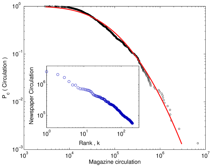
Figure 2: Cumulative distribution function of the 740 most circulated magazines in UK, fit by a log-normal curve (in red). The inset shows the rank-ordered plot of the top 200 newspapers in USA according to circulation.

II.1.5 Movies.

Movie popularity can be measured in a variety of ways, e.g., by looking at the votes given by users of various movie-related online forums. One of the largest of such forums is the Internet Movie Database (IMDb)  that allows registered users to rate films (and television shows) in the range 1-10 (with 1 corresponding to “awful” and 10 as “excellent”). We looked at the cumulative distribution of all votes received by movies or TV series shown between 2000-2004 (Fig. 3). The tail of the distribution approximately fits a log-normal distribution, with maximum likelihood estimates of the corresponding parameters, $\mu=8.60$ and $\sigma=1.09$. Next, we look at the distribution of average rating given to these items. As the minimum and maximum ratings that an item can receive are 1 and 10, respectively, this distribution is necessarily bounded. The skewed probability distribution of the average rating resulting from our analysis is shown in Fig. 3 (inset).

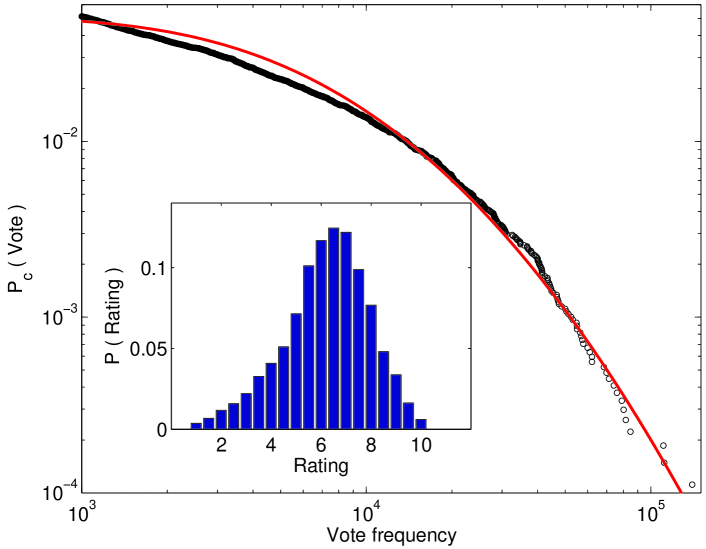
Figure 3: Cumulative probability distribution of the number of votes given by registered users of IMDb to movies and TV series released or shown between the years 2000-2004, fit by a log-normal curve (in red). (Inset) The probability distribution of the IMDb rating of a movie, averaged over all the votes received.

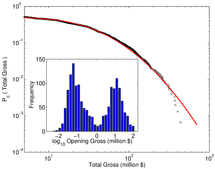
Figure 4: Cumulative distribution of total gross income for movies released across theaters in USA during 2000-2004, fit by a log-normal curve (in red). The inset shows the distribution of movie income according to the opening weekend gross.

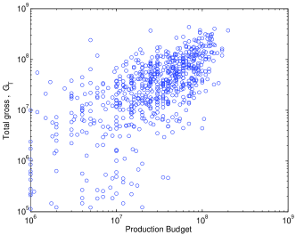
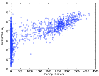
Figure 5: (Left) The total gross ($G_{T}$, in dollars) of a movie vs its production budget (in dollars). (Right) The total gross ($G_{T}$, in dollars) of a movie vs the number of theaters it is released on the opening weekend.

The measures used above have many drawbacks as indicators of movie popularity, particularly so when they are aggregated to produce average values. For example, users may judge different movies according to very different information, with so-called classic movies faring very differently from recently released movies that have very little information available about them. Also, it does not cost anything to vote for a movie, so that the vital element of competition among movies to become popular is missing in this measure. In contrast, looking at the gross income distribution of movies that are being shown at theaters gives a sense of the relative popularity of movies that have roughly equal amount of information available about them. Also, this kind of “voting with one’s wallet” is a truer indicator of the viewer’s movie preferences. The freely available datasets about weekly earnings of most movies released across theaters in the USA makes this a practical exercise. For our study we have concentrated on data from The Movie Times  and The Numbers  websites for the period 2000-2004. Although total gross may be a better measure of movie popularity, the opening gross is often thought to signal the success of a particular movie. This is supported by the observation that about 65-70 $\%$ of all movies earn their maximum box-office revenue in the first week of release De Vany and Walls (1999). The rank-ordered distribution for the opening, as well as the total gross, show an approximate power law with an exponent $1/\alpha\sim-1/2$ in the region where the top grossing movies are located Sinha and Raghavendra (2004a). However, when the data are aggregated together we find that the distribution (Fig. 4) is better fit by a log-normal  (similar to the observation of Redner vis-a-vis citations) Pan and Sinha (2006). The maximum likelihood estimates of the log-normal distribution parameters yield $\mu=3.49$ and $\sigma=1.00$. Further, we observe that the total gross distribution is just a scaled version of the opening distribution, which essentially implies that the popularity distribution of movies is decided at the opening itself. An additional feature of interest is that both the opening and the total gross distributions are bimodal (Fig. 4, inset), implying that most movies either do very well or very badly at the box office.

We have tried to see whether the popularity of individual movies correlate with its production quality (as measured by production budget). Fig. 5 (left) shows a plot of the total gross vs production budget for a large number of movies released between 2000-04 whose budget exceeded $10^{6}$ $. As is clear from the figure, although in general, movies with higher production budget tend to earn more, there is no significant correlation (the correlation coefficient is only 0.62). One can also argue that the determination of success of a movie on its opening implies the key role of pre-release advertising. Although the data for advertising budget is often unavailable, we can use as a surrogate, the data about the number of theaters that a movie is initially released at, since the advertising cost will scale with this quantity. As is obvious from Fig. 5 (right), the correlation here is worse, indicating that advertising has often very little role to play in deciding the success or otherwise of a movie in becoming popular. In this context, one may note that De Vany & Walls have looked at the distribution of movie earnings and profit as a function of a variety of variables, such as, genre, ratings, presence of stars, etc. and have not found any of these to be significant determinants De Vany (2003).

To make a quantitative analysis of the relative performance of movies, we have defined the persistence time $\tau$ of a movie as the time (measured in number of weekends) upto which it is being shown at theaters. We observe that most movies run for upto about 10 weekends, after which there is a steep drop in their survival probability. The empirical data seem to fit a Weibull distribution quite well.

II.1.6 Websites and Blogs

Zipf’s law for the distribution of requests for pages from the web was first reported by Glassman Glassman (1994). By tracing web accesses from DEC’s Palo Alto facilities, $~{}10^{5}$ HTTP requests were gathered and the rank-ordered distribution of pages was shown to have an exponent $\sim-1$. This was supported by a popular article Nielsen (1997) which observed Zipf’s law when analysing the incoming page-requests to a single site (www.sun.com). However, subsequent investigation of the page request distribution seen by web proxy caches using traces from a variety of sources, found the rank-order exponent to vary between 0.64 to 0.83 Breslau et al. (1999). The deviation from the earlier result (showing exact Zipf’s law) was ascribed to the fact that web accesses at a web server and those at a web proxy are different, because the former includes requests from all users on the Internet while the latter includes only those users from a fixed group. Access statistics for web pages have also been analysed by Adamic and Huberman from the access logs of about 60000 individual usage logs from America Online Adamic and Huberman (2000). The resulting cumulative distribution of website popularity, according to the number of unique visits to a website by users, showed a power law fit with $\alpha$ very close to 1.

Another obvious measure of webpage popularity is the number of links to it from another webpage. Distribution of incoming links to a webpage (i.e., URLs pointing to a certain HTML document) for the nd.edu domain, have been shown to obey a power law with exponent $\simeq-2.1$ Albert et al. (1999). This power law was quantitatively confirmed (i.e., the same exponent value of 2.1 was reported) over a much larger data set involving a web-crawl on the entire WWW with $2\times 10^{8}$ webpages and $1.5\times 10^{9}$ links Broder et al. (2000). While the power law distribution of popularity of websites according to the number of incoming links has been well-established as a power law, among web-pages of the same type (e.g., the set of US newspaper homepages) the bulk of the distribution of incoming links deviates strongly from a power law, exhibiting a roughly log-normal shape Pennock et al. (2002).

The finding that the micro-structure of popularity within a group is closer to a log-normal distribution has created some controversy among researchers involved in measuring the popularity distribution of blogs  which have over the past few years picked up a large following all over the web. Shirky Shirky (2003) had arranged 433 weblogs in rank order according to number of incoming links from other blogs and had claimed an approximate power law distribution. In contrast to this, Drezner & Farrell Drezner and Farrell (2004) conducted a study of the incoming link distribution of over 4000 blogs dealing almost exclusively with political topics, and found the distribution to be much better fit by a log-normal than a power law. Other studies have made contradictory claims about whether the popularity of blogs is better fit by a log-normal or power-law tailed distribution Hindman et al. (2002); Adamic and Glance (2005).

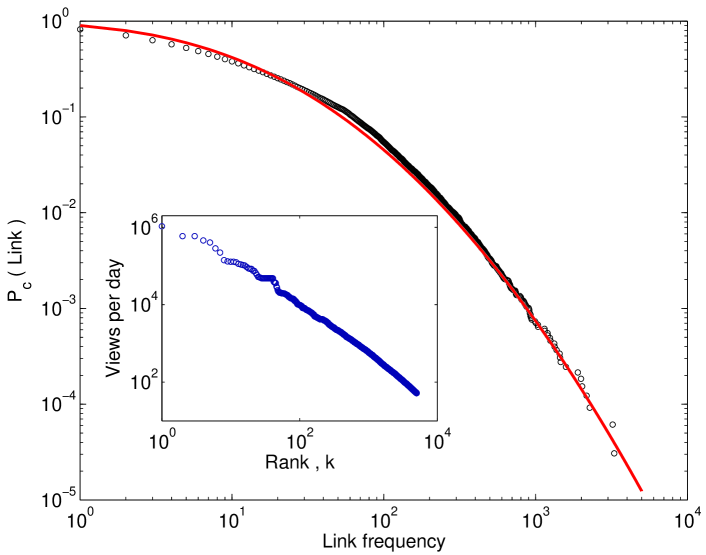
Figure 6: Cumulative distribution function for blog popularity measured by the number of incoming links a blog receives from other weblogs listed in the TTLB Blogosphere ecosystem within the past 7-10 days. The curve is the best log-normal fit to the data. The inset shows the rank-ordered plot of blog popularity according to the number of visits to a blog in a single day, in the TTLB ecosystem.

We have also analysed the popularity distribution of blogs according to citations in other blogs, using three different blogosphere ecologies, i.e., directories of blog listings. Such ecologies scan all blogs registered with them for (i) the number of links they receive from other blogs in their list, as well as (ii) the number of visits to that blog. These two measures of popularity complement each other, as the former looks at who is getting the most links from other bloggers, while the latter shows which blogs are actually receiving the most readers. The most extensive data that we have analyzed comes from the TTLB Blogosphere ecosystem  that lists 52048 blogs. In Fig. 6 we show the CDF for the popularity of blogs from this ecology, measured from the number of links to that blog seen in the “front page” of other member blogs within the past 7-10 days. This can be considered a rolling snapshot of the relative popularity of different blogs at a particular instant of time. For comparison, we also looked at data from two other ecologies, namely, the Technorati  and the Blogstreet  ecosystems, and observed qualitatively almost identical behavior. The CDF (Fig. 6) shows an approximately log-normal fit; maximum likelihood estimates of parameters for the corresponding distribution are $\mu=1.98$ and $\sigma=1.51$. We have also analyzed the popularity of blogs listed in the TTLB ecosystem according to traffic, i.e., views per day (Fig. 6, inset), which shows a power law over almost two decades for the rank-ordered plot. The maximum likelihood estimate of the corresponding exponent for the cumulative probability density yields $\alpha\sim 0.67$.

II.1.7 File Downloads.

Another web-related measure of popularity is that of file downloads. There are numerous file repositories in the net which allow visitors to download files either freely or for a fee. We focussed on files stored in the MATLAB Central File Exchange , which are computer programs. We looked at the number of downloads of all files over a period of one month during early 2006. The CDF [Fig. 7 (left)] shows an approximately log-normal fit; maximum likelihood estimates of parameters for the corresponding distribution are $\mu=3.76$ and $\sigma=0.89$.

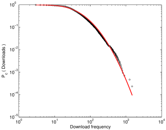
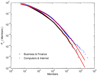
Figure 7: (Left) Cumulative distribution function for the number of downloads of different files in 1 month during early 2006 from the MATLAB file exchange site. (Right) Cumulative distribution function for the number of members in different Yahoo groups under the Business & Finance (squares) and Computers & Internet (diamonds) categories. Groups with less then 5 members are not considered. For both figures, the curves (in red) are the best log-normal fits to the data.

II.1.8 Groups.

A fertile area for observing the distribution of popularity is in the arena of social groups. While the membership of clubs, gangs, co-operatives, secret societies, etc., are difficult to come by, with the rising popularity of the internet it is easy to obtain data for online communities such as those in Yahoo  or Orkut . By observing the memberships of each of the groups in the community that a user can join, one can have a quantitative measure of the popularity of these groups. An analysis of the Yahoo groups resulted in a fat-tailed cumulative distribution of the group size Noh et al. (2005). Even though the distribution has a significant curvature over the entire range, the tail fits a power law for slightly more than a decade, with exponent $\alpha=1.8$.

We have recently carried out a smaller-scale study of the popularity of Yahoo groups . As in the earlier study, the popularity of the groups in each category has been estimated by the number of group members. Fig. 7 (right) looks at the cumulative distributions of the group size for two categories, namely Business & Finance and Computer & Internet, which comprise 182086 and 172731 groups respectively. However, unlike the power-law reported in the earlier study, we found both the distributions to approximately fit a log-normal form, with the parameters for the corresponding distributions being $\mu=2.80$, $\sigma=2.00$ and $\mu=3.10$, $\sigma=2.05$, respectively.

One can also look at the popularity of individual members of an online group, which has been analysed for a different type of community in the web: that formed by the users of the Pretty-Good-Privacy (PGP) encryption algorithm. To ensure that identities are not forged, users certify one another by “signing” the other person’s public encryption key. In this manner, a directed network (the “web of trust”) is created where the vertices are users and links are the user certifications. A measure of popularity in this case will be the number of certifications received by an user from other users, i.e., the number of incoming links for a vertex in the “web of trust”. The in-degree cumulative distribution has been reported to be a power law with the exponent $\alpha\simeq 1.8$ Guardiola et al. (2002).

II.1.9 Elections.

Political elections are processes that can be viewed as contests of popularity between individual candidates, as well as parties. The fraction of votes received by candidates is a direct measure of their popularity, regardless of whether the electoral system uses a majority voting rule (where the candidate with the largest number of votes wins) or a proportional representation (parties getting representation at the legislative house proportional to their fraction of the popular vote). Such studies have been carried out for, e.g., the 1998 Brazilian general elections Filho et al. (1999), which looked at the fraction of votes received by candidates for the positions of state deputies. The resulting frequency distribution was fit by a power law with exponent very close to $-1$. The cumulative distribution, however, revealed that about $90\%$ of the candidates’ votes followed a log-normal distribution, with a large dispersion that resulted in the apparent power law.

Figure 8: Canadian elections: (Left) The rank-ordered plot of candidate popularity measured by the fraction of votes received by him or her, for four successive general elections. The inset shows the cumulative frequency distribution function for this popularity measure. Note the region of linear decay in the middle of the curve. (Right) Cumulative probability distribution function for the fraction of votes received by a candidate for all constituencies in the 2000 general election. The inset shows the cumulative distribution function of the vote fraction for candidates for all polling booths at each constituency in the above election. Note that a constituency can have hundreds of polling booths.

We have carried out an analysis of the distribution of votes for a number of general elections in Canada and India. The data about votes for individual candidates in Canada was obtained from the website Elections Canada On-line  for the general elections held in 1997, 2000, 2004 and 2006. The total number of candidates in each election varied between 1600-1800, there were over $\sim 300$ electoral constituencies and the total number of votes cast varied around 13 million. Each constituency was divided into hundreds of polling stations, thereby allowing us to obtain a micro-level picture of the popularity of the candidates at a particular constituency across the different polling stations. Fig. 8 (left) shows the results of our analysis, indicating an exponential decay of the tail of the popularity distribution for all the elections being considered. The results don’t change even if we consider the number of votes, rather than the vote fraction. Fig. 8 (right) shows that the distribution of popularity across polling stations has almost an identical distribution to that seen over the larger scale of electoral constituencies. Note that we did not observe the popularity of parties for Canada, as the total number of parties were only about 10.

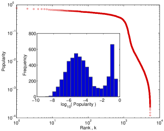
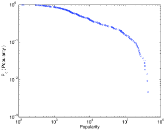
Figure 9: Indian election: (Left) The rank-ordered plot of candidate popularity measured by the fraction of votes received, for the 2004 Lok Sabha election. The inset shows the frequency distribution of the vote fraction, clearly indicating a bimodal nature with candidates receiving either most of the votes cast or very few. (Right) Cumulative probability distribution function of party popularity for the 2004 election, measured by the fraction of votes received by candidates from that party, over all the constituencies it contested in.

Next, we looked at the corresponding data for the 2004 general elections in India obtained from the website of the Election Commission of India . The total number of candidates is 5435, about half of whom belonged to 230 registered parties, who contested from a total of 543 electoral constituencies, while the total number of votes cast was about 400 million. Fig. 9 (left) shows that the rank-ordered popularity (measured by the vote fraction) distribution for candidates in an Indian general election is qualitatively similar to that of Canada, except for the presence of a kink indicative of the bimodal nature of the distribution. This implies that candidates either receive most of the votes cast by electors in that constituency or very few votes. It maybe due to the very large number of independent candidates (i.e., without affiliation to any recognized party) in Indian elections compared to Canada. This is supported by our analysis of popularity of recognized political parties [Fig. 9 (right)] that shows an exponential decay at the tail. Note that the popularity of a party is measured by the total votes received by a party divided by the number of constituencies in which it contested. This is same (upto a scaling constant) as the percentage of votes received by candidates belonging to a party, averaged over all the constituencies in which the party had fielded candidates.

II.1.10 Books.

An obvious popularity distribution based on product sales is that of books, especially in view of the record-breaking sales in recent times of the Harry Potter series of books. However, the lack of freely available data about exact sales figures has so far prevented detailed analysis of book popularity. It was reported in a recent paper Sornette et al. (2004), that the cumulative distribution of book sales from the online bookseller Amazon  has a power-law tail with $\alpha\sim 2$. However, one should note that Amazon does not reveal exact sales figures, but rather only the rank according to sales; therefore, this distribution was actually based on a heuristic relation between rank and sales proposed by Rosenthal Rosenthal (2004). Needless to say, this is at best a very rough guide to the exact sales figures (e.g., although the sale of Harry Potter and the Half-Blood Prince fluctuated a lot during the few weeks following its publication, it remained steady as the top ranked book in Amazon) and is likely to yield misleading distribution of sales. A more reliable dataset, if somewhat old, has been compiled by Hackett Hackett (1967) for the total number of copies sold in USA of the top 633 bestselling books between 1895 and 1965. Newman Newman (2005) has reported the maximum likelihood estimate for the exponent of the power law fit to this data as $\alpha\sim 2.51$. Fig. 10 (left) shows the rank-ordered plot of this data, indicating an approximate power law fit for slightly more than a decade, with an exponent of $-0.4$.

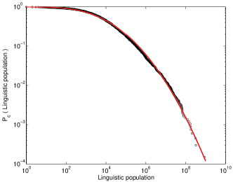
Figure 10: (Left) The rank-ordered plot of bestselling books (that sold 2 million copies or more) according to the number of copies sold in USA between 1895 to 1965. Adapted from Ref. Newman (2005), data provided by M. E. J. Newman. (Right) Cumulative distribution function for the size of the population of first-language speakers for over 6650 languages. The data was obtained from Ethnologue. The curve (in red) indicates the best log-normal fit to the data.

II.1.11 Language.

Fig. 10 (right) shows the cumulative distribution of the first-language speaker population for different languages around the world. The data has been obtained from Ethnologue  which provides the number of first-language speakers (over all countries in the world) wherever possible. Out of a total of 7299 languages listed in its 15th edition, we have considered above 6650 languages for which information about the number of speakers is available. The figure shows a long tail with an approximately log-normal fit; maximum likelihood estimates of parameters for the corresponding distribution are $\mu=8.78$ and $\sigma=3.17$. Note that this kind of popularity distribution is different from the others we have discussed so far as the speakers are not really free to choose their first language; rather this is connected to the population growth rate of a particular linguistic community. A similar kind of popularity distribution is that for family names, which has been analysed by Miyazima et al Miyazima et al. (1999) for Japanese family names and Newman Newman (2005) for American family names, both reporting cumulative distribution functions with power law tails having $\alpha$ close to 1. However, for Korean family names Kim and Park (2004) the distribution was reported to be exponentially decaying.

II.1.12 Other Popularity distributions.

Unlike the distribution of family names discussed above, the frequency of occurrence of given names (or first names) are indeed subject to waves of popularity, with certain names appearing to be very common at a particular period. A recent study Galbi (2005) has looked at the distribution of most popular given names in England and Wales over the past millennium, and has claimed a long-tailed distribution for the same. Another popularity distribution is that of tourist destinations, as measured by the number of tourist arrivals over a time period. A study Ulubasoglu and Hazari (2004) that has ranked 89 countries, focussing on the period 1980-1990, have found evidence for a log-normal distribution as the best fit to the data.

The occurrence of superstars (i.e., extremely successful performers) in popular music has led to a relatively large amount of literature by economists on the occurrence of popularity Rosen (1981); Adler (1985); MacDonald (1998); Hamlen (1994). Chung & Cox have used the number of gold-records by performers as the measure of their artistic success, and found the tail of this popularity distribution to approximately follow a power law Chung and Cox (1994). Another study Davies (2002) looked at the longevity of music bands in the list of Top 75 best-selling recordings, and observed a stretched exponential distribution . However, a more recent study Giles (2005) has shown the survival probability of a music recording on the Billboard Hot 100 chart to be fit better by the log-logistic distribution.

II.2 Time-evolution of popularity

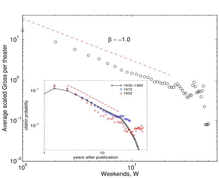
Figure 11: Weekend gross per theater for a movie (scaled by the average weekend gross over its theatrical lifespan), after it has run for $W$ weekends, averaged over the number of movies that ran for that long. The initial decline follows a power-law with exponent $\beta\simeq-1$ (the fit is shown by the broken line). The inset (from Ref. Redner (2004)) shows the probability that a paper will be cited $t$ years after publication in a Physical Review journal, in the years 1952 and 1972, as well as over the period 1932-1982. Over the range of $2-20$ years the integrated data is consistent with a power law decay having an exponent $-0.94$ (broken line in red).

Here we look briefly at how popularity evolves over time. For movies, we look at the gross income per theater over time (Fig. 11). This is a better measure of the dynamics of movie popularity than the time-evolution of the weekly overall gross income, because a movie that is being shown in a large number of theaters has a bigger income simply on account of higher accessibility for the potential audience. Unlike the overall gross that decays exponentially with time, the gross per theater shows a power-law decay in time with exponent $\beta\simeq-1$ Sinha and Pan (2005). This has a striking similarity with the time-evolution of popularity for scientific papers in terms of citations. It has been reported that the citation probability to a paper published $t$ years ago, decays approximately as $1/t$ Redner (2004) [Fig. 11 (inset)]. Note that, Price Price (1976) had also noted a similar behavior for the decay of citations to papers listed in the Science Citation Index. In a very different context, namely, the decay in the popularity of a website (as measured by the rate of download of papers from the site) over time $t$ has also been reported to follow an inverse power-law, but with a different exponent Johansen and Sornette (2000).

II.3 Discussion

The selection of (mostly) long-tailed empirical popularity distributions presented above underlines the following broad features of such distributions: (i) the entire distribution seem to be fit by a log-normal curve (in the few cases where the entire distribution is not available, the upper tail seems to fit a power law with characteristic exponent $\alpha$ which is often close to $1$, corresponding to the exact form of Zipf’s law); (ii) in some cases the distribution shows a bimodal character, with most of the instances occurring at the two ends of the distribution; (iii) the decay of popularity in some cases seem to show a simple power law decay, declining inversely with time elapsed since release; (iv) the persistence time at high levels of popularity show a Weibull distribution in many instances.

The first of these features may come somewhat as a surprise, because for many popularity distributions, power law tails have been reported with various exponents, often significantly different from 1. However, we observe that very often log-normal distributions have been mistakenly identified as having power law tails. In fact this is a very common error, especially if the variance of the log-normal distribution is sufficiently large. To see this, note that the log-normal distribution,

$$P(x)=\frac{1}{x\sigma\sqrt{2\pi}}e^{-({\rm ln}x-\mu)^{2}/2{\sigma}^{2}},$$ (5)

can be written as (on taking logarithm on both sides),

$${\rm ln}P(x)=-\frac{({\rm ln}x)^{2}}{2\sigma^{2}}+(\frac{\mu}{\sigma^{2}}-1)-{\rm ln}\sqrt{2\pi}\sigma-\frac{\mu^{2}}{2\sigma^{2}},$$ (6)

which is a quadratic curve in a doubly logarithmic plot. However, a sufficiently small part of the curve will appear as a straight line, with the slope depending on which segment of the curve one is focussing attention Newman (2005); Mitzenmacher (2003).This is the origin of most of the power law tails with exponent $\alpha\neq 1$ that has been reported in the literature on popularity distributions.

III Models of Popularity Distribution

From the perspective of physics, popularity can be viewed as an emergent outcome of the collective decision process in a society of individual agents exercising their free will (as reflected in their individual preferences) to choose between alternative products or ideas (Fig. 12). In a system without authoritarian control, agents differ in their personal preferences which are determined by the information available to the agent about the possible alternatives. However, in any real-life scenario with uneven access to information, a seemingly well-informed agent may influence the choice of several other agents Bikhchandani et al. (1992). Thus, the emergence of a popular product is a result of the self-organized coordination of choices made by heterogeneous entities.

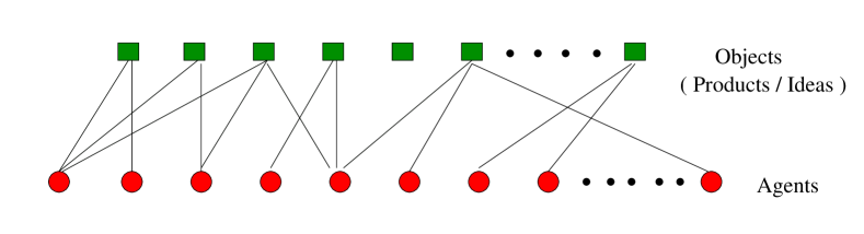
Figure 12: A schematic diagram of the emergence of popularity as a relation between agents and objects (products or ideas).

The simplest model of collective choice is one where the agents decide independently of each other and select alternatives at random with a one-step decision process. It is easy to see that the possible alternatives will not be significantly different in terms of popularity from each other. In particular, the popularity distribution arising from such a process will not have long tails. There are two possible alternative modifications of this simple model that will allow it to generate distributions similar to the ones seen empirically. The first option is to allow interactions between agents where the choice of one agent can influence that of another. While this is often true in real-life, we also observe long-tailed distributions much before the interaction among agents (and the resulting dissemination of information) has had a chance to influence the popularity. For example, the long-tailed distribution of movie popularity, in terms of gross earning, is seen at the opening weekend itself, long before potential movie viewers have had a chance to be influenced by other moviegoers. The second option for generating realistic popularity distribution gets around this problem: here we replace the single-step decision process by one comprising of multiple sub-decisions (as there may be many factors involved in making a particular decision), each of which contribute to the overall decision to purchase a particular product. Therefore, the probability of any particular entity achieving a particular degree of popularity can be expressed as the product of probabilities of each of the underlying factors satisfying the required condition to make an agent opt for that entity. As is easily seen, the resultant distribution arising from such a multiplicative stochastic process has a log-normal form, agreeing with many of the empirically observed distributions .

While the bulk of the popularity distributions, showing a log-normal nature, can therefore be plausibly explained as the product of the multiplicative stochastic structure underlying even apparently simple decision processes, this would still leave unanswered the reason for the wide occurrence of Zipf’s law in other instances. We now turn to the first option for extending the simple model outlined above, i.e., investigating the influence of an agent’s choice behavior on other agents. It turns out there have been many proposed mechanisms to explain the ubiquity of power-law tailed distributions employing interactions. However, from the point of view of the present paper, the most relevant (and general) model seems to be the Yule process Yule (1925), as modified by Simon Simon (1955). This is essentially a cumulative advantage process by which the relatively more popular entities get even more popular by virtue of being more well-known.

The Yule-Simon process can be described as follows: Suppose initially there are $n$ agents, each of whom are free to choose one of a number of products. Subsequently, the number of agents is augmented by unity at each time step. At any point in time, when the total number of agents is $m$, the number of distinct products, each of which have been chosen by $k$ agents is denoted by $f(k,m)$. Then, given that, (i) there is a constant probability, $\gamma$, that an agent chooses a completely new product (i.e., one that has not been chosen before by any of the agents) and (ii) the probability of choosing a product that has already been chosen by $k$ agents is proportional to $kf(k,n)$, one obtains an asymptotic popularity distribution that has a power-law tail  with exponent $\alpha=\frac{1}{1-\gamma}$. If the appearance of a new product is relatively infrequent, i.e., $\gamma$ is extremely small, then the exponent $\alpha\simeq 1$ (i.e., Zipf’s law).

Another feature of popularity distributions that has been mentioned earlier is that, in some cases, they appear to have a bimodal nature. We now present a simple agent-based model Sinha and Raghavendra (2004b) that shows how bimodal and unimodal distributions of popularity can arise very simply through agents interacting with each other, and reacting to information about what the majority are choosing in the previous time step.

III.1 A Model for Bimodal Distribution of Collective Choice

We have already discussed the simplest model of collective choice in which individual agents make completely independent decisions. For binary choice (i.e., each agent can only choose between two options) the emergence of collective choice is equivalent to a one-dimensional random walk with the number of steps equal to the number of agents. Therefore, the outcome will be normally distributed, with the most probable outcome being an equal number of agents choosing each alternative. While such unimodal distributions of popularity are indeed observed in some situations, as mentioned earlier in this article many real-life examples show the occurrence of bimodal distributions indicative of highly polarized choice behavior among agents resulting in the emergence of a highly popular product. This polarization suggests that agents not only opt for certain choices based on their personal preferences, but are also influenced by other agents in their social neighborhood. Also, the personal preferences may themselves change over time as a result of the outcome of previous choices, e.g., whether or not their choice agreed with that of the majority. This latter effect is an example of global feedback process that we think is crucial in the occurrence of bimodal behavior.

We now present a general model of collective decision that shows how polarization in the presence of individual choice volatility can be achieved with an adaptation and learning dynamics of the personal preference. In this model, the choice of individual agents are not only affected by those of their neighbors, but, in addition, their preference is modified by their previous choice as well as information about how successful their previous choice behavior was in coordinating with that of the majority. Here it is assumed that information about the intrinsic quality of the alternative products is inaccessible to the agent, who takes the cue from what the majority is choosing to decide which one is the “better choice”. Examples of such limited global information about the majority’s preference available to an agent are the results of consumer surveys and publicity campaigns disseminated through the mass media.

The simplest, binary choice version of our model is defined as follows. Consider a population of $N$ agents, each of whom can be in one of two choice states $S=\pm 1$ (e.g., to buy or not to buy a certain product, to vote Party A or Party B, etc.). In addition, each agent has an individual preference, $\theta$, that is chosen from a uniform random distribution initially. At each time step, every agent considers the average choice of its neighbors at the previous instant, and if this exceeds its personal preference, makes the same choice; otherwise, it makes the opposite choice. Then, for the $i$-th agent, the choice dynamics is described by:

$$S_{i}^{t+1}={\rm sign}(\sum_{j\in{\cal N}}J_{ij}S_{j}^{t}-\theta_{i}^{t}),$$ (7)

where sign ($x$) = $+1$, if $x>0$, and = $-1$, otherwise. The coupling coefficient among agents, $J_{ij}$, is assumed to be a constant ($=1$) for simplicity and normalized by $z$ ($=|{\cal N}|$), the number of neighbors. In a lattice, ${\cal N}$ is the set of spatial nearest neighbors and $z$ is the coordination number, while in the mean field approximation, ${\cal N}$ is the set of all other agents in the system and $z=N-1$.

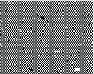
Figure 13: (Left) The spatial pattern of choice ($S$) in the absence of learning ($\lambda=0$) in a two-dimensional square lattice of $1000\times 1000$ agents after 500 iterations starting from a random configuration. The figure is a magnified view of the the central $100\times 100$ region showing the absence of long-range correlation among the agents. (Right) The spatial pattern of choice ($S$) with learning ($\lambda=0.05$) in the same system, with a majority of agents now in the choice state $S=+1$. The magnified view of the central $100\times 100$ region shows coarsening of regions having agents aligned in the same choice state.

The individual preference, $\theta$, evolves over time as:

$$\theta_{i}^{t+1} = \theta_{i}^{t}+\mu S_{i}^{t+1}+\lambda S_{i}^{t},~{}{\rm if}~{}S_{i}^{t}\neq{\rm sign}(M^{t}),$$ (8)

$$= \theta_{i}^{t}+\mu S_{i}^{t+1},{\rm otherwise},$$

where $M^{t}=(1/N)\sum_{j}S_{j}^{t}$ is the collective decision of the entire community at time $t$. Adjustment to previous choice is governed by the adaptation rate $\mu$ in the second term on the right-hand side of Eq. (8), while the third term, governed by the learning rate $\lambda$, represents the correction when the individual choice does not agree with that of the majority at the previous instant. The desirability of a particular choice is assumed to be related to the fraction of the community choosing it; hence, at any given time, every agent is trying to coordinate its choice with that of the majority. Note that, for $\mu=0,\lambda=0$, the model reduces to the well-known zero-temperature, random field Ising model (RFIM).

Random neighbor and mean field model. For mathematical convenience, we choose the $z$ neighbors of an agent at random from the $N-1$ other agents in the system. We also assume this randomness to be “annealed”, i.e., the next time the same agent interacts with $z$ other agents, they are chosen at random anew. Thus, by ignoring spatial correlations, a mean field approximation is achieved.

For $z=N-1$, i.e., when every agent has the information about the entire system, it is easy to see that, in the absence of learning ($\lambda=0$), the collective decision $M$ follows the evolution equation rule: $M^{t+1}={\rm sign}[(1-\mu)M^{t}-\mu\sum_{\tau=1}^{t-1}M^{\tau}].$ For $0<\mu<1$, the system alternates between the ordered states $M=\pm 1$ with a period $\sim 4/\mu$. The residence time at any one state ($\sim 2/\mu$) diverges with decreasing $\mu$, and for $\mu=0$, the system remains fixed at one of the ordered states corresponding to $M=\pm 1$, as expected from RFIM results. At $\mu=1$, the system remains in the disordered state, so that $M=0$. Therefore, we see a transition from a bimodal distribution of the collective decision, $M$, with peaks at non-zero values, to an unimodal distribution of $M$ centered about 0, at $\mu_{c}=1$. When we introduce learning, so that $\lambda>0$, the agents try to coordinate with each other and at the limit $\lambda\rightarrow\infty$ it is easy to see that $S_{i}={\rm sign}(M)$ for all $i$, so that all the agents make identical choice.In the simulations, we note that the bimodal distribution is recovered for $\mu=1$ when $\lambda\geq 1$.

For finite values of $z$, the population is no longer “well-mixed” and the mean-field approximation becomes less accurate the lower $z$ is. For $z<<N$, the critical value of $\mu$ at which the transition from a bimodal to a unimodal distribution occurs in the absence of learning, $\mu_{c}<1$. For example, $\mu_{c}=0$ for $z=2$, while it is 3/4 for $z=4$. As $z$ increases $\mu_{c}$ quickly converges to the mean-field value, $\mu_{c}=1$. On introducing learning ($\lambda>0$) for $\mu>\mu_{c}$, we again notice a transition to an ordered state, with more and more agents coordinating their choice.

$Lattice.$ To implement the model when the neighbors are spatially related, we consider $d$-dimensional lattices ($d=1,2,3$) and study the dynamics numerically. We report results obtained in systems with absorbing boundary conditions; using periodic boundary conditions leads to minor changes but the overall qualitative results remain the same. It is worth noting that the adaptation term disrupts the ordering expected from results of the RFIM for $d=3$, so that for any non-zero $\mu$ the system is in a disordered state when $\lambda=0$.

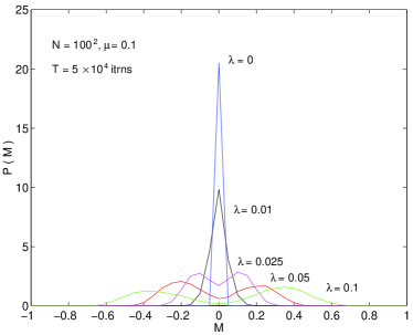
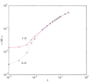
Figure 14: (Left) The probability distribution of the collective decision $M$ in a two-dimensional square lattice of $100\times 100$ agents. The adaptation rate $\mu=0.1$, and the learning rate $\lambda$ is increased from 0 to 0.1 to show the transition from unimodal to bimodal behavior. The system was simulated for $5\times 10^{4}$ iterations to obtain the distribution. (Right) The order parameter $<|M|>$ for one- and two-dimensional lattices. The adaptation rate is $\mu=0.1$, while $\lambda$ is increased gradually to show the transition to an ordered state. Note that for higher values of $\mu$ the two curves are virtually identical. There is very little system size-dependence of the curves.

In the absence of learning ($\lambda=0$), starting from a initial random distribution of choices and personal preferences, we observe only very small clusters of similar choice behavior [Fig. 13 (left)] and the average choice $M$ fluctuates around 0. In other words, at any given time an equal number (on average) of agents have opposite choice preferences. Introduction of learning in the model ($\lambda>0$) gives rise to significant clustering as well as a non-zero value for the collective choice $M$. We find that the probability distribution of $M$ [Fig. 14 (left)] evolves from a single peak at 0, to a bimodal distribution as $\lambda$ increases from 0. This is similar to second-order phase transition in systems undergoing qualitative changes at a critical threshold. The collective decision $M$ switches periodically from a positive value to a negative value having an average residence time which diverges with $\lambda$ and with $N$. For $\mu>\lambda>0$, large clusters of agents with identical choice are observed to form and dissipate throughout the lattice [Fig. 13 (right)]. After sufficiently long times, we observe the emergence of structured patterns having the symmetry of the underlying lattice, with the behavior of agents belonging to a particular structure being highly correlated. Note that these patterns are dynamic, being essentially concentric waves that emerge at the center and travel to the boundary of the region, which continually expands until it meets another such pattern. Where two patterns meet their progress is arrested and their common boundary resembles a dislocation line. In the asymptotic limit, several such patterns fill up the entire system. These patterns indicate the growth of clusters with strictly correlated choice behavior. The central site in these clusters act as the “opinion leader” for the entire group. This can be seen as analogous to the formation of “cultural groups” with shared preferences Axelrod (1997). It is of interest to note that distributing $\lambda$ from a random distribution among the agents disrupts the symmetry of the patterns, but we still observe patterns of correlated choice behavior. It is the global feedback ($\lambda\neq 0$) which determines the formation of large connected regions of agents having similar choice behavior. This is reflected in the order parameter, $\langle|M|\rangle$, where $\langle\cdots\rangle$ indicates time averaging. Fig. 14 (right) shows the order parameter increasing with $\lambda$ in both one and two dimensional lattices, signifying the transition from a disordered state to an ordered state, where neighboring agents have coordinated their choices.

Our model seems to provide an explanation for the observed bimodality in a large number of social or economic phenomena, e.g., in the distribution of the gross income for movies released in theaters across the USA during the period 1997-2003 Sinha and Raghavendra (2004a). Bimodality in this context implies that movies either achieve enormous success or are dismal box-office failures. Based on the model presented here, we conclude that, in such a situation the moviegoers’ choice depends not only on their neighbors’ choice, but also on how well previous action based on such neighborhood information agreed with media reports and reviews of movies indicating the overall or community choice. Hence, the case of $\lambda>0$, indicating the reliance of an individual agent on the aggregate information, imposes correlation among agent choice across the community which leads to a bimodal gross distribution.

Based on a study of the rank distribution of movie earnings according to their ratings De Vany and Walls (2002), we further speculate that movies made for children (rated G) have a significantly different popularity mechanism than those made for older audiences (PG, PG-13 and R). The former show striking similarity with the rank distribution curve obtained for $\lambda=0$, while the latter are closer to the curves corresponding to $\lambda>0$. This agrees with the intuitive notion that children are more likely to base their choices about movies (or other products, such as toys) on the choice of their friends or classmates, while adults are more likely to be swayed by reports in mass media about the popular appeal of a movie. This suggests that one can tailor marketing strategies to different segments of the population depending on the role that global feedback plays in their decisions. Products whose target market has $\lambda=0$ can be better disseminated through distributing free samples in neighborhoods; while for $\lambda>0$, a mass media campaign blitz will be more effective.

IV Conclusions

In this article we have primarily made an attempt to ascertain the general empirical features inherent in many popularity phenomena. We observe that the distribution of popularity in various contexts often exhibit long tails, the nature of which seem to be either following a log-normal form or a power law with the exponent $\alpha\simeq 1$ (Zipf’s law). While the log-normal distribution would arise naturally in any multiplicative stochastic process, in the context of popularity it would be natural to interpret it as a manifestation of the interplay of the multiple factors involved in an agent making a decision to adopt a particular product or idea. Further, there is no necessity for interactions among agents for this particular distribution in popularity to be observed. On the other hand, distributions with power law tails would seem to necessarily entail inter-agent interactions, e.g., a process whereby agents follow the choice of other agents, with a particular choice becoming more preferable if many more agents opt for it . This is not necessarily an irrational “herding” effect; for example, in the case of popularity of cities, the larger the population of a city, the more likely it is to attract migrants, owing to the larger variety of employment opportunities. Thus the very fact that more agents have chosen a particular alternative may make that choice more preferable than others. Seen in this light, the popularity distribution should show a log-normal distribution in situations where individual quality preferences play an important role in making a choice, while, in cases where the choice of other agents is a paramount influence in the decision process of an agent, Zipf’s law should emerge . In either case, a stochastic process is sufficient to generate the popularity distributions seen in reality. This suggests that the emergence of popularity can be explained entirely as an outcome of a sequence of chance events.