[0704.2993] A large scale extinction map of the Galactic Anticenter from 2MASS

\beginpicture

\setcoordinatesystem

units ¡-1.25984252mm,1.25984252mm¿ point at 179.5 0 \setplotareax from 243 to 116 , y from -32 to 31

The correct determination of extinction from colour excess methods requires that we remove the foreground stars to the cloud and that we reject young stellar objects. Both types of objects systematically influence the determined extinction values. Foreground stars lead to on average bluer colours, hence the extinction is underestimated. Young stars are intrinsically red and hence lead to an overestimate of the extinction. Due to the large range of distances of the clouds in our map (ranging from 140 pc to at least 1 kpc) the removal of foreground stars is very difficult. In principle the number of foreground stars has to be evaluated for each individual cloud and removed statistically. The large number of clouds in the map with partly unknown distances, or overlapping clouds close to the Galactic Plane makes this an almost impossible task. However, if the stars in each box are not dominated by foreground objects and one uses the median colour of stars instead of the average, then the foreground stars are removed automatically. Froebrich & del Burgo 2006MNRAS.369.1901F (2006) have shown (see their Fig. 9) that such an approach indeed reproduces the intrinsic extinction values of clouds extremely well, as long as the cloud is not too distant, or has a very high extinction. For very distant clouds or very high extinction regions, however, this approach detects zero extinction. Hence, locally more sophisticated procedures such as described in Lombardi 2005A&A…438..169L (2005) or suggested in Froebrich & del Burgo 2006MNRAS.369.1901F (2006) have to be used to obtain correct extinction values for the highest extinction regions. Since only a very small portion of the map area is affected and we are investigating only the large scale distribution of clouds and their properties in this paper, the main conclusions of this paper are not significantly changed by this effect. However, when using the presented extinction map one has to keep in mind that the extinction values in the very dense regions of clouds are underestimated and that there is a small $A_{V}$ dilution for more distant clouds. Similarly to the removal of foreground stars, the use of the median colour also removes intrinsically red YSOs, as long as they do not dominate (as e.g. in the Orion Nebula cluster).

\beginpicture

\setcoordinatesystem

units ¡-1.25984252mm,1.25984252mm¿ point at 179.5 0 \setplotareax from 243 to 116 , y from -32 to 31

The resulting $\left<J-H\right>$ and $\left<H-K\right>$ colour excess maps are converted separately into H-band extinction maps using Equ. 8 and 9 of Froebrich & del Burgo 2006MNRAS.369.1901F (2006), respectively. A power law index of the reddening law of $\beta$ = 1.73 is applied (see Sect. 2 for details). The resulting two H-band extinction maps are averaged and converted into our final optical extinction map by $A_{V}$ = 5.689 $\times$ $A_{H}$ , using the reddening law from Mathis 1990ARA&A..28…37M (1990). In Fig. LABEL:ext_map we show this map in gray-scale. Indicated in this figure are the regions of which we show magnified versions of the extinction map in Appendix A.1. These are also the regions we analyse in detail in the forthcoming sections. The full resolution FITS version of our entire map will be provided as online material to this paper. Note that the construction of the final extinction maps as average of the $A_{H}$ extinction maps from $\left<J-H\right>$ and $\left<H-K\right>$ colour excess maps leads to further dilution of the very high extinction cores. This will, however, effect the same areas that are dominated by foreground stars, as described above. Thus, the number of high column density regions in our analysis will be underestimated.

The noise in the extinction map can in principle only be measured in extinction free regions as the standard deviation of extinction values from zero. To estimate the noise in all areas we have determined a noise map (see Fig. LABEL:noisemap). Since we used the median colour of stars in each pixel, we need to determine the standard error of the median for our noise map. For a large sample and normal distribution this can in principle be done by $\sigma_{med}$ = $1.25\cdot\sigma/\sqrt{N}$ , where $\sigma$ is the error of the colour of the individual stars and $N$ the number of stars in each box. Since we use stars of different photometric quality (see below) and we do not know if the sample of stars in each pixel follows a normal distribution, we cannot use this equation. However, the fraction of stars for any given photometric quality is very constant (see below). Thus, we can conclude that the noise in each pixel is proportional to $1/\sqrt{N}$ for both, the $\left<J-H\right>$ and $\left<H-K\right>$ maps. We have thus scaled and co-added the $1/\sqrt{N}$ maps of stars with (J and H) and (H and K) photometry, in order to obtain the final noise map. The scaling was done to match the measured noise in the $A_{V}$ map in extinction free regions. As can be seen, the noise in the map varies significantly with Galactic Latitude, as well as with extinction. The 3 $\sigma$ noise ranges from 0.36 mag optical extinction, close to the Galactic Plane, to 1.0 mag $A_{V}$ in the most northern and southern parts of the map as well as in high extinction regions. In Table 1 we list for all individual regions the average number of stars with detections in J and H, as well as the average noise in the area. There are pixels in the map (0.0066 %) where the noise is extremely large, i.e, there are no stars to determine the colour. These regions are: 1) around very bright stars; 2) at $|b|>30^{\circ}$ ; 3) high extinction cores in Orion, Taurus, Perseus. For Ori A we determine an average noise of 0.24 mag, which can be compared to the 1 $\sigma$ noise level of about 0.2 mag $A_{V}$ obtained by Lombardi & Alves 2001A&A…377.1023L (2001) (see their Fig. 6) in this region using the optimised NICER method.

There are further areas in the map where the extinction values are not very reliable. These are positions close to dense star clusters. Here, the high number of stars in the cluster dominates the extinction determination. Hence, depending on the colour of the cluster members we measure either a too low (mostly blue stars) or too high (mostly young, red stars) extinction. Since this is a common effect, we over plotted circles at the positions of all known star clusters (found in SIMBAD) in the gray scale maps of our selected regions in Appendix A.1. Additionally we over plot $+$ signs at the positions of all possible new star clusters with $|b|<20^{\circ}$ found by Froebrich et al. 2006MNRAS.subm.F (2007).

Does the use of 2MASS quality BCD stars instead of only quality A stars influence the noise in our map? Independent of the position about 40–45 % of all stars are of quality AAA. Given the larger errors in photometry for the quality BCD objects, one can estimate that the noise in the extinction map is about 10 % (i.e. 0.03 mag) higher, when including the lower quality objects. However, as has been pointed out by Froebrich & del Burgo 2006MNRAS.369.1901F (2006), systematic errors of extinction determinations based on colour excess methods can be much higher than this, since the population of stars seen through a cloud can differ from the population of stars in a control field (even if close-by). The more than twice as large number of stars per resolution element when including the lower quality objects will lead to a much better representation of the population of stars and, as a result, to smaller systematic errors. This out weights in our opinion the slightly higher resulting statistical noise in our maps and justifies the use of the lower quality 2MASS sources.

Note that the galaxies M 31 ( $l$ =121.2, $b$ =-21.6) and M 33 ( $l$ =133.6, $b$ =-31.3) show up as apparently high extinction regions. In M 31 the structure in our extinction map resembles quite closely the 170 $\mu$ m emission map from Haas et al. 1998A&A…338L..33H (1998) and in particular we are able to identify the dominant ring of material in the disc of the Andromeda Galaxy.

Table 1: Names and areas of our individual regions, average numbers of stars in the 4’ x 4’ box, average noise in the field, peak in the distribution of

\beta

, intrinsic scatter of the

\beta

distribution, probability that the measured distribution is in agreement with the predicted one for the assumption of a constant

\beta_{0}

value and intrinsic scatter in the whole region and slope of the column density distribution in the logN vs.

A_{V}

plot.

ID	Name	$l$ -range	$b$ -range	$\#$ stars/box	$\sigma_{A_{V}}$ [mag]	$\beta_{0}$	$\sigma_{\beta_{intr}}$ [mag]	P [%]	slope
1	Auriga 1	156 – 173	$-$ 12 – $-$ 03	47	0.15	1.99	0.45	98.5	-0.68
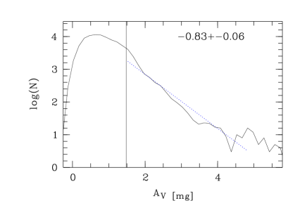
2	Auriga 2	175 – 186	$-$ 11 – $-$ 02	53	0.14	2.05	0.39	99.9	-0.83
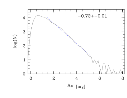
3	Cassiopeia	116 – 127	$-$ 04 – $+$ 10	90	0.11	1.67	0.43	99.9	-0.72
4	Camelopardalis 1	127 – 148	$+$ 03 – $+$ 15	53	0.15	1.96	0.49	98.4	-0.91
5	Camelopardalis 2	137 – 152	$-$ 05 – $+$ 04	78	0.12	1.40	0.54	98.5	-0.71
6	Camelopardalis 3	152 – 161	$-$ 04 – $+$ 08	74	0.12	1.66	0.49	95.2	-1.20
7	$\lambda$ -Ori	188 – 201	$-$ 18 – $-$ 06	36	0.18	1.87	0.24	96.3	-0.81
8	Monoceros	212 – 227	$-$ 13 – $+$ 01	67	0.14	1.52	0.53	82.7	-0.68
9	Orion B	201 – 211	$-$ 17 – $-$ 08	34	0.18	1.77	0.41	91.2	-0.38
10	Orion A	208 – 219	$-$ 21 – $-$ 16	20	0.24	1.66	0.59	99.8	-0.28
11	Perseus	156 – 163	$-$ 25 – $-$ 15	18	0.25	1.97	0.51	99.9	-0.30
12	Taurus	164 – 178	$-$ 19 – $-$ 10	27	0.20	1.99	0.47	99.9	-0.32
13	Taurusextended	171 – 189	$-$ 31 – $-$ 17	14	0.29	1.92	0.43	99.9	-0.49
14	Entire Field	116 – 243	$-$ 32 – $+$ 31	—	—	1.73	0.52	98.9	—

2 The Reddening Law

The conversion of colour excess maps into extinction maps requires the knowledge of the extinction law. Our approach of using $\left<J-H\right>$ and $\left<H-K\right>$ colour excess maps enables us to determine the power law index of the extinction law using the colour excess ratio $R$ $\equiv$ $\left<J-H\right>$ / $\left<H-K\right>$ and

0=\left(\frac{\lambda_{2}}{\lambda_{1}}\right)^{\beta}+R\cdot\left(\frac{\lambda_{3}}{\lambda_{2}}\right)^{-\beta}-R-1

(1)

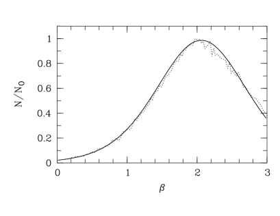
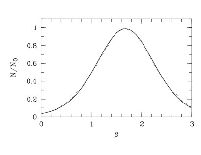
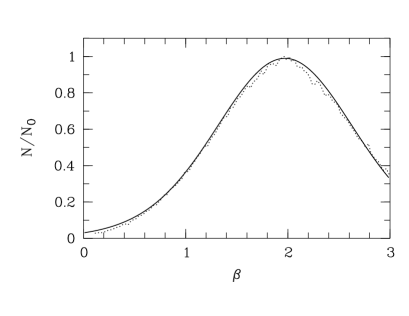
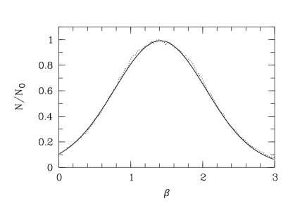
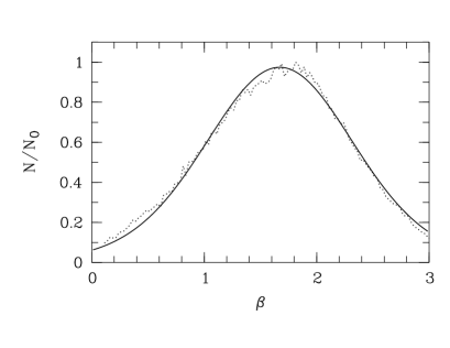
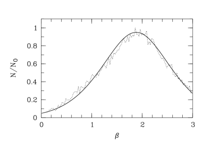
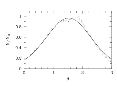
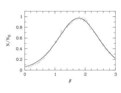
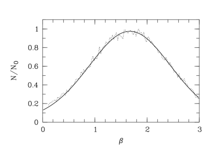
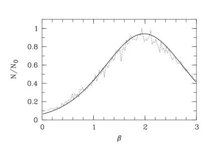
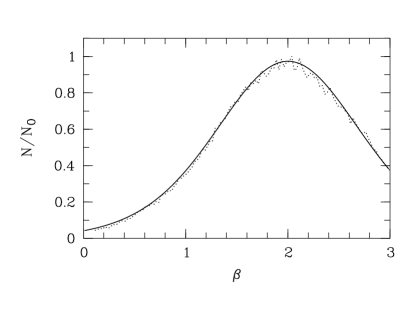
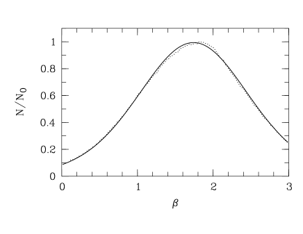
from Froebrich & del Burgo 2006MNRAS.369.1901F (2006). We now can analyse the resulting distribution of $\beta$ values in our maps. For all the following analysis of $\beta$ we use only areas where both, the $\left<J-H\right>$ and $\left<H-K\right>$ colour excess values are 3 $\sigma$ above the noise. In Fig. 1 we show the histogram of the measured distribution of all $\beta$ values ( $N_{o}(\beta)$ ) as dotted line. It peaks at 1.73, in good agreement with the canonical value for the interstellar medium (Draine 2003ARA&A..41..241D (2003)). We hence use $\beta$ = 1.73 to convert our colour excess maps into extinction. The distribution of $\beta$ values shows a rather broad peak with a FWHM of 1.6. This, seemingly, rather large value is in good agreement for the predicted scatter of about $\pm$ 40 % when using the colour excess ratio to determine $\beta$ (see e.g. Fig. 1 in Froebrich & del Burgo 2006MNRAS.369.1901F (2006)).

It is possible to investigate in more detail, if the measured distribution of $\beta$ values $N_{0}(\beta)$ is in agreement with a single value of $\beta_{0}$ =1.73 in the entire field or not. This can be done by convolving the observed distribution of signal to noise values, $N_{o}(\left<J-H\right>)$ , in our extinction map from Fig. LABEL:ext_map with the predictions for the width of the distribution of $\beta$ . We have, however, to allow for the possibility that there is an intrinsic scatter in the $\beta$ values ( $\sigma^{2}_{\beta_{int}}$ ) around $\beta_{0}$ . We hence have to adapt Equ. 11 from Froebrich & del Burgo 2006MNRAS.369.1901F (2006) and obtain:

\sigma^{2}_{\beta}=\frac{\sigma^{2}_{\left<\lambda_{1}-\lambda_{2}\right>}}{\left<\lambda_{1}-\lambda_{2}\right>^{2}}R^{2}\left[1+\frac{R^{2}}{\alpha_{\rm co}}-2\frac{R}{\gamma_{\rm co}}\right]\left(\frac{\partial{\bf B}(R)}{\partial R}\right)^{2}+\sigma^{2}_{\beta_{int}}

(2)

To determine the predicted distribution of $\beta$ values we use:

N_{p}(\beta)=N_{0}\int N_{o}(\left<J-H\right>)\cdot e^{-\frac{1}{2}\left(\frac{\beta-\beta_{0}}{\sigma_{\beta}(\left<J-H\right>)}\right)^{2}}\cdot d\left<J-H\right>

(3)

were $N_{0}$ is a normalisation factor and $\beta_{0}=1.73$ the peak of the measured $\beta$ distribution. A Kolmogorov Smirnov test can then be performed with $N_{o}(\beta)$ and $N_{p}(\beta)$ to determine the probability ( $P$ ) that the two distributions are drawn from the same sample.

In order to determine the predicted $\beta$ distribution we require to estimate the parameters $\alpha_{co}$ and $\gamma_{co}$ . The parameter $\alpha_{co}$ represents the square of the ratio of the noise in the two colour excess maps and $\gamma_{co}$ represents the ratio of the square of the noise in one colour excess map and the covariance of the two colour excess maps (see Equ. 2 and Froebrich & del Burgo 2006MNRAS.369.1901F (2006) for details). For our dataset we measure values of: $\alpha_{co}$ =3.6 and $\gamma_{co}$ =3.7. Note that the values for both parameters might slightly vary with position or hence from cloud to cloud. However, we have measured here the same values for $\alpha_{co}$ and $\gamma_{co}$ as were obtained for 2MASS data in IC 1396 W by Froebrich & del Burgo 2006MNRAS.369.1901F (2006). Due to this fact, and since the dependence of the predicted $\beta$ distribution on $\alpha_{co}$ and $\gamma_{co}$ is rather weak, we fix these values for all our determinations.

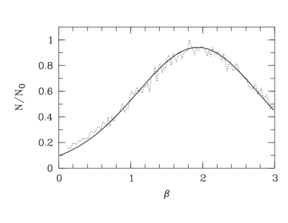
This gives us the possibility to vary the intrinsic scatter $\sigma^{2}_{\beta_{int}}$ and the $\beta_{0}$ value until we find the highest probability $P$ that the observed and predicted distributions of $\beta$ values match. We list the obtained values of those parameters as well as the probabilities for the individual regions in Table 1.

We over plot the resulting best predicted distribution for $\beta$ values of the entire field as solid line in Fig. 1. We find that with a 98.9 % probability the two distributions are equal, when a value of $\beta_{0}=1.73$ and an intrinsic scatter of $\sigma^{2}_{\beta_{int}}=0.52$ is assumed. The large intrinsic scatter shows, that there is a good chance that indeed variable $\beta$ values are present in different parts of the field. Hence, repeating the same analysis for selected regions should lead to different $\beta$ values in different clouds. If locally those clouds have more uniform dust properties, then a lower intrinsic scatter should be found.

Thus, similar to the entire area, we investigate the peak value of the $\beta$ distribution, the intrinsic scatter and how well the distribution matches the assumption of a constant $\beta$ value for our individual regions. In Table 1 we summarise the obtained results. We find an average value of $\beta$ = 1.8 $\pm$ 0.2. Almost in all investigated regions the $\beta$ value is in agreement with the estimate for the entire field. Only in Auriga 2 ( $\beta$ =2.05), Monoceros ( $\beta$ =1.52) and Camelopardalis 2 ( $\beta$ =1.40) significantly different values are found, hinting to different dust properties such as the grain size distribution in these areas. Notably, regions with smaller $\beta$ values tend to be closer to the Galactic Plane. However, it is not clear if this is caused by different dust properties or by the overlap of clouds in this area. Furthermore, small systematic off-sets in either $\left<J-H\right>$ or $\left<H-K\right>$ can cause changes in the determined $\beta$ value. Thus, the procedure of fitting a polynomial to the extinction free regions in order to determine the colour excess maps might also contribute to these smaller $\beta$ values. Since very close to the Galactic Plane there are no extinction free regions, the procedure might have introduced a small off-set in the colour excess maps and hence to the $\beta$ values. Clearly, more detailed investigations are required to find the cause of the smaller $\beta$ values very close to the Galactic plane.

We also find that for most regions the intrinsic scatter of the $\beta$ values is smaller or in the order of the value for the entire field. Only in Ori A is a significantly larger value found. The probabilities that measured and predicted values are drawn from the same sample are listed in Table 1 and the individual distributions are shown in Appendix LABEL:app_plots. We find that in some regions the proposal of constant $\beta$ values with the corresponding internal scatter is more probable than in others. Especially in the regions Monoceros and Ori B low probabilities ( $P<95\,\%$ ) are found. We can conclude that in these regions we do not see a dominant fraction of the dust possessing constant optical properties. This might indicate large scale variations of the optical dust properties within these clouds.

Refer to caption — Figure 1: Histogram of the distribution of $\beta$ values in the entire field (dotted line) measured for all pixels where the $\left<J-H\right>$ and $\left<H-K\right>$ colour excess values are at least 3 $\sigma$ above the noise. The solid line represents the predicted distribution for a value of $\beta$ =1.73, $\sigma_{\beta_{intr}}$ =0.52 and the measured distribution of $A_{V}$ values in the entire field (see text for details). A Kolmogorov Smirnov test shows that both distributions are identical with a probability of 98.9 %.

3 The Column Density Distribution

In order to analyse and interpret the distribution of column density values in the entire map, as well as in the individual regions, we first have to recapitulate the selection effects induced by our method. As outlined in detail in Sect. LABEL:extinction, our method of determining the extinction maps leads to three biases. (1) Very distant clouds, as well as very high extinction regions will not be detected by our method, since these areas are dominated by foreground stars. (2) There is a small $A_{V}$ dilution with distance. (3) The averaging of extinction maps from $\left<J-H\right>$ and $\left<H-K\right>$ colour excess maps leads to dilution of the high extinction cores. (4) Regions close to rich star clusters will be dominated by the colours of the cluster members. However, due to the use of the median stellar colours instead of the mean colours, all not too distant clouds without rich clusters and extremely dense cores, will have no systematically influenced extinction values.

The general way of analysing the structure of molecular clouds is to determine the distribution of clumps within them. This includes the clump mass, size and column density distribution. We have hence used the $clumpfind$ -2D algorithm (Williams et al. 1994ApJ…428..693W (1994)) to extract all detectable clumps in our final extinction map and determined their size and mass distribution. Contrary to line or dust emission maps, extinction maps have real, very smooth large scale profiles which make it very difficult to extract structure information using an automated thresholding technique. This is reflected by the fact that the determined clump properties from our map depended, partly significantly, on the chosen levels and also on the pixel size of the map.

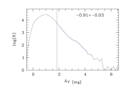
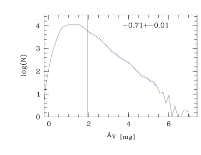
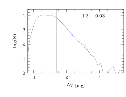
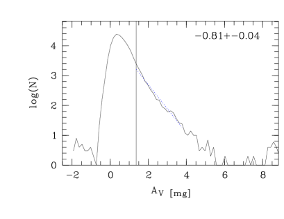
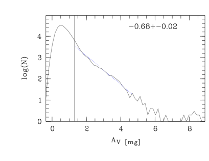
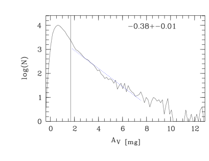
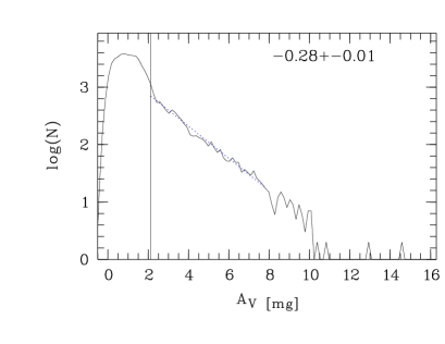
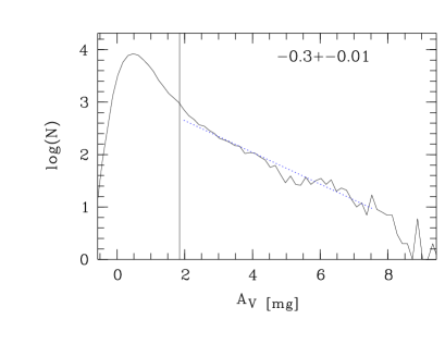
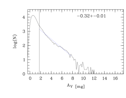
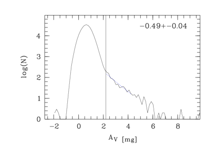
Hence, instead of using the clump properties in the map, we will analyse the column density distribution in the individual regions. Since the distance of the clouds will influence the measured slope of the column density distribution (see below), we will not analyse the distribution of the entire map as a whole. We show in Appendix LABEL:app_plots the $A_{V}$ distributions for all individual regions (solid line). For each region we fit a linear polynomial to the log(N) vs. $A_{V}$ plots (dashed line) for extinction values larger than the 5 $\sigma$ noise (vertical line). The measured slopes are indicated in the individual diagrams as well as in Table 1.

The individual $A_{V}$ distributions nicely show the above discussed biases for high extinction values. Some show a clear drop-off for regions with very high column densities. Depending on the distance of the cloud and its position, this drop-off occurs at different values. For Ori A and Ori B we see a clear drop at $A_{V}$ = 10 mag, while for Perseus ( $A_{V}$ = 8 mag) and Camelopardalis 2 ( $A_{V}$ = 6 mag) lower values are found. The values of the slopes range from about -0.3 to almost -1.0, with the exception of Camelopardalis 3 where -1.2 is found.

The interpretation of these values is, however, rather difficult. Two effects could influence the measured slope: (1) the distance of the cloud; (2) the intrinsic distribution of material. The distance could influence the slope since in more distant clouds the extinction per resolution element is averaged over a larger physical area in the cloud. Hence, for more distant clouds the column density distribution on larger physical scales is measured. One can artificially move a cloud to larger distances by using a larger box-size for the extinction measurements. Indeed one finds that this results in a steeper column density distribution. This is in agreement with the values obtained from our data, where more distant clouds possess on average steeper column density distributions. We basically find that in all clouds where our resolution element is smaller than 1 pc the slope of the distribution is -0.3. For all clouds were we are not able to resolve 1 pc (cloud distance larger than 850 pc) the slope in the column density distribution is about -0.75. This leads to the conclusion that there might be a change in the governing physics determining the column density distribution in molecular clouds on a scale of about 1 pc. Interestingly, this is about the Jeans length for a column density that is required for self-shielding and molecular hydrogen formation in molecular clouds (Hartmann et al. 2001ApJ…562..852H (2001)). The already discussed small $A_{V}$ dilution with distance could as well contribute to the change in the slope. Furthermore, there could also be intrinsic differences between clouds, as reflected by the different slopes measured for e.g. Ori A and Ori B, which are believed to be at the same distance. We note however, that if measured only for $b<-13^{\circ}$ the slope for Ori B is -0.32, hence in very good agreement with Ori A and the other close-by clouds Taurus and Perseus. For the region with $b>-13^{\circ}$ in Ori B the slope is -0.75, indicating that these clouds are more distant. We further note that an overlap of different clouds, as may happen close to the Galactic plane, does not change the measured slope if the individual clouds are at about the same distance and have intrinsically the same slope.

4 Conclusions

Using Grid technology and 2MASS data we created the largest extinction map to date based on near infrared colour excess. Our 127 ${}^{\circ}\times 63^{\circ}$ sized map of the Galactic Anticenter contains the molecular cloud complexes of Orion, Taurus, Cepheus, Monoceros, Auriga, Camelopardalis and Cassiopeia. The three sigma noise level ranges from 0.36 mag optical extinction close to the Galactic Plane to 1.0 mag $A_{V}$ at $|b|\approx 30^{\circ}$ and in high extinction regions. Our final optical extinction map has a resolution of 4’ and a pixel size of 2’.

The colour excess ratio $\left<J-H\right>$ / $\left<H-K\right>$ is used to determine the power law index $\beta$ of the wavelength dependence of the extinction in the near infrared. In the entire field the distribution of $\beta$ peaks at a value of 1.73. The average value of the investigated cloud complexes is determined to $\beta=1.8\pm 0.2$ . Both values are in agreement with the assumed values for the interstellar medium. We analyse in detail the distribution of $\beta$ values in the entire field and individual regions. It is found that there is an internal scatter in the $\beta$ values of about 0.4 – 0.5. A comparison of the measured and predicted $\beta$ distribution by means of a Kolmogorov Smirnov tests shows that in most regions the proposal of a constant $\beta$ with an internal scatter is valid. In some regions (e.g. Monoceros, Ori B) low probabilities that observations and predictions match are found. Hence, there is no dominant $\beta$ value in the cloud, a clear indication of large scale variations of the optical dust properties in these areas.

We further analysed the column density distribution of the individual regions. Due to our technique, the highest extinction cores ( $A_{V}>$ 10 mag) cannot be identified reliably. For extinction values up to 10 mag $A_{V}$ we find that the column density distributions show a linear behavior in the log(N) vs. $A_{V}$ plot. On average a steeper column density distribution for more distant clouds is found, i.e. the $A_{V}$ distribution is steeper when measured on larger spatial scales. This seems to indicate a change in the governing physics of the column density at scales of about 1 pc or an $A_{V}$ dilution with distance in our map.

acknowledgments

We are grateful to the anonymous referee for helpful comments which significantly improved the paper. We would like to thank D. O’Callaghan and S. Childs for very helpful discussions on Grid computing. D.F. and G.C.M received funding by the Cosmo Grid project, funded by the Program for Research in Third Level Institutions under the National Development Plan and with assistance from the European Regional Development Fund. This publication makes use of data products from the Two Micron All Sky Survey, which is a joint project of the University of Massachusetts and the Infrared Processing and Analysis Center/California Institute of Technology, funded by the National Aeronautics and Space Administration and the National Science Foundation. This research has made use of the SIMBAD database, operated at CDS, Strasbourg, France.

References

(1) Bok, B.J. 1956, AJ, 61, 309
(2) Coghlan, B.A., Walsh, J. & D. O’Callaghan 2005, in ’Advances in Grid Computing - EGC 2005’, Peter M.A. Sloot, Alfons G. Hoekstra, Thierry Priol, Alexander Reinefeld, and Marian Bubak, editors, LNCS3470, Amsterdam, The Netherlands, February 2005. Springer.
(3) Draine, B.T. 2003, ARA&A, 41, 241
(4) Froebrich, D., Scholz, A. & Raftery, C.L. 2007, MNRAS, 374, 399
(5) Froebrich, D. & del Burgo, C. 2006, MNRAS, 369, 1901
(6) Froebrich, D., Ray, T.P., Murphy, G.C. & Scholz, A. 2005, A&A, 432, 67
(7) Haas, M., Lemke, D., Stickel, M., Hippelein, H., Kunkel, M., Herbstmeier, U. & Mattila, K. 1998, A&A, 338, 33
(8) Hartmann, L., Ballesteros-Paredes, J. & Bergin, E.A. 2001, ApJ, 562, 852
(9) Lada, C.J., Lada, E.A., Clemens, D.P. & Bally, J. 1994, ApJ, 429, 694
(10) Lombardi, M. 2005, A&A, 438, 169
(11) Lombardi, M. & Alves, J. 2001, A&A, 377, 1023
(12) Mathis, J.S. 1990, ARA&A, 28, 37
(13) Padoan, P., Nordlund, A. & Jones, B.J.T. 1997, MNRAS, 288, 145
(14) Skrutskie, M.F., Cutri, R.M., Stiening, R., et al. 2006, AJ, 131, 1163
(15) Williams, J.P., de Geus, E,J. & Blitz, L. 1994, ApJ, 428, 693
(16) Wolf, M. 1923, AN, 219, 109

Appendix A Individual Regions

A.1 Extinction and $\beta$ maps

In the following we show for all individual regions investigated in this paper larger versions of the extinction and $\beta$ maps. Note that the full resolution FITS file of the extinction map is provided as online material to the paper. We overplot in the maps the position of all known star clusters in the field found in SIMBAD (circles) as well as the new star cluster candidates ( $+$ signs) found in Froebrich et al. 2006MNRAS.subm.F (2007), in order to mark regions were potentially the cluster members might dominate the extinction determination (see Sect. LABEL:extinction for details).