Mass Loss and Evolution of Stars and Star Clusters:
a Personal Historical Perspective

Abstract

The development and progress of the studies of winds and mass loss from hot stars, from about 1965 up to now, is discussed in a personal historical perspective. The present state of knowledge about stellar winds, based on papers presented at this workshop, is described. About ten years ago the mechanisms of the winds were reasonably well understood, the mass loss rates were known, and the predictions of stellar evolution theory with mass loss agreed with observations. However, recent studies especially those based on $FUSE$ observations, have resulted in a significant reduction of the mass loss rates, that disagrees with predictions from radiation driven wind models. The situation is discussed and future studies that can clarify the situation are suggested. I also discuss what is known about the dissolution of star clusters in different environments. The dissolution time can be derived from the mass and age distributions of cluster samples. The resulting dissolution times of clusters in the solar neighborhood (SN) and in interacting galaxies are shorter than predicted by two-body relaxation of clusters in a tidal field. Encounters with giant molecular clouds can explain the fate of clusters in the SN and are the most likely cause of the short lifetime of clusters in interacting galaxies.

Astronomical Institute, Utrecht University, Princetonplein 5, 3584-CC Utrecht, The Netherlands

1. Introduction

In this final talk of the workshop I want to take you back about 40 years and show you the progress of ideas in the two main topics of this conference: mass loss and evolution of stars and of star clusters. I will show you that many ideas that are now taken for granted came as a surprise when the technological progress opened up new possibilities. I will start at about 1965, when I became involved in astronomical research . (Excellent reviews of the more recent situation have been written by Kudritzki & Puls, 2000 and by Puls et al., these proceedings, astro-ph/0607290)

2. Massive Hot Stars: Dull and Not Interesting

In the 1950s and 1960s massive hot stars did not get much attention. They were rather dull compared to cool stars and their properties were well understood (or at least that was the general feeling).
- They did not have chromospheres.
- They were not variable (apart from the Beta Cepheid stars).
- Their optical spectrum showed relatively few spectral lines, mainly of simple ions.
- They all had the same abundances.

Of course, not everything was understood. There were some puzzling spectral features:
- Some of the brightest O-stars showed H$\alpha$ in emission, but this was probably just a non-LTE effect that was not yet properly understood.
- Some stars had stronger N and O lines than other stars, but this was probably also a non-LTE effect.
- There were some unidentified emission lines, but again these were probably due to some non-LTE effect.

Apart from the “normal” early type stars, there were also some special types of hot stars:
- The Be-stars showed emission lines in their optical spectrum, that suggested circumstellar disks. These stars were known to be fast rotators, so their disks were probably due to the centrifugal force.
- The Wolf-Rayet stars with their strong and broad emission lines were already known to have a stellar wind with a high velocity and high mass loss rate of order $10^{-5}$ $\mathit{M}_{\odot}{\rm yr}^{-1}$, as shown already in 1934 by Kosirev. However, some astronomers thought that these lines were due to a chromosphere and not to a wind.
- The pathological stars like $\eta$ Car, P Cygni and the like were known to have erupted, but the nature of these outbursts and the connection to other stars was unknown. They were simply strange exceptions.

In general, there was little interest in spectroscopic studies of early type stars, apart from their use as tracers of recent star formation. Most surprisingly, there was almost nothing known about the evolutionary connection between these different classes of hot stars!. For instance, my teacher Anne Underhill (1966), in her famous book “The early type stars” discussed the observations and properties of all kinds of early type stars but did not mention the possible evolutionary connections at all!

3. 1967 - 1976: The First UV Observations: All Luminous Early Type Stars have Mass Loss!

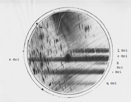
Figure 1.: The picture that changed our concept of the evolution of massive stars (Morton 1967a). The horizontal bands are the UV spectra of five bright stars in Orion: from top to bottom: $\zeta$, $\epsilon$ plus $\kappa$ partly overlapping, $\iota$ and $\eta$ Ori. Wavelength range approximately 1200 to 2000 Å, increasing to the right. The P Cygni profiles of Si iv and C iv can easily be seen. The small blotches are the first order images of Orion stars that were used for wavelength calibration.

This picture of rather dull hot stars changed drastically in the late 60s and early 70s after the first UV spectra were obtained. Morton (1967a) observed the UV spectra of Orion Belt stars with a camera in a stabilized nose-cone of an Aerobee rocket over White Sands. The resulting image (Fig. 1) is both awful and magnificent. It is awful because the flight failed for the second time and the camera with the photo-cassette made a hard landing and was found after two days of searching in the desert. There are stripes and blotches all over the picture. At the same time, it is beautiful because it showed for the first time the strong P Cygni profiles of UV resonance lines. Using a simple curve of growth analysis Morton (1967b) estimated mass loss rates of order $10^{-6}$ $\mathit{M}_{\odot}{\rm yr}^{-1}$ with outflow velocities of 1000 to 3000 ${\rm km\,sec^{-1}}$.

The mechanism for the strong stellar winds of hot supergiants was quickly identified as radiation pressure. Lucy and Solomon (1970) were the first to show that the strong UV resonance lines produce enough radiation pressure to counteract gravity and accelerate the wind to high velocity by their Doppler-shift.

Within a decade it was clear that mass loss was not limited to the OB supergiants. Mass loss from A-supergiants was discovered by the Utrecht UV spectrograph S59, aboard the European TD1a satellite. The near-UV spectrum of $\alpha$ Cyg showed strong and blue-shifted resonance lines of Mg ii with a velocity of only 200 ${\rm km\,sec^{-1}}$ (Lamers 1975).

Then the $Copernicus$ satellite was launched. Snow and Morton (1976) published the first catalog of P Cygni profiles which showed that basically all early type stars more luminous than $M_{\rm bol}=-6$ have winds, even the main sequence stars. These observations also showed that the winds of practically all early type stars were super-ionized, i.e. the degree of ionization was higher than could be expected on the basis of their effective temperature (see also Lamers & Snow, 1978). The high resolution spectra allowed the first detailed quantitative analysis of the P Cygni profiles, the first empirical wind model and the first accurate determination of the mass loss rates of the stars $\zeta$ Pup (O4If) (Lamers & Morton, 1976) and $\tau$ Sco (B0V) (Lamers & Rogerson, 1978). We suggested a simple velocity law, the $\beta$-law, and found evidence for the presence of strong “turbulence” in the winds. We found that the mass loss of $\zeta$ Pup could not be explained by the observed UV-lines only, but required the existence of many more lines in the far UV below 912 Å. This was predicted at about the same time by the radiation driven wind theory of Castor et al. (1975a).

The observations and the new theory showed that mass loss would affect the evolution of all massive stars! That was a very important conclusion that changed the ideas about massive stars drastically.

Within a few years three major steps in understanding the evolution of massive stars were taken:
- Castor et al. (1975b) pointed out that a massive star throughout its lifetime injects as much energy and mass into the ISM as a supernova. They also showed that the winds from hot stars blow bubbles and that star clusters blow superbubbles in the interstellar medium.
- Conti (1976) proposed a scenario that linked the different types of massive stars into an evolutionary sequence with mass loss, including the Luminous Blue Variables and the WR-stars: the “Conti scenario”.
- de Loore et al. (1977) in Brussels and Maeder (1980) in Geneva calculated the first evolution tracks of massive stars with mass loss.

4. 1975 - 1980: Stellar Winds studied in Different Wavelength Regions

Shortly after the discovery that all massive stars have winds there were many attempts to quantify the wind parameters, such as mass loss rate and velocity law. It was realized that this could be done using observations at different wavelength regions, which would probe different regions of the winds.

- Panagia & Felli (1975) showed that stars with ionized winds emit an excess radio emission, due to the free-free process, that could be used to derive the emission measure (EM) of the wind. Combined with information about the terminal velocity, derived from spectroscopic UV data, the mass loss rate could be derived. (This circumvented the difficult problem of the super-ionization of the stellar winds, which plagued the mass loss studies based on UV lines.) The radio flux originates far out in the wind where the wind velocity has reached a constant value. White & Becker (1982) later showed in their study of P Cygni that this model can be tested and the wind temperature can be derived if the radio image of the wind can be resolved.
- Barlow & Cohen (1977) showed that the winds also produce an infrared excess by free-free emission and derived mass loss rates from ground-based infrared observations. This emission is generated in the lower layers of the wind, where the acceleration takes place. So its interpretation in terms of mass loss rate requires an accurate knowledge of the density and velocity structure in the lower layers.
- Klein & Castor (1978) showed that mass loss rates can also be derived from the equivalent width of the H$\alpha$ and He ii emission lines. Again this requires knowledge of the density and velocity structure in the lower parts of the wind. This method was later used by Leitherer (1988) and Lamers & Leitherer (1993), who adopted the mass loss rates derived from the radio-flux to calibrate the H$\alpha$ rates.
- Cassinelli et al. (1978) pointed out that the super-ionization could be due to Auger-ionization by X-rays. They predicted that hot star winds are X-ray emitters.
- Vaiana et al. (1981) detected X-rays from OB supergiants with the Einstein satellite. The observed X-ray spectra were interpreted by Cassinelli et al. (1981) who showed that the source of the X-rays is distributed throughout the wind, as predicted by the shocked wind model of Lucy & White (1980).

5. 1975 - 1990: Development of Wind Theories

Already in 1975, at about the time the $Copernicus$ observations were made, Castor et al. (1975a) published their famous theory that the winds of hot stars can only be explained if they are driven by a mixture of optically thick and optically thin lines. This became known as the “CAK-theory”. It showed that the mass loss rate could be much higher than the limit of $N\times L/c^{2}$. (The limit for mass loss by one optically thick line at the peak of the Planck curve is about $\dot{M}\simeq L/c^{2}$ and the Copernicus observations showed that there are about $N\simeq 6$ strong wind lines in the UV spectrum at $\lambda>912$ Å.) The CAK theory was based on the Sobolev approximation and on the assumption of a “typical CNO-ion” for the calculation of the multitude of optically thick and thin lines. It proved successful in explaining the trends in observed mass loss rates and wind velocities.

When the Boulder wind group dissolved, the group of Kudritzki and colleagues in Munich took over the lead in the theories of stellar winds. They improved the CAK-theory in two major ways:
(1) they dropped the assumption of the star being a point source and took its finite disk into account (Kudritzki et al. 1989),
(2) they calculated the strength of an enormous number of lines ($\sim 10^{6}$) of many relevant ions (Pauldrach 1987).
As a result, their predicted mass loss rates and wind velocities agreed much better with observations than the older CAK-predictions.

Hydrodynamical models of stellar winds by Owocki et al. (1988) improved the original suggestion of Lucy & White (1980) that line driven winds are inherently unstable. Fortunately, these hydrodynamical models also showed that the mass loss rates and wind velocities predicted by the improved CAK theory were still correct because they are hardly affected by the presence of shocks.

6. 1990 - 2000: Everything fits nicely ! (apart from Some “Minor” Problems)

After the improvements of the observations and wind theories described above, the situation seemed rather satisfactorily in the 1990s:
- the basic properties of the winds were known,
- the basic mechanism was well understood,
- the predictions agreed nicely with the observations,
- evolution with mass loss could explain almost all observations.
Unfortunately there were two problems that did not seem to be solved: super-ionization and clumping.

6.1. Super-Ionization

The problem of super-ionization was first raised by the $Copernicus$ observations which showed strong spectral lines of high ionization species, such as O vi, O v, N v and N iv in the spectra of O-stars and lines of C iv and Si iv in stars down to spectral types B3 (Snow & Morton 1976, Lamers & Snow 1978). These stars are too cold to create these ions by photo-ionization due to stellar radiation.

Originally there were three suggested explanations:
- I proposed that the winds of O-stars were “warm”, with $T\sim 2~{}10^{5}$ K, in order to explain O vi by collisional ionization in a low density gas and not destroy C iv (Lamers & Morton 1976; Lamers 1979).
- Joe Cassinelli suggested that the super-ionization was due to Auger ionization. He suggested that hot stars had a thin corona low in the wind (Cassinelli et al. 1978).
- John Castor suggested a “tepid” wind of $T\sim 6~{}10^{4}$ K that was optically thick and produced the high ions by photo-ionization (Castor 1979).
When the X-rays from hot stars were discovered by the $Einstein$ satellite (Vaiana et al. 1981), Joe was proclaimed the winner!

However, it soon became clear that the source of the X-rays was distributed throughout the wind, i.e. due to shocks (Cassinelli et al. 1981). This made it difficult to model and explain the super-ionization because the models of shocked wind were (and still are) not good enough to predict the ionization fractions accurately.

The problem became even more severe when the $IUE$ satellite (1978-1996) observed the spectra of hundreds of early type stars, but only long-ward of 1215 Å. This excluded the lines of C iii, O vi, P v, S vi and S iv etc. that were observed with the Copernicus satellite and limited the mass loss tracers of hot stars effectively to N v, C iv and Si iv. To make things worse, the Si iv and C iv lines are often saturated and provide only a lower limit to the mass loss rates. The N v lines are usually not saturated, but they are from a trace ion that is sensitive to X-rays of an element whose abundance can change during the evolution of a star. The determination of the mass loss rate from these lines requires large and uncertain correction factors for its ionization fraction.

The general feeling was that the $FUSE$ satellite, to be launched in 1999, would solve this problem because it would observe the wavelength range down to the Lyman limit where the unsaturated P Cygni profiles could be observed, just as the $Copernicus$ satellite had done for a small number of stars. Some of these lines, especially S iv and S vi and P v, are from trace elements (i.e. the lines are not saturated) that are not affected by changes in the surface composition during the evolution of the massive stars (but see below).

6.2. Clumping

With the mass loss rates derived from UV lines being uncertain, the attention shifted to the emission lines in the optical spectrum, mainly H$\alpha$ (Klein & Castor 1978, Leitherer 1988, Puls et al. 1996). However, the detailed analysis of the H$\alpha$ profiles soon showed that the strength of the wings of these emission lines did not agree with the equivalent width (EW) of the emission (see e.g. Hillier 1991; Puls et al. these proceedings, astro-ph/0607290). The EW depends on the emission measure of the wind. On the other hand the wings of the emission lines depend on electron column density. Adopting a velocity law and using the corresponding density structure (these are coupled by the equation of mass continuity) the mass loss rates derived from the wings and from the EW should give the same mass loss rate. It turned out, however, that in many (most?) cases they don’t.

The mass loss rate derived from the EM is usually larger than that derived from the wings (Puls et al., these proceedings). This indicates that the lower layers of the wind, where most of the H$\alpha$ photons are created, is “clumpy”: the mean value $<n_{e}^{2}>$ is larger than the value of $<n_{e}>^{2}$. So obviously, the structure of the wind is uncertain, especially in the lower layers, and the determination of mass loss rates from H$\alpha$ profiles is not straightforward.

In principle the radioflux, which is also from free-free emission and hence depends on $n_{e}^{2}$, is also sensitive to clumping. However, the radioflux comes from far out in the wind and one might assume that the clumps or shocks due to instabilities deep in the wind have dissolved by the time the flow reaches a large distance. So the mass loss rates derived from the radio flux are considered to be the most reliable ones. Unfortunately the small flux limited the number of stars that were observed at radio wavelengths to the brightest ones with the highest mass loss rates (e.g. Abbott et al. 1980; Lamers & Leitherer 1993; review by Kudritzki & Puls 2000). With new and more sensitive radio telescopes this number may increase drastically.

7. 2000 - now: The state of Confusion

7.1. Structures in the Wind?

The last few days we heard many talks about mass loss rates, which together present a nice state-of-the-field review. What is my impression? The topic is even more uncertain than it was before!

- Observations of lines below 1250 Å by the $FUSE$ satellite, suggest that the mass loss rates are “much” lower than derived from the “standard” UV resonance lines by as much as as a factor 3 to 10. This would imply clumping factors of $f\simeq 10-100$.
- Part of the problem may be due to the fact that the Sobolev approximation is not strictly valid in the complicated winds of OB-stars. For instance, this is a basic assumption in the $SEI$ program that is used in several studies for calculating and fitting line profiles. The analysis of spectra with more modern methods, e.g. $FASTWIND$ by Puls et al. (2005), may give more accurate mass loss rates (e.g. Mokiem et al. 2006)
- Another part of the problem may be that clumping might affect the degree of ionization of the observed ions. The X-rays photons that are generated in the shocked wind will also affect the ionization. An overestimate of the assumed ionization fraction of an ion whose spectral lines have been measured, results in an underestimate of the mass loss rate and vice-versa. The trace ions of dominant elements are expected to be most sensitive to this effect.
- The clumping may be distance dependent. If that is the case, the rates derived from H$\alpha$, from the free-free excess in the IR and the radio regions will all be different. There is evidence that this is indeed the case for the star $\zeta$ Pup, which is the standard test star for mass loss, ever since the first analysis of its $Copernicus$ spectrum.
- Clumping might be different in different types of OB stars, e.g. the supergiants and the main sequence stars. This implies that even the relative mass loss rates and the trends of mass loss with stellar parameters are uncertain.

I wonder how much of this confusion is due to the fact that the winds may be far less spherically symmetric than is assumed in all studies so far.

Stellar atmosphere models that are used to derive the stellar parameters (which are input for the wind studies) and the wind models themselves are always assumed to be spherically symmetric. Even the most sophisticated wind models with distance dependent clumping factors and shocks are still assumed to be spherically symmetric. What if the wind is much more structured? If that is the case, the different lines of sight to the star through the wind might probe different wind structures. For instance, if some lines of sight to the stellar disk pass through very little wind material and others pass through the thick wind regions, the UV line profiles will be weakened by the contribution of continuum radiation from the lines of sight with low column densities. If spherical symmetry is assumed in the analysis of such a profile, the mass loss will be seriously underestimated.

Is there evidence for non-spherical winds? Certainly!
(1) The variable discrete absorption components that are modulated with the rotation period clearly show evidence that the wind has large non-spherical structures.
(2) Massive stars may be fast rotating. In this case, not only will the polar region be hotter than the equatorial regions (due to the von Zeipel effect), but the wind from the polar region may also be different from that of the equatorial regions, e.g. in terms of velocity, density, shocks, and ionization. In that case the lineprofiles will depend on the inclination angle to the star, which is usually unknown.

The challenge will be in the next few years to explain the clumping and confirm or deny the new low mass loss rates

7.2. Mass Loss versus Luminosity

In the last few years we have seen several papers pointing to the steep drop in mass loss rate of O-stars in the Magellanic Clouds at luminosity $\log L/L_{\odot}\lesssim 5$ (e.g. Martins et al. 2004). This is usually presented as a completely unexpected discovery. The reason that it was unexpected is probably because in recent years we have started to believe that the mass loss rates scale with luminosity as a power-law. This was predicted for OB-stars by the original CAK-theory and by newer predictions of Vink et al. (2000). Observed mass loss rates of supergiants and giants confirmed this trend.

It may be forgotten that the original mass loss observations with the $Copernicus$ satellite had already shown that, going down along the main sequence from early-O to late-B, the mass loss rate suddenly drops by an order of magnitude or more between about spectral type O9 and B0 (Snow & Morton 1976). In general, main-sequence stars later than B0 do not show mass loss signatures in their UV spectra, unless the star is rotating rapidly (Snow & Marlborough 1976). So, there seems to be a luminosity (?) limit for high mass loss rates $\dot{M}\geq 10^{-7}\,\mathit{M}_{\odot}{\rm yr}^{-1}$.

I wonder if the low mass loss rates of the O-main-sequence stars in the Magellanic Clouds maybe another manifestation of this same effect.

7.3. The Bistability Jump: Does it Exist ?

Pauldrach & Puls (1990) noted in their models of P Cygni that the structure of the wind changes drastically when they adopted two slightly different values for luminosity or radius. In one case the wind was much slower but the mass loss rate much higher than in the other case. For P Cyg this flip occurs around $\mathit{T}_{\rm eff}\simeq 19300$ K. They called this “bistability” because they argued that the star could jump from one solution to the other and back. It is due to the drastic change in the degree of ionization and in the lines that provide the radiation pressure for driving the wind, mainly metal lines.

Based on this idea, Lamers et al. (1995) measured $v_{\infty}$ of 68 supergiants in a homogeneous way and calculated the ratio $v_{\infty}/v_{\rm esc}$, because that ratio was predicted to depend on $\mathit{T}_{\rm eff}$ in the radiation driven wind models of CAK and the Munich group. We had to adopt a $\mathit{T}_{\rm eff}$ scale based on spectral type. We found that there was a strong jump in the ratio $v_{\infty}$/$v_{\rm esc}$ around supergiants of type B1 Ia. Not only the velocity was drastically different on either side of this type, but more importantly, so was the observed degree of ionization. The ratio of the line strength of C ii/C iii/C iv changed drastically over one spectral subtype, with a high C ii/C iv ratio corresponding to a low value of $v_{\infty}/v_{\rm esc}$ and vice-versa. We called it the “bistability jump”.

Vink et al. (1999) showed that the jump is due to the the change in ionization from Fe iv on the high-T side to Fe iii on the low-T side. Fe iii has a much larger number of optically thin lines than Fe IV, which results in a higher $\dot{M}$ and a lower $v_{\infty}$. (In terms of the CAK force multiplier parameters, $k$ increases and $\alpha$ decreases.) When $\mathit{T}_{\rm eff}$ of a star decreases due to stellar evolution and passes the jump temperature, then Fe goes from Fe iv to Fe iii. The resulting higher mass loss rate and smaller velocity produces an increase in wind density (because $\rho\sim\dot{M}/v$) which pushes the ionization even further down. This is a positive feedback that results in a change in $\dot{M}$ and $v_{\infty}$ in a narrow temperature region of $\Delta\mathit{T}_{\rm eff}\simeq 2000$ K “for any given star”.

Several groups have improved our study, using larger samples of stars and, importantly, also using better values of $\mathit{T}_{\rm eff}$ (e.g. Prinja & Massa 1998, Crowther et al., these proceedings, astro-ph/0606717). They find that the jump appears to be less steep then found in our original study, and that the changes occur over several spectral subtypes. They conclude that the wind structure changes much less rapidly with $\mathit{T}_{\rm eff}$ than we found. In my opinion, this last conclusion is due to a misunderstanding of the physical process that causes the change in the wind structure.

The temperature where this jump occurs depends on the stellar parameters, e.g. the luminosity, mass and radius. This can be understood easily. A star of higher $L/M$ ratio will have a higher mass loss rate and hence a higher wind density than a star with the same $\mathit{T}_{\rm eff}$ but a smaller $L/M$ ratio. This means that the degree of ionization in the first star will be lower and hence the jump from Fe iii to Fe iv will occur at a lower value of $\mathit{T}_{\rm eff}$ (see also Vink et al. 2000). The exact value of $\mathit{T}_{\rm eff}$ where the jump occurs will depend on $L$ and $M$ of a star. So it is no wonder that, as more and more stars of different $L/M$ ratios are plotted in a diagram of $v_{\infty}$ versus $\mathit{T}_{\rm eff}$, the jump will become more vague. This is not important. The important question is: how fast, i.e. within how small a $\mathit{T}_{\rm eff}$ range, will the wind change its structure drastically. The models of Vink et al. (2000) suggest that for each star it will occurs within $\Delta\mathit{T}_{\rm eff}\simeq 2000$ K.

7.4. What about the Effect of Mass Loss on Stellar Evolution ?

When mass loss was discovered, there was excitement and hope that it would explain the many unexplained features of hot stars, e.g. the existence of the Humphreys-Davidson luminosity limit, the appearance of products of the nuclear CNO-cycle at the stellar surface, the ratio of red to blue supergiants, the existence of single WR-stars, the trends between numbers of O and WN and WC stars with galactic distance, etc.

This hope was fully justified. The Geneva group (Maeder, Meynet and colleagues) published a very impressive series of papers on the evolution of massive stars with mass loss. They first adopted in their models the mass loss rates of De Jager et al. (1988) but later the improved rates predicted by Vink et al. (2001) were used, which agreed with the observations of OB stars in the Galaxy, and the LMC and SMC. Evolution with mass loss could explain many of the observed features mentioned above. However, it turned out that mass loss alone could not explain the rapid appearance of the CNO-products at the stellar surface at the end of the main sequence phase. It was clear that another effect must be operating that transports the fusion products to the surface.

Up to about five years ago massive stars were supposed to rotate much slower than critical. This was derived from the broadening of their spectral lines. However, after Collins & Truax (1995) pointed out that the polar regions with their small $v$ sin $i$ contribute more to the spectrum than the equatorial regions with their large $v$ sin $i$, due to the von Zeipel effect, the rotation speeds were re-evaluated and the O-stars were found to be closer to critical rotation (see Collins 2004). It was soon clear that mixing due to differential rotation could explain most of the features that were originally explained by overshooting (e.g. Fliegner et al. 1996; Yoon & Langer 2005; Meynet et al. 2006).

Then for a few years almost everything could be explained by the combined effects of rotation and mass loss and everybody was happy again. But now, what if the mass loss rates of OB-stars have been overestimated by a factor three to ten, as has been suggested during this conference? Can the agreement between observations and evolutionary predictions be saved?

There is at least one serious evolutionary problem with the low mass loss rates. If the radiation driven mass loss rates during the main sequence phase is so low that the LBV phase is the dominant phase then it is difficult (or even impossible?) to explain the strong gradient in the number ratio of WR/O stars with metallicity from the SMC to the solar neighborhood. Radiation driven winds will be stronger for higher metallicity stars and therefore stars in a larger mass range, i.e. down to lower initial masses, will evolve into WR stars. Therefore the ratio WR/O stars is expected to increase with metallicity, if radiation driven mass loss is important. On the other hand, if rotation driven mass loss is dominant (e.g. during the LBV phase when the stars eject mass because they reach the $\Gamma\Omega$-limit due to radiation pressure and rotation) the WR/O ratio is expected to decrease with metallicity. This is because lower metallicity stars rotate faster than higher metallicity stars (Maeder et al. 1999) and so the mass loss would be stronger for smaller Z. This would produce a dependence of the WR/O ratio opposite to what is observed!

It would be very useful if the evolutionary groups could tell us:
- Which evolutionary effect is most critical to the adopted mass loss rates of OB stars?
- Can this be used to set limits to the mass loss rates?
- If the mass loss rates of OB stars are indeed as low as some present suggestions, can the observed evolutionary characteristics still be explained (e.g. compensated by effects due to fast rotation)?

8. Challenges and Possibilities

The problems and uncertainties that I mentioned in the previous sections imply new challenges for the studies of winds and mass loss. Here is my personal top list of the challenges and possibilities:

• Confirm or deny the new reduced mass loss rates. Are they really a factor 3 to 10 lower than we have assumed up to now? If so:
  - Understand the reason for the discrepancies in the empirical mass loss rates.
  - What was wrong with the mass loss rates that were predicted with the radiation driven wind models, e.g. those derived by calculating the radiation pressure by following the fate of photon packages through the wind with Monte Carlo techniques?

• Study the possible effects of a non-spherically structured wind on the spectral features (P Cygni profiles, emission lines and free-free emission) that are used for deriving mass loss rates and compare the results with observations.

• Measure the radio and mm-flux of large numbers of stars of different types and classes with the new instruments. Try to resolve the sources to study their wind structure.

• Use large spectroscopic surveys to study the mass loss rates in a uniform way. This will reveal the systematic trends in mass loss and wind velocities, at least on a relative scale if not on an absolute scale, especially if the results can be compared with radio or mm data.

• Derive the mass loss history of massive stars by studying the velocity and density distributions of the circumstellar (CS) matter around supernovae and GRBs. Since the wind velocities in different phases of evolution can differ drastically (e.g. $\sim$ 2000 ${\rm km\,sec^{-1}}$ during the main-sequence phase, $\sim$ 500 to 1000 ${\rm km\,sec^{-1}}$ as blue supergiants, $\sim$ 10 to 30 ${\rm km\,sec^{-1}}$ as red supergiant, and $\sim$ 50 to 200 ${\rm km\,sec^{-1}}$ in the LBV phase (except during large eruptions when matter seems to be ejected with a large range of velocities), the CS matter can reveal the mass loss history of the stars (see Vink, these proceedings, astro-ph/0611749).

• If the mass loss rates are indeed lower than has been assumed so far, what is the influence on the evolution of massive stars? Is the LBV phase of massive stars really the main mass loss mechanism? Can the observed properties of massive stars, such as surface abundance, ratios of O/WR stars etc. be explained with smaller mass rates combined with fast rotation? (see Sect. 7.4).

• Understand the reason for the large radii and the high mass loss rates of the Wolf-Rayet stars. The near-hydrostatic core of these stars has a radius $\lesssim$ 1 $\mathit{R}_{\odot}$. What produces the very extended region between this core and the photosphere at $\sim$ 10 to 30 $\mathit{R}_{\odot}$ and the resulting high mass loss rate? (see contributions by Gräfener & Hamann, astro-ph/0609675 and Nugis, these proceedings).

9. And now Something Completely Different: Star Clusters!

In 1995 I became interested in the evolution of star clusters while I was on sabbatical at STScI in Baltimore. I listened and talked to many colleagues and learned about studies of extragalactic star clusters with $HST$. When I heard a seminar about the evolution of Galactic globular clusters, I wondered what was known about the fate of clusters in other galaxies. Would it be the same as in our galaxy, even if the conditions are very different?

A quick study of the literature showed that very little was known about this. The only studies that I retrieved were those of Hodge (1986, 1987) and Elson and Fall (1985, 1988) who found that the age distributions of the clusters in the SMC and LMC are “wider” than those of the Galactic open clusters, and estimated that the decay time of LMC/SMC clusters must be about 5 to 10 times longer than those of galactic clusters.

,

,

,

Figure 2.: Schematic representation of the Boutloukos & Lamers (2003) method for predicting and determining the mass and age distributions of extragalactic magnitude-limited cluster samples. Every dot represents a cluster. Left: instantaneous dissolution. Right: gradual dissolution with massive clusters dissolving slowly and low mass clusters dissolving fast. Top panels: age-mass distributions. The upper mass limit in this diagram will increases with age due to the size-of-sample effect if the cluster IMF has no upper mass limit. This is shown schematically in the upper left panel by the dotted line. Middle panels: mass distributions. Lower panels: age distributions. See text for explanation.

Back in Utrecht I started to look into the problem with Stratos Boutloukos, a Greek exchange student. We decided to start in the simplest possible way, in order to get insight into the dependence of the cluster mass- and age distributions on the physical conditions. We assumed that: (a) clusters are formed continuously over time with a certain cluster initial mass function (CIMF) of the type $N(M_{\rm cl})\sim M_{\rm cl}^{-\alpha}$, and (b) that clusters have a finite lifetime (dissolution time) that depends on their initial mass $M_{i}$ as a power-law. We chose to normalize this to the mean value of the cluster masses found in external galaxies which is about $10^{4}$ $\mathit{M}_{\odot}$. So $\mbox{$t_{\rm dis}$}=\mbox{$t_{4}$}\times(\mbox{$M_{i}$}/\mathit{M}_{\odot})^{\gamma}$.
We wondered how the mass and the age distributions of magnitude limited cluster samples would evolve over time. In particular we wanted to know if the values of $\gamma$ and the constant $t_{4}$ could be derived empirically from the observed distributions of cluster samples of external galaxies?

In order to keep it as simple as possible we started by assuming a step-function for the evolution of the cluster mass: the mass remains constant up to the end of its life when the cluster suddenly dissolves. This was of course a highly simplistic assumption that is physically unrealistic, but it allowed us in this first study to gain understanding in the changing age-mass distributions and its dependence on the CIMF, and the dissolution parameters $t_{4}$ and $\gamma$. We adopted the Starburst99 (Leitherer et al. 1999) photometric cluster models to quantify the effects of fading of clusters due to stellar evolution, until they reach the detection limit.

The result is systematically shown in the left panel of Fig. 2. The upper left panel shows the distribution of dissolving star clusters in a mass-versus-age diagram for a magnitude limited cluster sample. Each dot represents a cluster. The increase in cluster density from high to low mass is due to the CIMF. The increase from left to right is due to the fact that the ordinate of the figure is logarithmic in age, so a bin on the right hand side covers a larger age interval than a bin on the left side. If the CIMF has no upper mass limit, the observed upperlimit in this logarithmic age-mass diagram will increase with age due to the statistical size-of-sample effect: the more clusters in an agebin, the higher will be the mass of the most massive cluster. For a CIMF with $\alpha=2$ the maximum mass of a cluster in an agebin is $M_{\rm max}\propto N$, where $N$ is the number of clusters in that agebin, so the upperlimit in logarithmic agebins will increase linearly with age (Hunter et al. 2003, Gieles et al. 2006a). This is shown in the top left panel by the dotted line.

The dashed sloping line represents the detection limit with a slope $\zeta$. As clusters get older the evolution of the stars makes the cluster fainter, with $F_{\lambda}\sim\mbox{$M_{i}$}\times t^{\zeta}$, with $F_{\lambda}$ proportional to the initial cluster mass $M_{i}$, and with $\zeta\simeq 0.69$ for the V-band (Leitherer et al. 1999). This implies that clusters can only be detected if their initial mass was higher than some limit, $\log(\mbox{$M_{i}$}/\mathit{M}_{\odot})>\zeta\log(t)+{\rm constant}$. Clusters below this limit are too faint to be detected. The location of this fading line, in terms of a vertical shift, depends of course on the known limiting magnitude of the cluster sample.

The full sloping line represents the dissolution time of the clusters. Clusters of age $t$ have survived dissolution if $\log(\mbox{$M_{i}$}/\mathit{M}_{\odot})>4+\log(t/\mbox{$t_{4}$})/\gamma$. For a galaxy or a galactic region where the dissolution time is short, the full line will be more to the left, whereas it will be located more to the right for a galaxy with a long dissolution time. Only clusters above these two limiting lines survived and are bright enough to be detected. Fortunately, the slopes of the two lines are very different: the detection limit has a slope of $\zeta\simeq 0.7$, depending on the wavelength of the limiting magnitude, and the dissolution line has a slope of $1/\gamma$, which is about 1.6 (see below).

The resulting mass and age distributions can be calculated by integrating the distribution in the horizontal direction for each mass bin and in the vertical direction for each age bin. They are shown in the left middle and lower panels. Because all relations are power-laws with age or mass, it is easy to see that both distributions will consist of double power laws, with the kink being related to the point in age or mass where the two lines in the top-left panel of Fig. 2 cross. The slopes of the double power laws depend on a combination of the indices of the CIMF, $\alpha\simeq 2$, the evolutionary fading $\zeta$ and the dissolution $\gamma$. With $\alpha$ and $\zeta$ being known, the values of $\gamma$ and $t_{4}$ can be derived from the slopes and the location of the bend of the empirical age and mass distributions (Boutloukos & Lamers 2003).

When we compared this very simple prediction with the age and mass distributions of observed cluster samples, we found to our surprise that indeed these distributions showed double power-laws of the type we had predicted! From these distributions we could derive the dissolution parameters $t_{4}$ and $\gamma$ as well as the cluster formation rates.

The assumption of instantaneous dissolution, adopted in the first paper, is of course highly unrealistic. It was improved in a follow-up study, in which we described the decreasing mass and the fading of a cluster due to both stellar evolution and dissolution with $dM/dt=(dM/dt)_{\rm evol}+(dM/dt)_{\rm dis}$ with $(dM/dt)_{\rm dis}=-M(t)/t_{\rm dis}$ and $\mbox{$t_{\rm dis}$}=\mbox{$t_{4}$}\times(M(t)/\mathit{M}_{\odot})^{\gamma}$ (Lamers et al. 2005a). The dissolution depends on the present mass, $M(t)$, of the cluster, and not on the initial mass $M_{i}$ as adopted for the instantaneous disruption model. The result is schematically shown in the right-hand panels of Fig. 2. The mass of all clusters decreases gradually with age, with the more massive clusters dissolving slower than the low mass clusters.

The age and mass histograms of these improved models still show the similar behavior as in the case of instantaneous dissolution, but the two straight lines that describe fading and dissolution do not show a kink anymore, but a gradual transition.

There were two surprising results of these studies.
- First of all we found that the derived mass dependence of the dissolution, i.e. the exponent $\gamma$, is about the same in different galaxies, with a mean value of $\gamma=0.62\pm 0.06$. At about the same time and in the same journal Baumgardt and Makino (2003) published their results of N-body simulations of the evolution of a grid of clusters in the Milky Way and predicted the same exponent $\gamma=0.62$!
- Secondly, even more surprising was the large difference in dissolution times of clusters in different environments, with $t_{4}$ ranging from 8 Gyr in the SMC to $\sim$ 0.1 Gyr in the inner regions of the interacting galaxy M51 (Boutloukos & Lamers 2003; Gieles et al. 2005). This was a much wider spread than had been expected on the basis of two-body relaxations in the tidal fields of these galaxies (Lamers et al. 2005b). Especially the dissolution time of clusters in the interacting galaxy M51 was much shorter than predicted.

What could be the reason for this large range in dissolution times between different galactic environments? Does it mean that dissolution is dominated by external effects? If so, what are these effects?

To answer these questions, we studied the age distribution of clusters in the solar neighborhood, based on the new catalog of clusters of Kharchenko et al. (2005). We re-derived the dissolution time of clusters in the solar neighborhood, using an analytic expression for the mass loss of a cluster due to stellar evolution and dissolution, and found that $\mbox{$t_{4}$}\simeq 1.3\pm 0.5$ Gyr (Lamers et al. 2005a). This is much smaller than the value of 6.9 Gyr predicted by Baumgardt & Makino (2003) for dissolution by two body interactions and tidal field stripping, indicating that other external effects can accelerate the dissolution of clusters. Could these same effects also be responsible for the short lifetime of clusters in interacting galaxies?

Student Mark Gieles decided to study the dissolution of clusters in different environments by means of N-body simulations. He studied the effects of shocks on the evolution of clusters. This resulted in two nice (and I think fundamental) papers: one on encounters with giant molecular clouds (Gieles et al. 2006b) and one on shocks due to the passage through spiral arms (Gieles et al. 2007). In these studies he extended and improved the earlier studies on these topics by Spitzer (1958), Ostriker et al. (1972), Terlevich (1987) and Theuns (1991). Most importantly, he showed that a cluster is not dissolved when the amount of energy, $\Delta E$, added to the cluster by the shock is equal to $0.5~{}E_{\rm pot}$, (as had been assumed before), but that the cluster is only dissolved if about five times the binding energy is added. This is because most of the shock energy, about 80%, goes to ejected stars with high velocity. When we included the effects of shocks due to spiral arms and encounters with GMCs in the predictions of the dissolution time of clusters in the solar neighborhood, the resulting values of $\gamma\simeq 0.7$ and $\mbox{$t_{4}$}=1.7$ Gyr agreed very well with the empirically derived values (Lamers & Gieles 2006 and these proceedings, astro-ph/0702166).

These studies have shown that cluster dissolution can be much faster than predicted by stellar evolution and two body relaxations only and that the environment plays a crucial role. This is especially true for violent environments with large densities of GMCs, e.g. in interacting and starburst galaxies! This has an important consequence. It implies that the determination of the star formation history of galaxies from the age distributions of star clusters may lead to wrong results if the dissolution of clusters is not properly taken into account.

It should be realized that the dissolution of star clusters is a “statistical” effect. In the same environment some clusters of the same mass and density may survive longer than others because encounters with GMCs are random. Therefore the derived dissolution times have to be considered as “mean” values. For instance, the presence of one or two clusters more massive than expected on the basis of the mean dissolution time, cannot be used as an argument that the derived mean dissolution time is incorrect (see e.g. Chandar et al. 2006b).

All studies mentioned in this section refer to the dissolution of “bound” star clusters, i.e. clusters that have survived the infant mortality phase due to the fast removal of gas from the young cluster.

9.1. Challenges and Possibilities

My list of possibilities or challenges for cluster research is rather short and concerns mainly the studies of cluster statistics and cluster dissolution. The studies and challenges about the cluster formation, the shape of the CIMF (power law or log-normal), infant mortality, early cluster evolution etc. have been discussed elsewhere in these proceedings by Bastian & Gieles (astro-ph/0609669), Elmegreen (astro-ph/0610687), Gieles (astro-ph/0702267), Kroupa (astro-ph/0609370) and Larsen (astro-ph/0609062).

• Study the combined effects of infant mortality and dissolution. Infant mortality seems to be restricted to ages younger than 10 Myr and is mass independent. On the other hand, the dissolution of the surviving bound clusters, older than about 100 Myr, is clearly mass dependent. How do clusters in the age range between about 10 and 100 Myr evolve?

• Derive the dissolution times of star clusters in different types of galaxies and at different locations in the same galaxy, e.g. as a function of galactocentric distance. Compare this with predictions for different effects of cluster dissolution. This will provide a check of the dissolution models.

• Study the mass distribution of young cluster samples in a variety of galaxies. Is it always a power-law of slope $\alpha\sim 2$ or does it depend on the local conditions? This will not be an easy task, because it requires large samples of young clusters, automatically restricting these studies to starburst galaxies.

• Study the relation between the age distribution of field stars and clusters. Some galaxies, e.g. LMC, seem to show a different age history for the formation of field stars than for clusters. This is difficult to explain, because we know that the vast majority (if not all) of the stars are formed in clusters (e.g. Lada & Lada, 2003). Differences in the formation history of field stars and clusters suggest that the infant mortality rate may be variable. For instance, it might be higher or lower during starburst periods when the star formation efficiency varies with time.

• Study the photometric evolution of star clusters, taking into account the fact that dissolution preferably results in the loss of low mass stars. The resulting photometric evolution may be different from that of simple stellar population models such as Starburst99 or GALEV.

10. Thanks

I am grateful to Joe Cassinelli, Mark Gieles and Andre Maeder for their comments on an early draft of this paper.

I was lucky to have a large number of very good students, in the period when I studied stellar winds and mass loss, as well as later in my studies of star clusters. I want to thank them all: “I learned a lot more from you than you did from me!”

Over the years I collaborated with many colleagues on a variety of topics. It was nice to see so many of them attending and contributing to this meeting. Thank you all for the good times we had in sharing the excitement of our research. I hope it is not over yet. I particularly want to mention my friend and co-author of the book on stellar winds, Joe Cassinelli, who could not be here.

Last but not least I want to thank the organizers of this nice workshop, especially the co-chairs of the SOC, Linda Smith and Rens Waters, and the chair and secretary of the LOC, Alex de Koter and Marion Wijburg.

References

- (1) Abbott, D. C., Bieging, J. H., Churchwell, E. & Cassinelli, J. P. 1980, ApJ, 238, 196
- (2) Barlow, M. J. & Cohen, M. 1977, ApJ, 213, 737
- (3) Baumgardt, H. & Makino, J. 2003, MNRAS, 340, 227
- (4) Boutloukos, S. G. & Lamers, H. J. G. L. M. 2003, MNRAS, 338, 717
- (5) Cassinelli, J. P., Castor, J. I. & Lamers, H. J. G. L. M. 1978a, PASP, 90, 496
- (6) Cassinelli, J. P., Olson, G. L. & Stalio, R. 1978b, ApJ, 220, 573
- (7) Cassinelli, J. P., Waldron W. L., Sanders, W. T. et al. 1981, ApJ, 250, 677
- (8) Castor, J. I. 1979, in Mass Loss and Evolution of O-stars, IAU Symp 83, eds. P. S. Conti & C. W. H. de Loore, (Dordrecht: Reidel Publ Comp.), 175
- (9) Castor, J. I., Abbott, D. C. & Klein, R. I. 1975a, ApJ, 195, 157
- (10) Castor, J. I., McCray, R. & Weaver, R. 1975b, ApJ, 200, L107
- (11) Chandar, R., Fall, S. M. & Whitmore, B. C. 2006a, ApJ, 650, L111
- (12) Chandar, R., Puzia, T. H., Sarajedini, A. & Goudfrooi, P. 2006b, ApJ, 646, L107
- (13) Collins, G. W. 2004, in Stellar Rotation, IAU Symp 215, eds. A. Maeder & P. Eenens, ASP, p3
- (14) Collins, G. W. & Truax, R. J. 1995, ApJ, 439, 860
- (15) Conti, P. S. 1976, Mem. Soc. Royale des Sciences de Liege, 9, 193
- (16) de Jager, C., Nieuwenhuijzen, H. & van der Hucht, K. A. 1988, A&AS, 72, 259
- (17) de Loore, C., Greve, J. P. & Lamers, H. J. G. L. M. 1977, A&A, 61, 251
- (18) Elson, R. A. W. & Fall, S. M. 1985, ApJ, 299, 211
- (19) Elson, R. A. W. & Fall, S. M. 1988, AJ, 96, 1383
- (20) Fliegner, J., Langer, N. & Venn, K. 1996, A&A, 308, L13
- (21) Gieles, M., Athanassoula, E. & Portegies Zwart, S. F. 2007, MNRAS, 376, 809
- (22) Gieles, M., Bastian, N., Lamers, H. J. G. L. M. & Mout, J. 2005, A&A, 441, 949
- (23) Gieles, M., Larsen, S.S., Bastian, N. & Stein, I. T. 2006a, A&A, 450, 129
- (24) Gieles, M., Portegies Zwart, S. F., Baumgardt, H. et al. 2006b, MNRAS, 371, 793
- (25) Hillier, J. D. 1991, A&A, 247, 455
- (26) Hodge, P. 1986, PASP, 98, 1113
- (27) Hodge, P. 1987, PASP, 99, 742
- (28) Hunter, D. A., Elmegreen, B. G., Dupuy, T. J. & Mortonson, M. 2003, AJ, 126, 1836
- Kharchenko et al. (2005) Kharchenko, N. V., Piskunov, A. E., Röser, et al. 2005, A&A, 438, 1163
- (30) Klein, R. I. & Castor, J. I. 1978, ApJ, 220, 902
- (31) Kosirev, N. A. 1934, MNRAS, 94, 430
- (32) Kudritzki, R.-P., Pauldrach, A., Puls, J. & Abbott, D. C. 1989, A&A, 219, 205
- (33) Kudritzki, R.-P. & Puls, J. 2000, ARAA, 38, 613
- Lada & Lada (2003) Lada, C. J. & Lada, E. A. 2003, ARA&A, 41, 57
- (35) Lamers, H. J. G. L. M. 1975, Phil. Transact. Roy. Soc. London, A, 279, 445
- (36) Lamers, H. J. G. L. M. 1979, in Mass loss and evolution of O-type stars, IAU Symp. 83, eds. P. S. Conti & C. W. H. de Loore, (Dordrecht: Reidel Publ Comp.), 191
- Lamers & Gieles (2006) Lamers, H. J. G. L. M. & Gieles, M. 2006, A&A, 455, L17
- Lamers et al. (2005) Lamers, H. J. G. L. M., Gieles, M., Bastian, N. et al. 2005a, A&A, 441, 117
- (39) Lamers, H. J. G. L. M., Gieles, M. & Portegies Zwart, S. F. 2005b, A&A 429, 173
- (40) Lamers, H. J. G. L. M. & Leitherer, C. 1993, ApJ, 412, 771
- (41) Lamers, H. J. G. L. M. & Morton, D. C. 1976, ApJS, 32, 715
- (42) Lamers, H. J. G. L. M. & Rogerson, J. B. 1978, A&A, 66, 417
- (43) Lamers, H. J. G. L. M. & Snow, T. P. 1978, ApJ, 219, L504
- (44) Lamers, H. J. G. L. M., Snow, T. P. & Lindholm, D. M. 1995, ApJ, 455, 269
- Larsen (2004) Larsen, S. S. 2004, A&A, 416, 537
- (46) Leitherer, C. 1988, ApJ, 334, 626
- (47) Leitherer, C., Schaerer, D., Goldader, J. D. et al. 1999, ApJS, 123, 3
- (48) Lucy, L. B. & Solomon, P. M. 1970, ApJ, 159, 879
- (49) Lucy, L. B. & White, R. L. 1980, ApJ, 241, 300
- (50) Maeder, A. 1980, A&A, 92, 101
- (51) Maeder, A., Grebel, E. K. & Mermilliod, J. C. 1999, A&A, 346, 459
- (52) Martins, F., Schaerer, D., Hillier, D. J. & Heydari-Malayeri, M. 2004, A&A, 420, 1087
- (53) Meynet, G., Ekstrom, S. & Maeder, A. 2006, A&A, 447, 623
- (54) Mokiem, M. R., de Koter, A., Evans, C. J. et al. 2006, A&A, 456, 1131
- (55) Morton, D. C. 1967a, ApJ, 147, 1017
- (56) Morton, D. C. 1967b, ApJ, 150, 535
- (57) Morton, D. C., Jenkins, E. B. & Bohlin, R. C. 1968, ApJ, 154, 661
- Ostriker et al. (1972) Ostriker, J. P., Spitzer, L. J. & Chevalier, R. A. 1972, ApJ, 176, L51
- (59) Owocki, S. P., Castor, J. I. & Rybicki, G. B. 1988, ApJ, 335, 914
- (60) Panagia, N. & Felli, M. 1975, A&A, 39, 1
- (61) Pauldrach, A. W. 1987, A&A, 183, 295
- (62) Pauldrach, A. W. & Puls, J. 1990, A&A, 237, 439
- (63) Prinja, R. K. & Massa, D. 1998, in Properties of Hot Luminous Stars, ed I. Howarth, ASP Conf Ser. 131, 218
- (64) Puls, J., Kudritzki, R. P., Herrero, A. et al. 1996, A&A, 305, 171
- (65) Puls, J., Urbaneja, M. A., Venero, R. et al. 2005, A&A, 435, 669
- (66) Scheepmaker, R., Haas, M., Gieles, M. et al. 2007, A&A, (submitted)
- (67) Snow, T. P. & Marlborough, J. M. 1976, ApJ, 203, L87
- (68) Snow, T. P. & Morton, D. C. 1976, ApJS, 32, 429
- (69) Spitzer, L.J. 1958, ApJ, 127, 17
- (70) Terlevich, E. 1987, MNRAS, 224, 193
- (71) Theuns, T. 1991, Mem. della Soc. Astron. Italia, 62, 909
- (72) Underhill, A. B. 1966, The early type stars, (Dordrecht: Reidel Publ Comp)
- (73) Vaiana, G. S., Cassinelli, J. P., Fabbiano, G. et al. 1981, ApJ, 245, 163
- (74) Vink, J. S., de Koter, A. & Lamers, H. J. G. L. M. 1999, A&A, 350, 181
- (75) Vink, J. S., de Koter, A. & Lamers, H. J. G. L. M. 2000, A&A, 362, 295
- (76) Vink, J. S., de Koter, A. & Lamers, H. J. G. L. M. 2001, A&A, 369, 574
- (77) White, R. L. & Becker, R. H. 1982, ApJ, 262, 657
- (78) Whitmore, B. C., Chandar, R. & Fall, S. M. 2007, AJ, 133, 1067
- (79) Yoon, S.-C. & Langer, N. 2005, A&A, 443, 643