van der Waals-like phase separation instability of a driven granular gas in three dimensions

Abstract

We show that the van der Waals-like phase separation instability of a driven granular gas at zero gravity, previously investigated in two-dimensional settings, persists in three dimensions. We consider a monodisperse granular gas driven by a thermal wall of a three-dimensional rectangular container at zero gravity. The basic steady state of this system, as described by granular hydrodynamic equations, involves a denser and colder layer of granulate located at the wall opposite to the driving wall. When the inelastic energy loss is sufficiently high, the driven granular gas exhibits, in some range of average densities, negative compressibility in the directions parallel to the driving wall. When the lateral dimensions of the container are sufficiently large, the negative compressibility causes spontaneous symmetry breaking of the basic steady state and a phase separation instability. Event-driven molecular dynamics simulations confirm and complement our theoretical predictions.

I Introduction

Rapid flows of granular materials are widespread in nature and technology. Losing kinetic energy to microscopic degrees of freedom of the grains in grain collisions, the granular flows are intrinsically far from thermal equilibrium and therefore exhibit a host of pattern forming instabilities ristow ; aranson+tsimring . Quantitative modeling of granular flows remains challenging, and pattern forming instabilities can help by providing sharp tests to the models. In this work we focus on one pattern forming instability that develops in granular gas: an assembly of inelastically colliding hard spheres. The only dissipative effect in the particle collisions that we will take into account is a reduction in the relative normal velocity of colliding particles, accounted for by a (constant) coefficient of normal restitution $r$. We will assume nearly elastic collisions, $1-r\ll 1$, and small or moderate gas densities. As shown in many previous studies campbell ; kadanoff ; thorsten1 ; thorsten2 ; goldhirsch1 ; brilliantov , these restrictions make it possible to use equations of granular hydrodynamics.

The phase separation instability, that will be in the focus of our attention here, was originally predicted from hydrodynamic equations and then observed in molecular dynamic (MD) simulations in a two-dimensional (2D) setting: a monodisperse gas of inelastically colliding hard disks at zero gravity, confined in a 2D rectangular box and driven by a side wall that vibrates with a high frequency and small amplitude livne1 ; argentina ; brey2 ; khain1 ; livne2 ; baruch2 ; khain2 . The basic steady state of the 2D system is the stripe state kudrolli ; grossman : a stripe of a denser and colder gas located at the wall opposite to the driving wall. At sufficiently high energy loss, and within a certain (“spinodal”) interval of grain area fractions, the stripe state becomes unstable with respect to small density perturbations in the lateral direction, unless the lateral container size is too small livne1 ; brey2 ; khain1 . Within a broader binodal, or coexistence, interval, the stripe state is metastable argentina ; khain2 . In both cases one finally observes, usually after a coarsening process, a granular “drop” coexisting with “vapor”, or a granular “bubble” coexisting with “liquid”, along the wall opposite to the driving wall argentina ; livne2 ; khain2 . This remarkable far-from-equilibrium two-dimensional (2D) phase separation phenomenon is in many ways similar to the gas-liquid transition as described by the classical van der Waals equation of state, but the role of temperature is now played by the inelastic energy loss, see below. The basic properties of the phase separation in 2D are qualitatively captured by an effective one-dimensional granular hydrodynamic model, suggested in Ref. cartes . Recently, the studies of the phase separation in 2D have been extended to an annular geometry manuel .

The present work predicts a similar phase separation phenomenon in three dimensions (3D). By extending the previous treatments to 3D we are breaking ground for a future investigation of this phase separation phenomenon in reduced gravity experiments. The paper is organized as follows. In Sec. II we employ a hydrodynamic description to describe the “layer state” (the basic state of the system), to compute the spinodal balloon and the binodal asymptote of the system, and to determine the critical lateral dimensions of the container for the phase separation to occur. As this hydrodynamic description will be dealing only with steady states with a zero mean flow, the corresponding theory may be called hydrostatic. In Section III we report a series of event-driven MD simulations of this driven granular system and compare the simulation results with the hydrostatic theory predictions. Section IV summarizes our results, discusses possible morphologies of phase-separated states and briefly mentions some extensions of the model.

II Granular hydrostatics: the layer state and the phase separation

II.1 The density equation

Let $N$ hard spheres of diameter $d$ and mass $m=1$ move, at zero gravity, inside a rectangular container with dimensions $L_{x}$, $L_{y}$ and $L_{z}$. The spheres collide inelastically with a constant coefficient of normal restitution $r$. For simplicity, we neglect the rotational degree of freedom of the particles. Let one of the container walls perform high-frequency and small-amplitude vibrations in the $x$-direction. We assume that the vibration amplitude is much less than the mean free path of the particles at the driving wall, while the vibration frequency is sufficiently high. In this case one can treat the vibrating wall as effectively immobile and prescribe a constant gas temperature $T_{0}$ at this wall knudsen . For simplicity, particle collisions with all other walls of the container are considered elastic. The energy transferred from the “thermal” wall to the granulate dissipates in the inter-particle collisions, and we assume that the system reaches a time-independent state with a zero mean flow. In the nearly elastic limit, $1-r\ll 1$, and for small or moderate particle densities, one can safely use granular hydrodynamic equations. For a zero-mean-flow steady state these are reducible to two hydrostatic relations:

$$\nabla\cdot\left[\kappa\nabla T(\mathbf{r})\right]=I\,,\;\;\;p=const\,,$$ (1)

where the gas pressure $p=p(n,T)$, heat conductivity $\kappa=\kappa(n,T)$ and energy loss rate due to inelastic collisions $I=I(n,T)$ depend on the particle number density $n(\mathbf{r})$ and granular temperature $T(\mathbf{r})$ of the gas. We will employ the equation of state of Carnahan and Starling carnahan and the widely used semi-empiric transport coefficients derived from kinetic theory in the spirit of Enskog approach jenkins :

$$p = nT(1+4G_{0})\,,$$ (2)

$$\kappa = \frac{4dnT^{1/2}G_{0}}{\sqrt{\pi}}\left[1+\frac{9\pi}{32}\left(1+\frac{5}{12G_{0}}\right)^{2}\right]\,,$$ (3)

$$I = \frac{12(1-r^{2})nT^{3/2}G_{0}}{\sqrt{\pi}d}\,,$$ (4)

where

$$G_{0}(\nu)=\frac{\nu(1-\nu/2)}{(1-\nu)^{3}}\,,$$

and $\nu=\pi d^{3}n/6$ is the local value of the solid fraction of the grains. Let us rescale all the coordinates by $L_{x}$ and introduce the rescaled inverse density $u(\mathbf{r})=n_{c}/n(\mathbf{r})$, where $n_{c}=\sqrt{2}/d^{3}$ is the crystal packing density in 3D. The rescaled coordinates $x,\,y$ and $z$ now run between zero and $1,\,\Delta_{y}=L_{y}/L_{x}$, and $\Delta_{z}=L_{z}/L_{x}$, respectively, while Eqs. (1)-(4) can be transformed, after some algebra, into a single equation for the inverse density $u(\mathbf{r})$:

$$\nabla\cdot\left[F(u)\nabla u\right]=\Lambda Q(u)\,,$$ (5)

where $F(u)=A(u)B(u)$,

$$A(u) = \frac{G}{u^{1/2}(1+4G)^{5/2}}\left[1+\frac{9\pi}{32}\left(1+\frac{5}{12G}\right)^{2}\right]\,,$$

$$B(u) = 1+4G+\frac{4\pi}{3\sqrt{2}}\frac{u\left[u\left(u+\frac{\pi}{3\sqrt{2}}\right)-\left(\frac{\pi}{6}\right)^{2}\right]}{\left(u-\frac{\pi}{3\sqrt{2}}\right)^{4}}\,,$$

$$Q(u) = \frac{9}{\pi}\frac{u^{1/2}G}{(1+4G)^{3/2}}\,,$$

$$G(u) = \frac{\pi}{3\sqrt{2}}\frac{u\left(u-\frac{\pi}{6\sqrt{2}}\right)}{\left(u-\frac{\pi}{3\sqrt{2}}\right)^{3}}\,,$$ (6)

while $\Lambda=(\pi/3)(1-r^{2})(L_{x}/d)^{2}$ is the dimensionless hydrodynamic inelastic loss parameter. The boundary conditions for Eq. (5) are the zero heat flux conditions $\partial_{n}u=0$ at all walls except the thermal wall $x=1$, and the condition $\partial_{y}u=\partial_{z}u=0$ at $x=1$. The latter condition follows from the constancy of the temperature at the thermal wall knudsen , combined with the constancy of the pressure in a steady state. As the total number of particles $N$ is conserved, we obtain

$$\frac{1}{{\Delta}_{y}{\Delta}_{z}}\int_{0}^{1}dx\int_{0}^{{\Delta}_{y}}dy\int_{0}^{{\Delta}_{z}}\frac{dz}{u(x,y,z)}=f\,,$$ (7)

where $f=\langle n\rangle/{n}_{c}$ is the average volume fraction of the granulate, and $\langle n\rangle=N/(L_{x}L_{y}L_{z})$ is the average number density of the particles in the container. The nonlinear partial differential equation (PDE) (5), together with the boundary conditions and the normalization condition (7), determine all possible steady state density profiles, governed by two dimensionless parameters $f$ and $\Lambda$. The density profiles are independent of $T_{0}$. Importantly, at large $u$ the function $Q(u)$ decreases with an increase of $u$. This implies that the steady state solution of Eq. (5) is non-unique non-unique which paves the way to phase separation and coexistence, as in the 2D case.

II.2 The layer state, spinodal balloon and binodal asymptote

The simplest solution of Eq. (5) $u=U(x)$ is laterally symmetric, that is independent of $y$ and $z$. This is the “layer state”, and it is fully determined by the following equations:

$$[F(U)U^{\prime}]^{\prime}=\Lambda Q(U),\;U^{\prime}(0)=0,\;\int_{0}^{1}\frac{dx}{U(x)}=f,$$ (8)

where the primes denote the $x$-derivatives. Figure 1 depicts an example of the rescaled density profile of the layer state obtained by solving Eqs. (8) numerically. The hydrostatic density profile agrees with a late-time profile observed in our MD simulations described below.

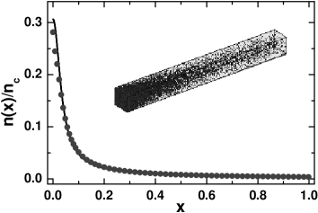
Figure 1: The rescaled density profiles obtained from the hydrostatic equations (line) and from MD simulations (circles). The dimensionless parameters are $\Lambda=5\times 10^{3}$ and $f=0.02317$, the MD simulation parameters are $L_{x}=500d$, $L_{y}=L_{z}=50d$, $N=40960$ and $r=0.9904$. The inset shows a typical snapshot of the system at the steady state as observed in the MD simulation.

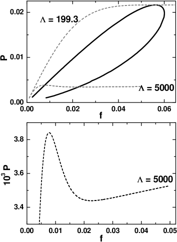
Figure 2: Upper panel: the rescaled steady state granular pressure $P$ versus the grain volume fraction $f$ for $\Lambda=199.3$ and $\Lambda=5\times 10^{3}$. Shown by the solid line is the spinodal balloon, inside which the effective lateral compressibility of the gas is negative. The borders $f_{1}$ and $f_{2}$ of the spinodal interval are determined from the condition $\left(\partial P/\partial f\right)_{\Lambda}=0$. Lower panel: a zoom-in at the $P(f)$ dependence for $\Lambda=5\times 10^{3}$.

Having found the density profiles at different $\Lambda$ and $f$, we can compute, with the help of Eq. (2), the rescaled pressure of the layer state $P=p/(n_{c}T_{0})$. As the steady-state pressure is constant throughout the system, one can compute it at the thermal wall $x=1$, where the temperature $T=T_{0}$ is prescribed knudsen . We obtain, therefore,

$$P(f,\Lambda)=\frac{1+4G[U(1)]}{U(1)}\,.$$

Two typical $P(f)$ curves for different $\Lambda$ are shown in Fig. 2. At small $\Lambda$ (exemplified by $\Lambda=199.3$) the bulk energy loss is not very important, and $P(f)$ is monotone increasing with $f$. At sufficiently large $\Lambda$ (exemplified by $\Lambda=5\times 10^{3}$) there is an interval of the volume fractions $f_{1}(\Lambda)<f<f_{2}(\Lambda)$ where the rescaled pressure $P(f)$ decreases with an increase of $f$. Therefore, the effective compressibility of the gas in the lateral directions is negative there. The lower panel of Fig. 2 shows a blowup of the negative compressibility region at $\Lambda=5\times 10^{3}$. The borders of the negative compressibility region are determined by the condition $\left(\partial P/\partial f\right)_{\Lambda}=0$. By joining the spinodal points $f_{1}$ and (separately) $f_{2}$ at different $\Lambda$, we obtain the spinodal balloon of the system in the $(P,f)$ plane (Fig. 2), or in the $(\Lambda,f)$ plane (Fig. 3). As $\Lambda$ decreases, the spinodal interval $f_{1}(\Lambda)<f<f_{2}(\Lambda)$ shrinks into a point, as in the 2D case argentina ; khain2 . This is the critical point of the system $(P_{c},f_{c})$, or $(\Lambda_{c},f_{c})$. At $\Lambda<\Lambda_{c}$ $P(f)$ is monotone increasing.

A negative lateral compressibility implies that, within the spinodal balloon, the layer state [a 1D solution of the steady state equation (5)] is unstable with respect to small-amplitude long-wavelength perturbations in one or both lateral directions. Similarly to the well-studied 2D setting argentina ; khain2 there is also a binodal (or coexistence) line, originating from the intervals of area fractions where the layer state, although linearly stable, is nonlinearly unstable (that is, metastable). The two branches of the binodal line in the $(\Lambda,f)$ plane merge at the same critical point $(\Lambda_{c},f_{c})$. The asymptote of the binodal line in a close vicinity of the critical point, $|f-f_{c}|\ll f_{c}$ and $0<\Lambda-\Lambda_{c}\ll\Lambda_{c}$, can be readily established, cf. Refs. argentina ; khain2 . Indeed, in the close vicinity of the critical point $P(f)$ is describable, at fixed $\Lambda$, by a cubic parabola in $f-f_{c}$ without a quadratic term. As a result, one can find, at fixed $\Lambda$, the two points $f_{-}$ and $f_{+}$, belonging to the binodal line, from the simple relations $P(f_{-},\Lambda)=P(f_{+},\Lambda)$ and $f_{-}+f_{+}=2f_{c}$. The resulting binodal asymptote is depicted in Fig. 3.

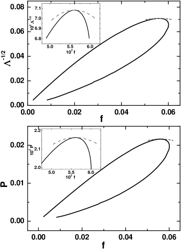
Figure 3: The spinodal balloon of the system (the solid line) and the asymptote of the binodal line in a close vicinity of the critical point (the dashed line) on the plane $f,\Lambda^{-1/2}$ (the upper panel) and on the plane $f,P$ (the lower panel). The insets zoom in on a close vicinity of the critical point.

Unfortunately, this simple asymptote cannot be continued beyond the close vicinity of the critical point. The form of the binodal line far from the critical point has not yet been derived from granular hydrodynamics, neither in 2D, nor in 3D. Such a derivation would require a non-perturbative solution of the nonlinear PDE (5). Most likely, this can only be done numerically. Note that the “Maxwell construction”, suggested in Ref. argentina for the binodal line in 2D, is valid only in a close vicinity of the critical point, where it is reducible to the two simple relations $P(f_{-},\Lambda)=P(f_{+},\Lambda)$ and $f_{-}+f_{+}=2f_{c}$. The reader is advised to consult with Ref. khain2 for a more detailed discussion of this issue.

II.3 The critical value of lateral dimensions: a marginal stability analysis

When the dimensionless parameters $\Lambda$ and $f$ are within either spinodal, or binodal balloon, a steady state with a broken lateral symmetry should develop. However, the phase separation demands a sufficiently large lateral size of the system. It will be suppressed by the lateral heat conduction if the lateral aspect ratios $\Delta_{y}$ and $\Delta_{z}$ are both less than a critical value $\Delta_{c}(\Lambda,f)$. By analogy with 2D, see Refs. livne1 ; khain1 ; livne2 ; baruch2 , we can determine $\Delta_{c}(\Lambda,f)$ from a marginal stability analysis. Indeed, let $\Delta_{y}$ and $\Delta_{z}$ be less than $\Delta_{c}(\Lambda,f)$, so the layer state is linearly stable, because of the lateral heat conduction, even within the spinodal balloon. Increasing $\Delta_{y}$ and/or $\Delta_{z}$ slightly beyond $\Delta_{c}(\Lambda,f)$, one should observe a (weakly) phase separated steady state that bifurcates supercritically from the layer state. Therefore, close to the bifurcation point, this weakly phase separated steady state can be found by linearizing Eq. (5) around the layer state $u=U(x)$. In the time-dependent hydrodynamic framework, this linear analysis corresponds to a marginal stability analysis of the layer state with respect to small perturbations in the $y$- and $z$-directions.

Substituting $u(x,y,z)=U(x)+\psi_{k}(x)\cos k_{y}y\,\cos k_{z}z$ into Eq. (5) and linearizing with respect to the small correction $\psi_{k}(x)\cos k_{y}y\cos k_{z}z$, we obtain the following linear equation for the new function $\phi_{k}(x)\equiv F\,\psi_{k}(x)$:

$$\phi_{k}^{\prime\prime}(x)-\left(k^{2}+\frac{\Lambda Q_{U}}{F}\right)\phi_{k}(x)=0\,.$$ (9)

Here $k^{2}=k_{y}^{2}+k_{z}^{2}$, the functions $F$ and $Q$ are evaluated at $u=U(x)$, and $Q_{U}$ denotes the $u$ derivative of $Q(u)$ evaluated at $u=U(x)$. The boundary conditions for Eq. (9) are

$$\phi_{k}^{\prime}(x=0)=0\,\;\;\;\;\mbox{and}\;\;\;\;\;\;\phi_{k}(x=1)=0\,.$$ (10)

Equation (9) can be interpreted as a Schrödinger equation for a single particle in a one-dimensional potential $V(x)=\Lambda Q_{U}/F$, while the quantity $-k^{2}$ serves as the (negative or zero) energy eigenvalue. We solved this eigenvalue problem numerically for different $\Lambda$ and $f$. Figure 4 shows the resulting marginal stability curves $k_{*}=k_{*}(f)$ for four different values of $\Lambda>\Lambda_{c}$. Assuming that the instability is non-oscillatory at the onset, one can interpret the marginal stability results as linear instability of the layer state below the corresponding curve, and linear stability above the curve. The instability is possible only within the spinodal balloon: the borders $f_{1}$ and $f_{2}$ of the spinodal interval correspond, at fixed $\Lambda$, to zero eigenvalues $k\to 0$.

Figure 4: Marginal stability curves for four different values of $\Lambda$ are plotted in rescaled coordinates: $k\Lambda^{-1/2}$ versus $f\Lambda^{1/2}$. For a fixed $\Lambda$ the layer state is linearly stable above the corresponding curve and unstable below the curve.

It can be seen in Fig. 4 that, in the rescaled coordinates, the marginal stability curves for different $\Lambda$ originate (almost) at the same point of the horizontal axis $f\Lambda^{1/2}$. Furthermore, the maxima of all the curves are almost equal. Like in the 2D case, the first property can be explained analytically by considering the dilute limit of the problem, while the second property results from the strong localization of the eigenfunctions $\phi_{k}(x)$ near the elastic wall khain1 .

Having found the eigenvalues $k_{*}(f,\Lambda)$, we can determine the critical (minimum) lateral aspect ratios for a phase separation. Indeed, the zero heat flux conditions at the walls $y=0,\,y=\Delta_{y},\,z=0$ and $z=\Delta_{z}$ (recall that we are using rescaled coordinates) yield the quantization rules $k_{y}=(n_{y}\pi)/\Delta_{y}$ and $k_{z}=(n_{z}\pi)/\Delta_{z}$, where $n_{y},n_{z}=0,1,2,\dots$. Therefore, the minimum value of $\Delta_{y}$ ($\Delta_{z}$) for a phase separation only in the $y$-direction (correspondingly, only in the $z$-direction) is $\Delta_{y}^{c}=\Delta_{z}^{c}=\pi/k_{*}(f,\Lambda)$. For example, for $\Lambda=8\times 10^{3}$ and $f=0.011$ we obtain $k^{2}_{*}\simeq 21.0$, therefore $\Delta_{y}^{c}=\Delta_{z}^{c}=\pi/k_{*}\simeq 0.69$. In order to have a phase separation in both lateral directions $y$ and $z$, the aspect ratios $\Delta_{y}$ and $\Delta_{z}$ must obey the inequality

$$\frac{1}{\Delta_{y}^{2}}+\frac{1}{\Delta_{z}^{2}}<\frac{k_{*}^{2}(f,\Lambda)}{\pi^{2}}\,.$$

III MD Simulations

III.1 Method

We performed a series of event-driven MD simulations of this 3D system using a standard algorithm described by Rapaport rapaport . Simulations involved $N$ hard spheres of diameter $d=1$ and mass $m=1$. After each collision of particle $i$ with particle $j$, their relative velocity was updated according to

$$\vec{v}_{ij}^{\,\prime}=\vec{v}_{ij}-\left(1+r\right)\left(\vec{v}_{ij}\cdot\hat{r}_{ij}\right)\hat{r}_{ij}\,,$$ (11)

where $\vec{v}_{ij}$ is the precollisional relative velocity, and $\hat{r}_{ij}\equiv\vec{r}_{ij}/\left|\vec{r}_{ij}\right|$ is a unit vector connecting the centers of the two particles. The “thermal” wall was kept at constant temperature $T_{0}$ that we set to unity. We used a standard thermal wall implementation, see e.g. Ref. thorsten3 , p. 173-177. Particle collisions with the rest of the walls were assumed elastic. The natural time unit of the MD simulations is $d(m/T_{0})^{1/2}=1$. The initial spatial distribution of (non-overlapping) particles was uniform in all simulations. The initial particle velocity distribution was uniform in the direction angles, while the absolute value $v_{0}$ of the velocity of each particle was chosen to be such that $(1/2)\,mv_{0}^{2}=(3/2)(1-1/N)T_{0}$. In all simulations the velocity of the center of mass of the particles at $t=0$ was zero. That the transients died out and the system reached a steady state was monitored by (i) measuring the total energy of all particles versus time, and (ii) measuring the coordinates of the center of mass versus time.

As a test simulation, we performed a simulation of a system which dimensionless parameters $\Lambda$ and $f$ are within the spinodal balloon but which still cannot phase separate because of too small lateral dimensions, see Fig. 1. The inset shows a late-time snapshot of the system as observed in the MD simulation. As one can see from Fig. 1, the measured particle number density, rescaled to $n_{c}$, as a function of the rescaled distance from the driving wall is in good agreement with our hydrostatic calculations.

III.2 Phase separation

Remaining within the spinodal balloon, and increasing one of the lateral dimensions of the system, we observed phase separation as expected from the theory, see Fig. 5. A dense cluster develops in one of the two corners of this quasi-2D Hele-Shaw cell, at the wall opposite to the driving wall. Quantitative diagnostics are provided by the plots of the three center-of-mass coordinates of the system versus time, shown in the lower panel of Fig. 5.

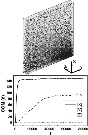
Figure 5: Upper panel: a late-time snapshot of an MD simulation with $N=10^{5}$ particles of $r=0.89945$ in the container with dimensions $L_{x}=L_{y}=500d$ and $L_{z}=50d$. The upper wall is the driving wall. The dimensionless parameters of the system $\Lambda=5\times 10^{4}$ and $f=0.0057$ correspond to a point within the spinodal balloon of Fig. 2. Lower panel: the absolute values of the three center-of-mass (COM) coordinates (measured in the units of the particle diameter $d$) versus time [measured in the units of $d(m/T_{0})^{1/2}$]. The center of the container is at the origin.

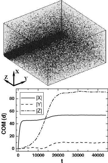
Figure 6: Upper panel: a late-time snapshot of an MD simulation with $N=5\times 10^{5}$ particles of $r=0.899452$ in the container with dimensions $L_{x}=200d$ and $L_{y}=L_{z}=400d$. The upper wall is the driving wall. The dimensionless parameters of the system $\Lambda=8\times 10^{3}$ and $f=0.011$ correspond to a point within the spinodal balloon of Fig. 2. Lower panel: same as in Fig. 5.

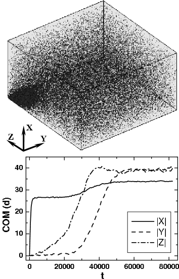
Figure 7: Upper panel: a late-time snapshot of an MD simulation with $N=340736$ particles of $r=0.899452$ in the container with dimensions $L_{x}=200d$ and $L_{y}=L_{z}=400d$. The upper wall is the driving wall. The dimensionless parameters of the system $\Lambda=8\times 10^{3}$ and $f=7.529\times 10^{-3}$ correspond to a point within the spinodal balloon of Fig. 2. Lower panel: same as in Fig. 5.

Figure 6 shows another example of phase separation for $\Lambda$ and $f$ within the spinodal balloon, but this time in the case when both lateral dimensions $L_{y}$ and $L_{z}$ are sufficiently large. As one can see, a dense stripe-like cluster forms along one of the edges of the wall opposite to the driving wall.

Both Fig. 5, and Fig. 6 show phase separated states with a 2D, rather than 3D, structure. An example of a fully 3D structure is shown in Fig. 7. Here a fully 3D dense cluster (a “drop”) develops in one of the corners at the wall opposite to the driving wall.

IV Discussion

As we have shown, granular hydrodynamics predicts negative lateral compressibility and, therefore, phase-separation instability of the basic state of a granulate driven by a thermal wall of a rectangular container at zero gravity. When the lateral dimensions of the container are sufficiently large, the negative compressibility causes a van der Waals-like phase separation instability.

Our MD simulations are in agreement with hydrostatic predictions (of course, if we disregard small fluctuations caused by the discreteness of the particles). In the language of hydrostatics, a broken-symmetry steady state is described by either a 2D, or a fully 3D solution of the nonlinear partial differential equation (5) subject to the fixed mass constraint (7) and the boundary conditions. Such steady-state solutions can be obtained only numerically (see Ref. livne1 for 2D examples). Because of the translational symmetry of the steady-state equations in the $y$ and $z$ directions, bounded solutions satisfying the no-flux boundary conditions in these directions, must be either independent of the $y$ and $z$ coordinates, or periodic in them. Furthermore, by analogy with the 2D setting, one should expect that dynamic coarsening selects a periodic steady state solution with a maximum spatial period (equal to twice the container size in the corresponding direction livne2 ).

When one of the lateral aspect ratios, say $\Delta_{y}$, is larger than the critical value $\Delta_{c}(\Lambda,f)$, while the other one, $\Delta_{z}$, is smaller than $\Delta_{c}$, a 2D pattern should develop, and this is indeed what we observed in Fig. 5. When both of the lateral dimensions are larger than $\Delta_{c}$, we observed dense clusters of two different morphologies: either a 2D morphology, like the one shown in Fig. 6, or a fully 3D morphology, like the one shown in Fig. 7.

What will happen when the parameters $\Lambda$ and $f$ are within the spinodal or binodal balloons, and its lateral dimensions $L_{x}$ and $L_{y}$ are much larger than $\Delta_{C}$? We expect that multiple “drops” (or bubbles) will nucleate at the wall opposite to the driving wall and undergo dynamic coarsening, qualitatively similar to Ostwald ripening Ostwald , before reaching the final state with a single drop (or bubble). The Ostwald ripening regime is beyond the reach of our present computing resources.

When the lateral aspect ratios $\Delta_{y}$ and $\Delta_{z}$ are just above (or just below) the critical value $\Delta_{c}=\Delta_{c}(\Lambda,f)$, the phase separation, as predicted by hydrostatics, should be “weak” and look, in the supercritical case, as a small-amplitude modulation of the layer state livne1 ; brey2 ; khain1 ; livne2 ; baruch2 ; khain2 . In 2D such a system experiences large fluctuations baruch2 , and it would be interesting to find out whether large fluctuations persist in 3D.

We also performed a series of MD simulations for more realistic conditions, using a (truly) vibrating wall instead of the thermal wall, and allowing for inelastic particle collisions with the walls. Qualitatively, the results have not changed: for sufficiently high inelasticity of particle-particle collisions we observed phase separation for intermediate values of the volume fraction, and no phase separation for too a small or too a large volume fraction.

Our theory and simulations assumed a a zero gravity. To what extent is the van der Waals-like phase transition sensitive to the presence of a small gravity, with acceleration $g$, directed towards the thermal wall? In a 2D setting this question was addressed by Khain and Meerson khainconv . Assuming dilute limit of granular hydrodynamics, they found that, as the Froude number $F=mgL_{x}/T_{0}$ increases, the phase separation crosses over to “thermal” granular convection. One can expect a similar scenario in 3D as well, though this question has not been yet been considered in detail.

In summary, the van der Waals-like phase separation in 2D and 3D provides a useful and rich prototypical model system for testing the ideas and methods of granular dynamics. By focusing our attention on 3D in this work, we broke ground for a future investigation of this fascinating phase separation phenomenon in reduced gravity experiments.

- (1) G. H. Ristow, Pattern Formation in Granular Materials (Springer Tracts in Modern Physics) (Springer, Berlin, 2000).
- (2) I. S. Aranson and L. S. Tsimring, Rev. Mod. Phys. 78, 641 (2006).
- (3) C. S. Campbell, Annu. Rev. Fluid Mech. 22, 57 (1990).
- (4) L. P. Kadanoff, Rev. Mod. Phys. 71, 435 (1999).
- (5) Granular Gases, edited by T. Pöschel and S. Luding (Springer, Berlin, 2001).
- (6) Granular Gas Dynamics, edited by T. Pöschel and N. Brilliantov (Springer, Berlin, 2003).
- (7) I. Goldhirsch, Annu. Rev. Fluid Mech. 35, 267 (2003).
- (8) N. V. Brilliantov and T. Pöschel, Kinetic Theory of Granular Gases (Oxford University Press, Oxford, 2004).
- (9) E. Livne, B. Meerson, and P. V. Sasorov, Phys. Rev. E 65, 021302 (2002); cond-mat/0008301 (2000).
- (10) M. Argentina, M. G. Clerc, and R. Soto, Phys. Rev. Lett. 89, 044301 (2002); M.G. Soto, M. Argentina, and M.G. Clerc, in Ref. thorsten2 , p. 317.
- (11) J. J. Brey, M. J. Ruiz-Montero, F. Moreno, and R. García-Rojo, Phys. Rev. E 65, 061302 (2002).
- (12) E. Khain and B. Meerson, Phys. Rev. E 66, 021306 (2002).
- (13) E. Livne, B. Meerson, and P. V. Sasorov, Phys. Rev. E 66, 050301(R) (2002).
- (14) B. Meerson, T. Pöschel, P. V. Sasorov, and T. Schwager, Phys. Rev. E 69, 021302 (2004).
- (15) E. Khain, B. Meerson, and P. V. Sasorov, Phys. Rev. E 70, 051310 (2004).
- (16) C. Cartes, M. G. Clerc, and R. Soto, Phys. Rev. E 70, 031302 (2004).
- (17) A. Kudrolli, M. Wolpert, and J. P. Gollub, Phys. Rev. Lett. 78, 1383 (1997).
- (18) E. L. Grossman, T. Zhou, and E. Ben-Naim, Phys. Rev. E 55, 4200 (1997).
- (19) M. Díez-Minguito and B. Meerson, Phys. Rev. E 75, 011304 (2007).
- (20) In the Knudsen layer at the thermal wall the gas temperature is actually smaller than the wall temperature. This is the well-known Knudsen effect that also occurs in ordinary gases chapman . The Knudsen effect is small once the size of the Knudsen layer (which is of the order of the mean free path of the gas near the thermal wall) is much less than the characteristic length scale of the hydrostatic profile. Our hydrostatic model neglects the Knudsen effect.
- (21) N. F. Carnahan and K. E. Starling, J. Chem. Phys. 51, 635 (1969).
- (22) J. T. Jenkins and M. W. Richman, Arch. Rat. Mech. Anal. 87, 355 (1985).
- (23) H. B. Keller and D. S. Cohen, J. Math. Mech. 16, 1361 (1967).
- (24) D. C. Rapaport, The Art of Molecular Dynamics Simulation (Cambridge University Press, Cambridge, 1997).
- (25) T. Pöschel and T. Schwager, Computational Granular Dynamics: Models and Algorithms (Springer, Berlin, 2005).
- (26) W. Ostwald, Z. Phys. Chem., Stoechiom. Verwandtschaftsl 34, 495 (1900).
- (27) E. Khain and B. Meerson, Phys. Rev. E 67, 021306 (2003).
- (28) S. Chapman and T.G. Cowling, The Mathematical Theory of Non-Uniform Gases (Cambridge Univ. Press, Cambridge, 1990), p. 101.