Deriving temperature, mass and age of evolved stars from high-resolution spectra

Abstract

Aims. We test our capability of deriving stellar physical parameters of giant stars by analysing a sample of field stars and the well studied open cluster IC 4651 with different spectroscopic methods.

Methods. The use of a technique based on line-depth ratios (LDRs) allows us to determine with high precision the effective temperature of the stars and to compare the results with those obtained with a classical LTE abundance analysis.

Results. ($i$) For the field stars we find that the temperatures derived by means of the LDR method are in excellent agreement with those found by the spectral synthesis. This result is extremely encouraging because it shows that spectra can be used to firmly derive population characteristics (e.g., mass and age) of the observed stars. ($ii$) For the IC 4651 stars we use the determined effective temperature to derive the following results. a) The reddening $E(B-V)$ of the cluster is $0.12\pm 0.02$, largely independent of the color-temperature calibration used. b) The age of the cluster is $1.2\pm 0.2$ Gyr. c) The typical mass of the analysed giant stars is $2.0\pm 0.2M_{\sun}$. Moreover, we find a systematic difference of about 0.2 dex in $\log g$ between spectroscopic and evolutionary values.

Conclusions. We conclude that, in spite of known limitations, a classical spectroscopic analysis of giant stars may indeed result in very reliable stellar parameters. We caution that the quality of the agreement, on the other hand, depends on the details of the adopted spectroscopic analysis.

1 Introduction

The detailed study of stellar populations in our own Galaxy and in its neighborhoods has received a major impulse in the last years, thanks to the use of large telescopes coupled to multi-object high-resolution spectrographs.

The spectroscopic determination of chemical abundances in the atmospheres of stars may greatly contribute to our knowledge of galaxies. In fact, once a set of chemical abundances is complemented with a stellar age, it is possible to assess the age-metallicity relation, and to invert the observed color-magnitude diagram (CMD) thus obtaining the Star Formation History (SFH) of the Galaxy (see, e.g., Tolstoy 2005, and the Large Magellanic Cloud case illustrated by Cole et al. 2005). When individual stellar ages are unknown, this analysis becomes more uncertain because of the so-called age-metallicity degeneracy, i.e. the fact that old metal-poor stars can occupy the same region of the CMD as young metal-rich objects.

In this context, open clusters provide fundamental tools because each cluster represents an homogeneous sample of stars having the same age and chemical composition. Moreover, they are very suitable for the investigation of several issues related to stellar and Galactic formation and evolution. In particular, young open clusters provide information about present-day star formation processes and are key objects for clarifying questions on galactic structure, while old and intermediate-age open clusters play an important role in linking the theories of stellar and galactic evolution.

The main classical tool to study cluster properties is the color-magnitude diagram, which suffers from several uncertainties and intrinsic biases, such as the limited knowledge of the chemical composition of the stars and the degeneracy in deriving the distance (and therefore age) and reddening. As a consequence, the photometric analysis of open clusters alone might not be so conclusive for an accurate determination of ages, distances, metallicities, masses, color excesses, and temperatures, as shown by Randich et al. (2005). Thus, spectroscopic methods to determine the effective temperature of cluster members are efficient techniques that are independent of the cluster reddening. This reddening can then be obtained by comparing the spectroscopic results to the photometric ones.

Effective temperatures can be determined by imposing the condition that the derived abundance for one chemical element with many lines in the spectrum (typically Fe i) does not depend on the excitation potentials of the lines (hereafter this technique will be called as “spectral synthesis” and the “spectroscopic temperature” derived in this way will be indicated $T_{\mathrm{eff}}^{\rm SPEC}$). Another spectroscopic method is based on the ratio of the depths of two lines having different sensitivity to effective temperature. This line-depth ratios (LDRs) technique provides an excellent measure of stellar temperature (hereafter $T_{\mathrm{eff}}^{\rm LDR}$) with a sensitivity as small as a few Kelvin degrees in the most favorable cases (Gray & Johanson 1991; Strassmeier & Schordan 2000; Gray & Brown 2001).

In this paper we apply the LDR method to derive effective temperature of nearby evolved field stars with good Hipparcos parallaxes (accuracy better than 10%, da Silva et al. 2006) and of giant stars of the intermediate-age open cluster IC 4651. For both groups, the temperature was previously derived photometrically by means of color indices and spectroscopically by abundance studies (Pasquini et al. 2004; da Silva et al. 2006). In this work, we compare $T_{\mathrm{eff}}^{\rm LDR}$ with the previous photometric and spectroscopic determinations in order to check temperatures obtained with different methods, and to understand the temperature range in which each method can be used. This will verify how accurately physical parameters can be obtained by inverting the spectroscopic results. Moreover, for the stars belonging to the open cluster IC 4651, we are able to derive in a “spectroscopic way” color excess, mass and age. This is an important test because, to our knowledge, this is the first time that these parameters are determined in a cluster by means of the line-depth ratio method. Moreover, the possibility of comparing our spectroscopic results on IC 4651 with those obtained by the classical fitting of the main sequence provides a unique opportunity to cross-check our inversion method.

2 Sample selections and observations

We have considered seventy-one evolved field stars and six giant stars belonging to the intermediate-age open cluster IC 4651.

The sample of field stars has been selected and analysed by Setiawan et al. (2004) to derive the radial velocity (RV) variations along the Red Giant Branch and to investigate the nature of the radial velocity long-term variations. Subsequently, the same sample was studied by da Silva et al. (2006) for the determination of radii, temperatures, masses, and chemical composition with the aim to understand how the RV variability is related to the stellar physical parameters.

The stars in the cluster IC 4651 have been taken from the sample of Pasquini et al. (2004). The evolutionary status of the analysed stars is indicated by their position in the CMD shown in Fig. 1 in which our stellar sample is marked with arrows.

The details of the observations, data reduction, and instrumentation are described in Setiawan et al. (2004) and Pasquini et al. (2004). Their main characteristics are briefly summarized here. The spectra of the field stars were acquired with the FEROS spectrograph ($R=48\,000$, Kaufer et al. 1999) at the ESO 1.5m-telescope in La Silla (Chile), while the IC 4651 spectra were acquired with the UVES spectrograph ($R=100\,000$, Dekker et al. 2000) at the ESO VLT Kueyen 8.2m-telescope in Cerro Paranal (Chile). The FEROS spectrograph has a wavelength coverage between 3700 and 9200 Å, while the spectral region of the UVES observations covers the 5800$-$6800 Å range (we have selected the data acquired by Pasquini et al. 2004 with the CD#3 since they covered the spectral region of our interest). The signal-to-noise ($S/N$) ratio in all cases is higher than 150/pixel and 160/pixel for the FEROS and UVES spectra, respectively.

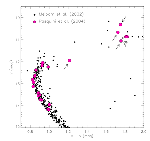
Figure 1: CMD of IC 4651. $V$ and $v-y$ are taken from Anthony-Twarog et al. (1988) and Meibom et al. (2002), respectively. The stars analysed by Meibom et al. (2002) and Pasquini et al. (2004) are indicated by different symbols, while our ones are marked with arrows.

3 Data analysis

3.1 Effective temperature

The spectral regions covered by FEROS and UVES contain a series of weak metal lines which can be used for temperature determination with the LDR method. Lines from similar elements such as iron, vanadium, titanium, but with different excitation potentials ($\chi$) have different sensitivity to temperature. This is because the line strength is a function of temperature and, to a lesser extent, of the electron pressure (and consequently, the surface gravity). This sensitivity arises from the exponential and power dependence on temperature in the excitation and ionization processes. Different lines are formed at different depths of the stellar atmosphere and therefore one would expect that lines from levels with high excitation potentials are formed deeper in the atmosphere and hence at higher temperatures. For this reason, it is better to choose pairs of lines with the largest $\chi$-difference. Between 6180 Å and 6280 Å there are several lines of this type whose depth ratios have been exploited for temperature calibrations (Gray & Johanson 1991; Gray & Brown 2001; Catalano et al. 2002; Biazzo et al. 2007a), to study the rotational modulation of the average effective temperature of magnetically active stars (Frasca et al. 2005; Biazzo et al. 2007b) or to investigate in Cepheid stars the pulsational variations with phases (Kovtyukh & Gorlova 2000; Biazzo et al. 2004). In particular, we chose 15 weak line pairs for which Biazzo et al. (2007a) made suitable calibrations. These lines are of elements belonging to the iron group that have different temperature sensitivity. Furthermore, the $S/N$ ratio around 150 for all the spectra makes them very suitable for the LDR method, because with such a high $S/N$ ratio a precision of a few Kelvin degree is expected (Gray & Johanson 1991; Gray & Brown 2001; Kovtyukh et al. 2006; Biazzo et al. 2007a).

3.1.1 Sample of field stars

All the field stars analysed in this paper have low rotational velocity ($v\sin i<7$ km s^-1). The spectral resolution of FEROS is quite similar to that of the spectrograph ELODIE (Observatoire de Haute-Provence, France), used by Biazzo et al. (2007a). As a consequence, the LDR$-T_{\mathrm{eff}}$ calibrations developed by Biazzo et al. (2007a) at $v\sin i\leq 5$ km s^-1 have been applied to derive the effective temperature ($T_{\mathrm{eff}}^{\rm LDR}$). Our star sample is comprised of sixty-seven giants and four stars with log $g>$ 4.0 (namely HD2151, HD16417, HD26923 and HD62644), as derived by da Silva et al. (2006). For the latter the LDR$-T_{\mathrm{eff}}$ calibration for main sequence stars obtained by Biazzo et al. (2007a) has been used.

We would like to note that Biazzo et al. (2007a) adopted the color-temperature relationship obtained by Gray (2005), which does not include corrections due to metallicity. We shall come back to this point in the discussion of the Sections 4.1.1 and 4.2.1.

3.1.2 IC 4651

For the giant stars of IC 4651, the UVES spectra have $R=100\,000$, significantly higher than the ELODIE ($R=42\,000$), so, in order to apply the calibrations, it was necessary to degrade the UVES spectra to the resolution of ELODIE. The analysed six giant stars have rotational velocities $v\sin i$ in the range 0–15 km s^-1, thus the LDR$-T_{\mathrm{eff}}$ calibrations developed by Biazzo et al. (2007a) for the appropriate $v\sin i$ have been applied to derive the effective temperatures ($T_{\mathrm{eff}}^{\rm LDR}$). For the subgiant E95, an interpolation between the main sequence and the giant calibrations was applied. Consequently, the effective temperature uncertainty for this star should be higher than for the giants.

3.2 Surface gravity

We can compute the “photometric” surface gravity using the relation $\log g=\log g_{\sun}+\log(M/M_{\sun})+4\log(T_{\mathrm{eff}}/T_{\rm eff,\sun})-\log(L/L_{\sun})$, where $g_{\sun}$ is the solar surface gravity, while $M$, $T_{\mathrm{eff}}$ and $L$ are the stellar mass, photometric effective temperature, and luminosity in the respective solar units.

3.3 Reddening

Several determinations of the photometric reddening of IC 4651 exist in literature (see, e.g., Meibom et al. 2002, and reference therein). Once the spectroscopic temperatures have been derived, we can estimate for each star the intrinsic color index ($B-V$)₀ by inverting the $(B-V)_{0}-T_{\mathrm{eff}}$ relation and to compute the color excess $E(B-V)$ from the observed and reddened $(B-V)$ color. This can be obtained for each star separately, therefore the statistics on all stars can tell us not only the reddening of the cluster, but also provide a check of the goodness of the method applied.

3.4 Mass and Age

Mass and age are estimated using a slightly modified version of the Bayesian estimation method conceived by Jørgensen & Lindegren (2005), as da Silva et al. (2006) proposed (see references therein for more information). In short, given the stellar absolute magnitude, effective temperature, metallicity, and the associate errors, we can estimate the probability that such a star belongs to each small section of a theoretical stellar isochrone of a given age and metallicity. In particular, we have considered the isochrones developed by Girardi et al. (2000). Then, the probabilities are summed over the complete isochrone, and hence over all possible isochrones, by assuming a Gaussian probability of having the observed metallicity and its error, and a constant probability of having stars of all ages. The latter assumption is equivalent to assuming a constant star formation rate in the solar neighbourhood. In this way, at the end, we have the age probability distribution function (PDF) of each observed star. PDFs can also be obtained for any stellar property, such as initial mass, surface gravity, intrinsic colour, etc.

Although a full discussion of the PDF method is beyond the scope of this paper, we note the following. The method, with just some small differences, has already been tested on both main sequence stars (Nordström et al. 2004) and on giants and subgiants (da Silva et al. 2006). Ages of dwarfs turn out to be largely undetermined by this method, due to their very slow evolution while on the main sequence. Ages of giants turn out to be well determined provided that the effective temperature and the parallax (absolute magnitude) are measured with enough accuracy. In fact, da Silva et al. (2006) find that stars with errors of 70 K in $T_{\rm eff}$, and less than 10% errors in parallaxes, have ages determined with an accuracy of about 20%. These errors become larger for particular regions of the CMD, for instance on the red clump region, where stars of very different age and metallicity become tightly clumped together, and where in addition there is a superposition of red clump stars and first-ascent RGB ones. On the other hand, the best age determinations are expected on the subgiant branch region of the CMD, where evolutionary tracks of different masses separate very well from each other. To some extent, also the lower part of the red giant branch provides good age determinations, since in this CMD region there is no superposition with other evolutionary stages and stars above a given absolute magnitude can only be fitted by stars below a given mass (and above a given age).

Of course, the above-mentioned errors do not include the systematic errors that may hide in the stellar evolutionary tracks and isochrones used. In fact, in any set of evolutionary tracks the position of the giants depends on the choice of mixing length parameter (usually calibrated on the Sun), and to a much smaller extent on details of solving the atmosphere structure and on the interpolation of opacity tables. The only way to avoid this kind of uncertainty would be the building of tracks (and isochrones) in which the theory of energy transport and atmospheric structure are accurately calibrated on observations of star clusters and binaries. This approach however is still too far to reach. Using the PDF method with different sources of evolutionary tracks could provide hints on the magnitude of systematic errors, but would not solve the situation because different sets of tracks in the literature do share the same assumptions and input physics.

Therefore, at present we cannot reliably evaluate the systematic errors present in the PDF method. A simple check with two Hyades giants, where the PDF ages can be compared with the turn-off ones, hints to an accuracy of about 20% for the objects studied by da Silva et al. (2006). It would be extremely interesting to perform similar tests using giants in clusters of a wide range of ages, although we know that their distances (and turn-off ages) would be significantly more uncertain than the Hyades ones.

4 Results

4.1 Sample of field stars

4.1.1 Effective temperature

In Table 1 we list names, $T_{\mathrm{eff}}^{\rm LDR}$ together with the photometric ($T_{\mathrm{eff}}^{\rm PHOT}$) and spectroscopic ($T_{\mathrm{eff}}^{\rm SPEC}$) temperatures, and as well as the stellar abundances retrieved by da Silva et al. (2006). The photometric temperatures were determined using the $(B-V)-T_{\mathrm{eff}}$ relationships of Alonso et al. (1996, 1999) for dwarf and giant stars.

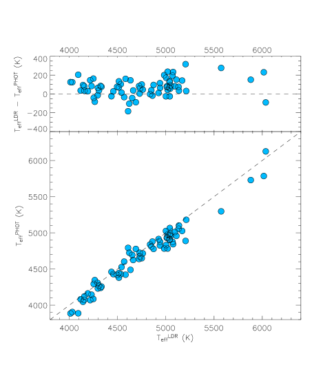
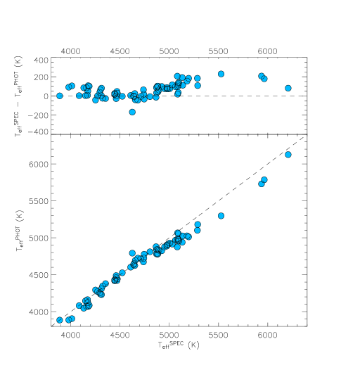
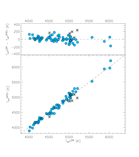
Figure 2: Comparison between effective temperatures obtained by line-depth ratio, spectral synthesis, and photometric methods. The second plot ($T_{\mathrm{eff}}^{\rm PHOT}$ vs. $T_{\mathrm{eff}}^{\rm SPEC}$) shows the results obtained by da Silva et al. (2006). The asterisks in the third plot represent the five metal-deficient ([Fe/H]$<-0.4$) stars in our sample.

The comparison between these three temperatures is emphasized in Fig. 2 and discussed here in the following.

• The temperatures derived by spectral synthesis ($T_{\mathrm{eff}}^{\rm SPEC}$) and by LDR method ($T_{\mathrm{eff}}^{\rm LDR}$) are higher than the photometric ones by about 60–70 K, on average. This indicates that the photometric techniques tend to underestimate the temperature compared to the spectroscopic ones. This result seems to be more evident for the hottest stars in our sample.

• The agreement between $T_{\mathrm{eff}}^{\rm PHOT}$ and the $T_{\mathrm{eff}}^{\rm SPEC}$ is better in the temperature range 4000–5300 K, as already found by da Silva et al. (2006) and displayed in the top-right panel of Fig. 2. The good agreement between $T_{\mathrm{eff}}^{\rm PHOT}$ and $T_{\mathrm{eff}}^{\rm SPEC}$ or $T_{\mathrm{eff}}^{\rm LDR}$ in the 4000–5300 K temperature range is likely due to the fact that all these field stars are nearby and, consequently, the reddening, which is the parameter that mainly influences the photometric effective temperature determination, is negligible. The temperatures derived by spectroscopic methods are instead reddening-free. At higher temperatures, the behaviour of $T_{\mathrm{eff}}^{\rm PHOT}$ versus $T_{\mathrm{eff}}^{\rm SPEC}$ or $T_{\mathrm{eff}}^{\rm LDR}$ reflects the shape of the photometric calibration used for the temperature determination.

• The temperatures obtained by means of the LDR method are in very good agreement in all the range with the spectroscopic values computed by da Silva et al. (2006), the average difference $<T_{\mathrm{eff}}^{\rm LDR}-T_{\mathrm{eff}}^{\rm SPEC}>$ being about 15 K with rms = 78 K. This rms can be considered as an estimate of the absolute error on the star temperature.

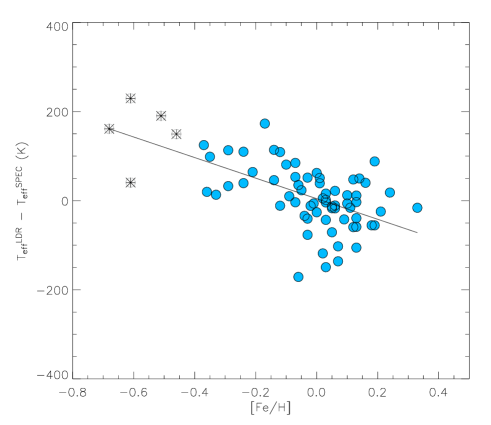
Figure 3: Metallicity dependence of $T_{\mathrm{eff}}^{\rm LDR}-T_{\mathrm{eff}}^{\rm SPEC}$. The five stars with [Fe/H]$<-$0.4 are showed with asterisks. Continuous line is the linear fit to the points.

• The $T_{\mathrm{eff}}^{\rm PHOT}$ versus $T_{\mathrm{eff}}^{\rm LDR}$ plot shows larger scatter compared to $T_{\mathrm{eff}}^{\rm PHOT}$ versus $T_{\mathrm{eff}}^{\rm SPEC}$. If we consider the whole temperature range, we obtain $<T_{\mathrm{eff}}^{\rm LDR}-T_{\mathrm{eff}}^{\rm PHOT}>=73\leavevmode\nobreak\ \mathrm{K}$ with the rms of 92 $\mathrm{K}$. The mean difference $<T_{\mathrm{eff}}^{\rm SPEC}-T_{\mathrm{eff}}^{\rm PHOT}>$ is $58\leavevmode\nobreak\ \mathrm{K}$ and the rms is 72 K. The fact that $T_{\mathrm{eff}}^{\rm PHOT}$ vs. $T_{\mathrm{eff}}^{\rm LDR}$ shows higher scatter compared to $T_{\mathrm{eff}}^{\rm PHOT}$ vs. $T_{\mathrm{eff}}^{\rm SPEC}$ can be due to the slight dependence of $T_{\mathrm{eff}}^{\rm LDR}$ on metallicity, especially for stars with [Fe/H] significantly different than zero, as pointed out by Biazzo et al. (2007a). In fact, if we plot the difference $T_{\mathrm{eff}}^{\rm LDR}-T_{\mathrm{eff}}^{\rm SPEC}$ as a function of the metallicity (Fig. 3), a residual dependence of the effective temperature on the metallicity emerges, mainly due to the metal-poor stars. If we disregard the five metal-deficient stars with [Fe/H]$<-$0.4 (asterisks in Fig. 2), the average difference $<T_{\mathrm{eff}}^{\rm LDR}-T_{\mathrm{eff}}^{\rm SPEC}>$ becomes very low (5 K) with a value of 68 K as rms. If we instead take the linear relationship (full line in Fig. 3) and correct $T_{\mathrm{eff}}^{\rm LDR}$ for the residual dependence on the metallicity, the final residuals between the two temperatures $T_{\mathrm{eff}}^{\rm LDR}$ and $T_{\mathrm{eff}}^{\rm SPEC}$ is only 48 K. The agreement is remarkably good considering that in this small scatter are included all the possible differences, such as errors in the equivalent width and in the line-depth ratio measurements, errors in the LDR–$T_{\mathrm{eff}}$ calibrations and errors in the $T_{\mathrm{eff}}$ scale of the adopted standard stars. We think that the residual dependence of $<T_{\mathrm{eff}}^{\rm LDR}-T_{\mathrm{eff}}^{\rm SPEC}>$ on the metallicity is due to the effect of [Fe/H] on LDRs that is a “second order” one compared to temperature and gravity, but can be neglected only for stars with a near solar metallicity. In order to adequately take into account this effect, a proper LDR$-T_{\mathrm{eff}}$ calibration should be done for a large sample containing many stars with well determined metallicity, spanning a wide range.

One could object that the fact the two spectroscopic temperatures ($T_{\mathrm{eff}}^{\rm LDR}$ and $T_{\mathrm{eff}}^{\rm SPEC}$) are in very good agreement should be expected, since the methods are very similar. However, there are a number of important differences that one should not, a priori, expect such a good agreement.

• The two techniques are independent. One method simply measures several LDRs and takes advantage of the LDR–temperature calibrations of standard stars. These calibrations use a $(B-V)-T_{\mathrm{eff}}$ polynomial relationship to determine the temperature of the standard stars. The other method computes the temperature from the equivalent widths eliminating any dependence of the Fe i abundance on the line excitation potential and using appropriate atmospheric models. In order to compute the Fe i abundance, the process involves the use of stellar atmospheric models, the use of line strength ($\log gf$), the determination of microturbulence ($\xi$) and gravity, a process which is not present in the LDR method. Only when all these steps are properly made, the results are similar.

• We know that the lines are formed at different stellar atmospheric levels, but if one chooses pairs of weak lines of similar elements (such as elements of the iron group), the abundance dependence is practically eliminated when the ratio between the two lines is considered. In the measure of the equivalent width, the abundance dependence is instead always present.

• The effects of macroturbulence cancel out, to the first order, when the LDR is computed because they affect all lines in the same way. These effects are not present in the equivalent width measurements.

• The continuum choice influences in a strong way the equivalent width determination. As a first approximation, this does not happen for the LDRs, because the continuum is practically the same for each line pair which are very close in wavelength.

• The rotational velocity shows its effect in the line-depth ratio computation, but can be taken into account using appropriate calibrations at proper rotational velocity (Biazzo et al. 2007a). The equivalent width measurement is not instead affected by rotational broadening (Gray 2005).

• Microturbulence is negligible when the depth ratio between a line pair is considered. The effective temperatures derived by spectral synthesis are instead obtained computing the contribution of microturbulence. As a consequence, wrong microturbulence values (also of 0.1-0.2 km s^-1) leads to wrong temperature determinations.

Given all these differences, there are no a priori reasons why the effective temperatures resulting from the spectral synthesis and LDR methods had to be similar.

Table 1: Parameters of the field stars.

Name	$T_{\mathrm{eff}}^{\rm LDR}$	$T_{\mathrm{eff}}^{\rm PHOT}$	$T_{\mathrm{eff}}^{\rm SPEC}$	[Fe/H]
	(K)	(K)	(K)
HD2114	5259	5180	5288	$-$0.03
HD2151	5973	5785	5964	$-$0.03
HD7672	5121	4957	5096	$-$0.33
HD11977	5024	4901	4975	$-$0.21
HD12438	5236	4888	4975	$-$0.61
HD16417	5872	5729	5936	0.19
HD18322	4639	4638	4637	$-$0.07
HD18885	4641	4673	4737	0.10
HD18907	5143	5056	5091	$-$0.61
HD21120	5203	5026	5180	$-$0.12
HD22663	4514	4792	4624	0.11
HD23319	4434	4526	4522	0.24
HD23940	4962	4782	4884	$-$0.35
HD26923	5985	6126	6207	$-$0.06
HD27256	5077	5012	5196	0.07
HD27371	4884	4914	5030	0.13
HD27697	4901	4876	4951	0.06
HD32887	4141	4046	4131	$-$0.09
HD34642	4775	4838	4870	$-$0.04
HD36189	5066	4875	5081	$-$0.02
HD36848	4325	4460	4460	0.21
HD47205	4604	4777	4744	0.18
HD47536	4513	4379	4352	$-$0.68
HD50778	4117	4081	4084	$-$0.29
HD61935	4820	4777	4879	$-$0.01
HD62644	5590	5297	5526	0.12
HD62902	4168	4230	4311	0.33
HD63697	4263	4346	4322	0.13
HD65695	4483	4421	4468	$-$0.14
HD70982	5035	4957	5089	$-$0.03
HD72650	4293	4307	4310	0.06
HD81797	4248	4085	4186	0.00
HD83441	4575	4624	4649	0.10
HD85035	4531	4724	4680	0.12
HD90957	4155	4121	4172	0.05
HD92588	4972	5025	5136	0.07
HD93257	4480	4602	4607	0.13
HD93773	5027	4912	4985	$-$0.07
HD99167	4030	3905	4010	$-$0.36
HD101321	4786	4810	4803	$-$0.14
HD107446	4229	4145	4148	$-$0.10
HD110014	4414	4429	4445	0.19
HD111884	4306	4270	4271	$-$0.06
HD113226	5027	4988	5086	0.09
HD115478	4252	4293	4250	0.03
HD122430	4323	4238	4300	$-$0.05
HD124882	4332	4256	4293	$-$0.24
HD125560	4395	4443	4472	0.16
HD131109	4154	4073	4158	$-$0.07
HD136014	4999	4782	4869	$-$0.46
HD148760	4564	4694	4654	0.13
HD151249	4011	3885	3886	$-$0.37
HD152334	4191	4162	4169	0.06
HD152980	4215	4069	4176	0.01
HD159194	4383	4418	4444	0.14
HD165760	4989	4929	5005	0.02
HD169370	4547	4488	4460	$-$0.17
HD174295	4979	4831	4893	$-$0.24
HD175751	4681	4715	4710	0.01
HD177389	4991	4939	5131	0.02
HD179799	4804	4879	4865	0.03
HD187195	4349	4428	4444	0.13
HD189319	4091	3887	3978	$-$0.29
HD190608	4647	4724	4741	0.05
HD198232	4902	4824	4923	0.03
HD198431	4676	4649	4641	$-$0.12
HD199665	5000	4975	5089	0.05
HD217428	5214	5101	5285	0.03
HD218527	5026	5066	5084	0.03
HD219615	5068	4842	4885	$-$0.51
HD224533	5023	4967	5062	0.00

4.2 IC 4651

4.2.1 Effective temperature

The star name and effective temperature as derived with the LDR ($T_{\mathrm{eff}}^{\rm LDR}$) and spectral synthesis ($T_{\mathrm{eff}}^{\rm SPEC}$) methods (Pasquini et al. 2004) are listed in the first three columns of Table 2. The stars with prefix “E” are from Eggen (1971), while the star with prefix “MEI” is from Meibom (2000).

$T_{\mathrm{eff}}^{\rm LDR}$ is always lower than $T_{\mathrm{eff}}^{\rm SPEC}$, by an amount between 70 and 90 K for most of the stars, a difference which is slightly larger than for the field stars. One cause is in the fact that IC 4651 is slightly metal rich ([Fe/H]$\sim$0.1, Pasquini et al. 2004). This implies that we should apply a metallicity correction of 19 K to $T_{\mathrm{eff}}^{\rm LDR}$ to all the stars (cfr. previous Section). With this correction, the offset between the two temperatures becomes of 50–70 K, with the exception of E95. In the fourth column of Table 2 the values of the effective temperature ($T_{\mathrm{eff}}^{\rm LDRc}$) derived by the LDR method and corrected for metallicity are given.

For the star E95 the difference is much larger, or 320 K. E95 is a subgiant star, as it appears from the CMD in Fig. 1. This has two major effects in the present analysis. This is the evolved star for which Pasquini et al. (2004) found the largest difference between photometric and spectroscopic temperature, and a full convergence of the solution could not be obtained. In addition, the LDR value quoted is a weighted average of the values we would obtain from the dwarfs calibration ($\sim$5700 K) and the giants calibration ($\sim$5250 K). As previously mentioned, we do expect for this star a lower accuracy in its LDR temperature determination.

The presence of only one hot subgiant in the sample does not allow us to derive firm conclusions, but it may indicate that before extending the method to stars in this portion of the HR diagram, further work is required. We note, however, that the change in temperature of 300 K for this star does not substantially change its derived age and mass, since the evolutionary tracks in this portion of the HR diagram are substantially horizontal and the evolutionary phase is extremely fast.

It is more difficult to provide a reliable estimate for the systematic effects which could be present in our results. Carretta et al. (2004), for instance, have in their sample three stars (namely 27, 76, and 146 of their paper), with magnitudes and color indices very close to those of the stars E98 and E60 of our sample. In particular, their star 146 corresponds to our E98. Yet, the spectroscopic temperatures they derive (4610, 4620 and 4720, respectively) are 180-290 K cooler than what found by Pasquini et al. (2004) for E98 and E60, and 130-240 K cooler than derived by us with the LDR method.

While a difference on a single star, of say 200 K, can be understood, a systematic effect of up to 200 K with respect to the LDR is more difficult to explain. $T_{\mathrm{eff}}^{\rm LDR}$ for these stars have been obtained on high quality spectra and by using a large number of line-depth ratios (namely 15), which makes the measurements extremely robust. As far as the calibrations are concerned, our stars occupy the linear part of the LDR$-T_{\mathrm{eff}}$ relationships, far from saturation effects. We therefore consider that the $T_{\mathrm{eff}}^{\rm LDR}$ measurement errors come mainly from the several LDR$-T_{\mathrm{eff}}^{\rm LDR}$ relationships, which give different temperature values. Any systematic shift should therefore be dominated by the adoption of different temperature scales. Since our calibrations are ultimately based on the $(B-V)-$temperature scale by Gray (2005), we verified the systematic differences in the color range of our interest ($B-V=$0.80–1.13) for a number of calibrations present in literature. In Fig. 4, we can see that for giants of $B-V\sim 0.95$ all the scales agree within 100 K, and this agreement increases ($\sim$ 50 K) if we restrict ourselves to the most recent ones. We therefore tend to exclude systematic errors in $T_{\rm eff}$ larger than 100 K and argue that the temperature determined by Carretta et al. (2004) as well as the reddening they have adopted are likely too low.

4.2.2 Surface gravity

To derive the photometric surface gravity of the giants studied in IC 4651 using the relation given in Section 3.2, the value of 1.8$M_{\sun}$ suggested by Pasquini et al. (2004) as a lower limit of the mass of the turn-off stars was assumed, while the photometric temperature $T_{\mathrm{eff}}^{\rm PHOT}$ was computed from the $(b-y)-T_{\mathrm{eff}}$ calibrations (Alonso et al. 1999) taking into account the color excess $E(b-y)=0.091$ and [Fe/H]=0.10 (Pasquini et al. 2004). The luminosity $L$ has been derived considering the $V$ absolute magnitude of the stars, the bolometric correction ($BC$) tabulated by Flower (1996) as a function of $T_{\mathrm{eff}}$ and the solar bolometric magnitude $M_{\rm bol,\sun}=4.75$ (Cox 2000). The absolute magnitude has been computed using the apparent visual distance modulus $V-M_{V}$ determined by the best fit of the isochrones at Z=0.024 developed by Girardi et al. (2000) with the CMD of Piatti et al. (1998). For this isochrone fitting, the position of the red clump, as well as the main sequence and the turn-off, has been taken into account. This is an important point, because theoretical models predict that the absolute luminosity of the red clump stars depends fairly weakly on their chemical composition and age. Thus, by the fitting of the CMD we find $V-M_{V}=9.83$ for an age of $\log$(Age/yr) = 9.15$\pm$0.05 and $E(B-V)$=0.12. This corresponds to an absolute distance modulus of $(V-M_{V})_{0}=9.46$. The apparent distance modulus we find just slightly exceeds the values of 9.7 and 9.8 obtained by Nissen (1988) and Kjeldsen & Frandsen (1991), respectively.

In Table 2 the photometric gravities ($\log g^{\rm PHOT}$) are listed together with the spectroscopic ones obtained ($\log g^{\rm SPEC}$) by Pasquini et al. (2004), whose gravities represent a lower limit because the Fe i/Fe ii ionization equilibrium was not always reached. In Fig. 5 it is shown that the values of $\log g^{\rm SPEC}$ are on average $\approx$ 0.2 dex higher than $\log g^{\rm PHOT}$ with differences also of up to 0.3 dex at lower temperatures. Carretta et al. (2004) justify this effect, which they also found for their clump stars in IC 4651, as due to increased Fe ii line blends at lower temperature or to variations of stellar atmospheric structure with temperature. da Silva et al. (2006) also found the same effect for their field stars, where the spectroscopic gravities are systematically overestimated by 0.2 dex in average, with a dependence on the effective temperature.

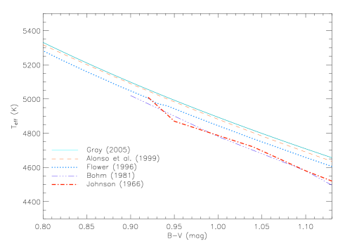
Figure 4: Examples of temperature calibrations published by several authors.

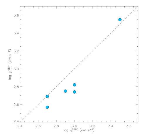
Figure 5: Photometric gravities vs. spectroscopic gravities derived by Pasquini et al. (2004) for the giant stars studied in IC 4651.

4.2.3 Reddening

To determine the reddening of IC 4651, we have used the $T_{\mathrm{eff}}-(B-V)$ calibrations of Gray (2005) and of Alonso et al. (1996, 1999), which includes the metallicity effect ([Fe/H]=0.10$\pm$0.03 for IC 4651, Pasquini et al. 2004). Deriving the intrinsic color index for all the stars from these relationships and comparing them with the observed colors, we obtain from the Gray’s calibration $E(B-V)=0.111\pm 0.018,0.164\pm 0.015$ and from the Alonso’s calibration $E(B-V)=0.127\pm 0.016,0.167\pm 0.017$, in which the two values correspond to the results obtained with the two temperatures $T_{\mathrm{eff}}^{\rm LDR}$ and $T_{\mathrm{eff}}^{\rm SPEC}$, respectively. The color excesses obtained with the two calibrations are very similar and this improves if one considers the effective temperatures $T_{\mathrm{eff}}^{\rm LDRc}$ derived by the LDR method and corrected for metallicity effects. In this case the color excesses obtained with $T_{\mathrm{eff}}^{\rm LDRc}$ is $E(B-V)=0.120\pm 0.016$, which is near to the value obtained considering the Alonso’s calibration. In addition, our color excess values are in good agreement with the results of $E(B-V)=0.15$, 0.10, 0.13, 0.10, 0.10 and 0.15 obtained by Eggen (1971), Nissen (1988), Kjeldsen & Frandsen (1991), Meibom et al. (2002), Anthony-Twarog & Twarog (2000) and Pasquini et al. (2004), respectively. Since Meibom et al. (2002), Anthony-Twarog & Twarog (2000) and Pasquini et al. (2004) compute $E(b-y)$, the relation $E(b-y)=0.72E(B-V)$ (Cardelli et al. 1989) has been used. These results seem to confirm our analysis of the Section 4.2.1 that the reddening value derived by Carretta et al. (2004) of $E(B-V)=0.083\pm 0.011$ is likely too low.

4.2.4 Mass and age

Since the PDF method allows us to derive complete probability distribution functions separately for each analysed stellar parameter, we have been able to derive the mass of the six stars studied in IC 4651 and the age of the cluster.

The results of the mass and age distributions based on the PDF method are plotted in Fig. 6 and listed in Table 2, both for the temperatures $T_{\mathrm{eff}}^{\rm LDR}$ and $T_{\mathrm{eff}}^{\rm SPEC}$. The mass and age distributions obtained for $T_{\mathrm{eff}}^{\rm LDRc}$ and $T_{\mathrm{eff}}^{\rm PHOT}$ are also shown for comparison.

We find that the average mass of the six giant stars studied in IC 4651 is 2.0$\pm$0.2 $M_{\sun}$. Pasquini et al. (2004) use stellar models of 1.8$M_{\sun}$ to reproduce the lithium abundances as a function of temperature simultaneously for ten post-turnoff and giant stars (see their Fig. 5). If we instead consider only the six giant stars, the lithium abundance after the dredge-up is $0.2\raisebox{-2.15277pt}{$\>\stackrel{{\scriptstyle\textstyle<}}{{\sim}}\>$}\log N(Li)\raisebox{-2.15277pt}{$\>\stackrel{{\scriptstyle\textstyle<}}{{\sim}}\>$}2.0$. This lithium abundance can be explained by means of a 2.0$M_{\sun}$ rotating model with initial rotational velocity $V_{\rm rot}$ of 110 km s^-1 and with a subsequent modest braking which leads to retain more lithium (Palacios et al. 2003). This mass value is consistent with our determination.

The cluster age found with the PDF method is 1.2$\pm$0.2 Gyr. This agrees with the value of $\log$(Age/yr)=9.15$\pm$0.05 ($1.40\pm 0.15$ Gyr) that we determined via isochrone fitting (Section 4.2.2), but is significantly lower than the values of 2.4$\pm 0.3$ Gyr and 1.7$\pm$0.15 Gyr found by Anthony-Twarog et al. (1988) and Meibom et al. (2002), respectively. Discussing the origin of these differences is beyond the scope of this paper. We just recall that the main differences between our and their isochrone fitting is that we consider also the position of the red clump in the CMD, additionally to the position of the main sequence and turn-off stars. The red clump provides a strong constraint to the apparent distance modulus that can be used in the isochrone fitting, thus better constraining the cluster age via the turn-off.

Clearly the errors associated to our ages and masses should be intended as internal errors. The fact of using different stars average out the errors on the single objects, however, all possible effects due, for instance, to a temperature scale shift and to the use of a particular set of evolutionary tracks are not considered. Systematic effects will change our results in a different way, depending on the position of the stars in the CMD. For instance, while the temperature is not of paramount importance in the Hertzsprung gap (star E95), it is the most critical parameter for Red Giant Branch stars. As far as the effective temperature scale is concerned, we tested the PDF method with the three stars 27, 76, and 146 studied by Carretta et al. (2004), with $T_{\rm eff}=4610,4620,4730$ K, $V=10\aas@@fstack{m}91,10\aas@@fstack{m}91,10\aas@@fstack{m}94$, respectively, and adopting their reddening ($E(B-V)=0.083$) and their apparent distance modulus ($V-M_{V}=$10.15). The results are that for the stars 27 and 76 we obtain masses and ages well out of the accepted range (Age$\sim 3.4$ Gyr, $M\simeq 1.3M_{\sun}$), while for the star 146 the result (Age$\sim 1.7$ Gyr, $M\simeq 1.8M_{\sun}$) is well compatible with our and within the range of the most accepted values avaliable in literature. This shows that while a shift of $\sim$100 K doesn’t change our analysis in a dramatic way, a difference of 200 K will produce unacceptable results.

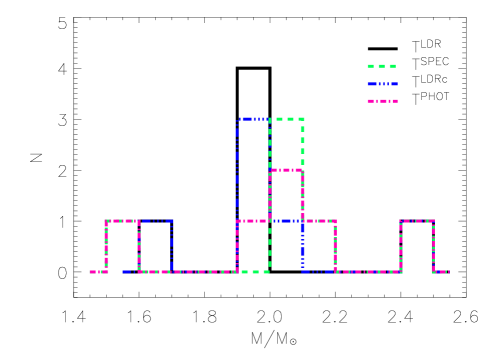
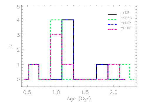
Figure 6: Mass and age distributions of the giant stars in IC 4651 for the different values of the effective temperature.

Table 2: Parameters of the giant stars analysed in IC 4651.

Name	$T_{\mathrm{eff}}^{\rm LDR}$	$T_{\mathrm{eff}}^{\rm SPEC}$	$T_{\mathrm{eff}}^{\rm LDRc}$	$M_{\rm V}$	$\log g^{\rm PHOT}$	$\log g^{\rm SPEC}$	$M^{\rm LDR}$	$M^{\rm SPEC}$	AgeLDR	AgeSPEC
	(K)	(K)	(K)	(mag)	(cm s-1)	(cm s-1)	($M_{\sun}$)	($M_{\sun}$)	(Gyr)	(Gyr)
E12	4926	5000	4945	0.524	2.50	2.7	2.464	2.496	0.698	0.662
E8	4821	4900	4840	0.867	2.63	2.7	2.018	2.156	1.197	0.999
E60	4833	4900	4852	1.070	2.69	2.9	2.013	2.064	1.175	1.096
E98	4806	4900	4825	1.080	2.66	3.0	1.984	2.061	1.218	1.098
MEI 11218	4906	5000	4925	1.259	2.75	3.0	2.027	2.069	1.115	1.044
E95	5482	5800	5501	2.153	3.47	3.5	1.690	1.582	1.779	2.166

5 Conclusions

In this work we have derived accurate atmospheric parameters for field stars and for six giant stars in the open cluster IC 4651.

For the former group of stars, with very low extinction and well determined physical parameters ($T_{\mathrm{eff}}$, $\log g$, $\xi$), we find a good agreement between the temperatures computed by da Silva et al. (2006) from spectral synthesis and those derived by us with the LDR technique. This gives strong support to the effectiveness of the LDR method in deriving effective temperatures.

For the giant stars in the intermediate-age open cluster IC 4651, the LDR method allowed us to determine accurate effective temperature values, overcoming the problem of parameters degeneracy (in $T_{\mathrm{eff}}$, $\log g$, $\xi$) encountered in the spectral synthesis method, and to derive the reddening of the cluster. We find that our value of $E(B-V)$ is in agreement with previous works (e.g., Pasquini et al. 2004), while it seems it has been underestimated by some other author (e.g., Carretta et al. 2004), who likely underestimated the stellar effective temperatures.

Thanks to the PDF method developed by Jørgensen & Lindegren (2005) and slightly modified in da Silva et al. (2006), we are able to find a mass of 2.0$\pm$0.2$M_{\sun}$ for the giant stars and a cluster age of 1.2$\pm$0.2 Gyr, by adopting the effective temperature derived with the LDR technique.

We conclude that our approach is well suitable to derive effective temperatures and reddening of evolved stars and clusters with a nearly solar-metallicity. The determination of very precise temperature is of great importance to derive stellar mass and age. For this reason, the LDR method could be inverted and used for stellar population studies in alternative and/or in addition to those based on photometric data.