Rigidity-dependent cosmic ray energy spectra in the knee region obtained with the GAMMA experiment

Abstract

On the basis of the extensive air shower (EAS) data obtained by the GAMMA experiment, the energy spectra and elemental composition of the primary cosmic rays are derived in the $10^{3}-10^{5}$ TeV energy range. The reconstruction of the primary energy spectra is carried out using an EAS inverse approach in the framework of the SIBYLL2.1 and QGSJET01 interaction models and the hypothesis of power-law primary energy spectra with rigidity-dependent knees. The energy spectra of primary $H,He,O$-like and $Fe$-like nuclei obtained with the SIBYLL interaction model agree with corresponding extrapolations of the balloon and satellite data to $\sim 10^{3}$ TeV energies. The energy spectra obtained from the QGSJET model show a predominantly proton composition in the knee region. The rigidity-dependent knee feature of the primary energy spectra for each interaction model is displayed at the following rigidities: $E_{R}\simeq 2500\pm 200$ TV (SIBYLL) and $E_{R}\simeq 3100-4200$ TV (QGSJET).
All the results presented are derived taking into account the detector response, the reconstruction uncertainties of the EAS parameters, and fluctuations in the EAS development.

, , , , ,

1 Introduction

The investigation of the energy spectra and elemental composition of primary cosmic rays in the knee region ($10^{3}-10^{5}$ TeV) remains one of the intriguing problems of modern high energy cosmic-ray physics. Despite the fact that these investigations have been carried out for more than half a century, the data on the elemental primary energy spectra at energies $E>10^{3}$ TeV still need improvement. The high statistical accuracies of recent EAS experiments [1, 2, 3, 4] have confirmed the presence of a bend in the all-particle primary energy spectrum at around $3\cdot 10^{3}$ TeV (called the ”knee”) from an overall spectrum $\propto E^{-2.7}$ below the knee to $\propto E^{-3.1}$ beyond the knee, and a change in composition toward heavier species with increasing energy in the $10^{3}-10^{5}$ TeV region. However, separating the primary energy spectra of elemental groups remains difficult, both due to uncertainties in the interaction model and the uncertainties associated with the solutions to the EAS inverse problem [5, 6].

One of the most studied class of models for the origin of cosmic rays in this energy region, which assumes that supernova remnants are their main source, predicts rigidity-dependent primary energy spectra in the knee region ([7, 8] and references therein). Other astrophysical models for the origin of the knee, such as Galactic propagation effects [9, 10] also predict rigidity-dependent spectra. Such energy spectra of primary nuclei with rigidity-dependent knees can approximately describe the observed EAS size spectra in the $10^{3}-10^{5}$ TeV energy region in the framework of conventional interaction models [11, 12, 13, 14, 15]. However, an alternative class of models predicts mass-dependent knees (see [16] and references therein for a recent review of models of the origin of the knee). In the present analysis, we will assume a rigidity-dependent knee; the appropriateness of this hypothesis will be briefly examined in the discussion section.

The GAMMA facility (Fig. 1) was designed at the beginning of the 1990’s in the framework of the ANI experiment [17] and the first results of EAS investigations were presented in [18, 19, 20, 21]. The main characteristic features of the GAMMA experiment are the mountain location, the symmetric location of the EAS detectors, and the underground muon scintillation carpet which detects the EAS muon component with energy $E_{\mu}>5$ GeV.

Here, a description of the GAMMA facility, the main results of investigation during 2002-2004 [20, 21, 22] and evaluations of primary energy spectra in the knee region are presented in comparison with the corresponding simulated data in the framework of the SIBYLL [23] and QGSJET [24] interaction models. Preliminary results have already been presented in [25, 26, 27].

2 GAMMA experiment

The GAMMA installation [18, 19, 20, 21, 22] is a ground-based array of 33 surface particle detection stations and 150 underground muon detectors, located on the south side of Mount Aragats in Armenia. The elevation of the GAMMA facility is 3200 m above sea level, which corresponds to 700 g/cm² of atmospheric depth. A diagrammatic layout is shown in Fig. 1.

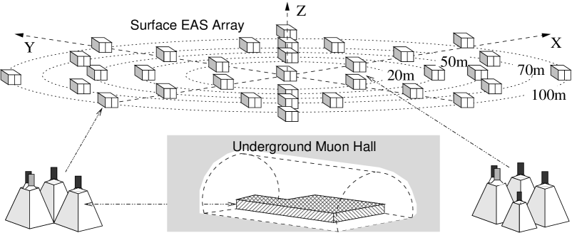
Figure 1: Diagrammatic layout of the GAMMA facility.

The surface stations of the EAS array are located on 5 concentric circles of radii $\sim$20, 28, 50, 70 and 100 m, and each station contains 3 square plastic scintillation detectors with the following dimensions: $1\times 1\times 0.05$ m³. Each of the central 9 stations contains an additional (4th) small scintillator with dimensions $0.3\times 0.3\times 0.05$ m³ (Fig. 1) for high particle density ($\gg 10^{2}$ particles/m²) measurements.
A photomultiplier tube is positioned on the top of the aluminum casing covering each scintillator. One of the three detectors of each station is examined by two photomultipliers, one of which is designed for fast timing measurements.
150 underground muon detectors (muon carpet) are compactly arranged in the underground hall under 2.3 kg/cm² of concrete and rock. The scintillator dimensions, casings and photomultipliers are the same as in the EAS surface detectors.

2.1 Detector system and triggering

The output voltage of each photomultiplier is converted into a pulse burst by a logarithmic ADC and transmitted to a CAMAC array, where the corresponding electronic counters produce a digital number (“code”) of pulses in the burst. Four inner (“trigger”) stations at a radius of 20m are monitored by a coincidence circuit. If at least two scintillators of each trigger station each detect more than 3 particles, the information from all detectors are then recorded along with the time between the master trigger pulse and the pulses from all fast-timing detectors. The given trigger condition provides EAS detections with an EAS size threshold $N_{ch}>(0.5-1)\cdot 10^{5}$ for a location of the EAS core within the $R<50$ m circle. The shower size thresholds for $100\%$ shower detection efficiency are equal to $N_{ch}=3\cdot 10^{5}$ and $N_{ch}=5\cdot 10^{5}$ for EAS core locations within $R<25$ m and $R<50$ m respectively [18].
Before being placed on the scintillator casing, all photomultipliers were tested by a test bench using a luminodiode method where the corresponding parameters of the logarithmic ADC and the upper limit ($(0.5-1)\cdot 10^{4}$) [28] of the particle density measurement ranges were determined for each detector. The number of charged particles ($n_{i}$) passing through the i-th scintillator is calculated using a logarithmic transformation: $\ln n_{i}=(C-C_{0})/d$ [28], where the scale parameter $d\simeq(9-10)\pm 0.35$ is determined for each detector by the test bench, $0\leq C\leq 2^{7}-1$ is the output digital code from the CAMAC array corresponding to the energy deposit of $n$ charged particles into the scintillator, and $C_{0}\simeq(5-6)\pm 0.25$ is equal to the mode of the background single particle digital code spectra (Section 2.4). The time delay is estimated by the pair-delay method [29] to give a time resolution of about $4-5$ ns.

2.2 Reconstruction of EAS parameters

The EAS zenith angle ($\theta$) is estimated on the basis of the shower front arrival times measured by the 33 fast-timing surface detectors, applying a maximum likelihood method and the flat-front approach [29, 30]. The corresponding uncertainty was tested by Monte Carlo simulations and is equal to $\sigma(\theta)\simeq 1.5^{\circ}$ [18]. The reconstruction of the EAS size ($N_{ch}$), shower age ($s$) and core coordinates ($x_{0},y_{0}$) is performed based on the Nishimura-Kamata-Greisen (NKG) approximation to the measured charged particle densities ($\{n_{i}\},i=1,\dots,m$), using $\chi^{2}$ minimization to estimate $x_{0},y_{0}$ and a maximum likelihood method to estimate $N_{ch}$, taking into account the measurement errors. Gamma-quanta conversions in the scintillator and housing were taken into account in the estimates of $N_{ch}$ (Section 2.3).
The logarithmic transformation $L(n_{i})=\ln n_{i}-(1/m)\sum\ln n_{i}$ for $n_{i}\neq 0$ enables an analytical solution for the EAS age parameter ($s$) using $\chi^{2}$ minimization [30, 31]. Unbiased ($<5\%$) estimations of $N_{ch},s,x_{0}$ and $y_{0}$ shower parameters are obtained for $N_{ch}>5\cdot 10^{5}$, $0.3<s<1.6$, $\theta<30^{\circ}$ and distances $R<25$ m from the shower core to the center of the EAS array. The shower age parameter ($s$) is estimated from the surface scintillators located inside a $7$ m $<R_{i}<80$ m ring area around the shower core (Section 2.3).
The EAS detection efficiency ($P_{d}$) and corresponding accuracies are derived from mimic shower simulations taking into account the EAS fluctuations and measurement errors (Section 2.4) and are equal to: $P_{d}=100\%$, $\Delta N_{ch}/N_{ch}\simeq 0.1$, $\Delta s\simeq 0.05$, $\Delta x$ and $\Delta y\simeq 0.5-1$ m. These results were also checked with CORSIKA [32] simulated EAS (Section 2.3) and depend slightly on shower core location for $R<50$ m.
The reconstruction of the total number of EAS muons ($N_{\mu}$) from the detected muon densities ($\{n_{\mu,j}\},j=1,\dots,150$) in the underground muon hall is carried out by restricting the distance to $R_{\mu}<50$ m from the shower core (the so-called EAS “truncated” muon size [18, 33]) and using the approximation to the muon lateral distribution function [18, 34]: $\rho_{\mu}(r)=cN_{\mu}(R_{\mu}<50{\rm m})\exp{(-r/r_{0})}/(r/r_{0})^{0.7}$, where $r_{0}=80$ m [35] and $c=1/2\pi\int_{0}^{50}\rho(r)rdr$. The EAS truncated muon size $N_{\mu}(R_{\mu}<50{\rm m})$ is estimated at known (from the EAS surface array) shower core coordinates in the underground muon hall. Unbiased estimations for muon size are obtained for $N_{\mu}>10^{3}$ using a maximum likelihood method and assuming Poisson fluctuations in the detected muon numbers. The reconstruction accuracies of the truncated muon shower sizes are equal to $\Delta N_{\mu}/N_{\mu}\simeq 0.2-0.35$ at $N_{\mu}\simeq 10^{5}-10^{3}$ respectively.
It should be noted that the detected muons in the underground hall are always accompanied by the electron-positron equilibrium spectrum which is produced when muons pass through the matter (2300 g/cm²) over the scintillation carpet; this is taken into account in our results (Section 3.2).

2.3 Detector response

The GAMMA detector response taking into account the EAS $\gamma$-quanta contribution was computed by EAS simulations using the CORSIKA 6.031 code [32] (NKG and EGS modes, GHEISHA2002) with the QGSJET01 [24] and SIBYLL 2.1 [23] interaction models for 4 types ($A\equiv H,He,O,Fe$) of primary nuclei. Each EAS particle ($\gamma,e,\mu,h$) obtained from CORSIKA (EGS mode) at the observation level was examined by passing through the steel casing (1.5 mm) of the detector station and then through the corresponding scintillator. The pair production and Compton scattering processes were additionally simulated in the case of EAS $\gamma$-quanta. The resulting energy deposit in the scintillator was converted to an ADC code and inverse-decoded into a number of “detected” charged particles taking into account all uncertainties of the ADC parameters ($C_{0},d$) and fluctuations in the light collected by the photomultipliers ($\sigma_{l}\simeq 0.25/\sqrt{n}$).
Using the simulation scenario above, 200 EAS events with shower size threshold $N_{ch}>5\cdot 10^{5}$ were simulated with CORSIKA simultaneously in the EGS and NKG modes for each of the $A\equiv H,He,O$ and $Fe$ primary nuclei, with logarithm-uniform energy spectra in the $10^{3}-10^{5}$ TeV energy range. The computation of the charged particle densities in surface detectors in the NKG mode was performed by applying two-dimensional interpolations of the corresponding shower electron (and positron) density matrix from CORSIKA [32], along with the individual EAS muons and hadrons.

Figure 2: Biases (a) and standard deviations (b) versus EAS size, and distributions of biases in shower size (c) and shower age parameter (d) for the SIBYLL (circle symbols, lines) and QGSJET (square symbols) interaction models for primary $H$ (empty symbols, solid lines) and $Fe$ (filled symbols, dashed lines) nuclei.

A $\sim 5\%$ agreement between the EGS (including the EAS $\gamma$-quanta contribution) and NKG simulated EAS data was attained for an $E_{e}\simeq 1$ MeV kinetic energy threshold of shower electrons (and positrons) in the NKG mode, considering only the 7m $<R_{i}<80$m ring area used in the determination of the shower age parameter. Thus the underestimation of the EAS particle density due to the threshold of the detected energy deposit ($E_{d}\simeq 8$ MeV [18, 25]) in the scintillators is compensated by the EAS $\gamma$-quanta contribution.
The corresponding biases

$$\delta_{N_{ch}}(A,N_{ch})\equiv\frac{N_{ch}(E_{e}=1{\rm\,MeV},NKG)}{N_{ch}(E_{d},\gamma,EGS)}$$

and standard deviations $\sigma(\delta_{N_{ch}})$ versus the reconstructed EAS size ($N_{ch}$) are shown in Fig. 2 (a) and (b) respectively, for the SIBYLL (circle symbols) and QGSJET (square symbols) interaction models and for primary $H$ (empty symbols) and $Fe$ nuclei (filled symbols). The distributions of the biases in reconstructed EAS sizes ($\delta_{N_{ch}}$) and shower age parameters

$$\delta_{s}(A)\equiv s(E_{e}=1{\rm\,MeV},NKG)-s(E_{d},\gamma,EGS)$$

are shown in Fig. 2 (c) and (d) respectively, for a shower size threshold $N_{ch}>5\cdot 10^{5}$, the SIBYLL interaction model, and primary $H$ (solid lines) and $Fe$ (dashed lines) nuclei.
The observed ($\sim 5\%$) biases in $\delta_{N_{ch}}$ (Fig. 2a) for the 4 kinds of primary nuclei depend only weakly on the interaction model ($\leq 5\%$) and zenith angles ($\leq 3\%$ for $\theta<30^{\circ}$), and the biases in age parameter $\delta_{s}$ can be considered negligible. The NKG-mode simulated sizes were divided by the estimated biases $\delta_{N_{ch}}(A,N_{ch})$ in the reconstruction of the primary energy spectra (Section 3.1).

2.4 Measurement errors and density spectra

The close disposition of the $k=1,2,3$ scintillators in each of the ($i$-th) detector stations of the GAMMA surface array enables a calibration of the measurement error using the detected EAS data. The measured and simulated particle density discrepancies $(n_{k}-\rho)/\rho$ versus the average value $\rho=(1/3)\sum{n_{k}}$ for distances $R_{i}>10$ m from the shower core are shown in Fig. 3 (circle symbols), and are completely determined by Poisson fluctuations (at $R_{i}\gg 1$ m ) and the measurement errors.

Figure 3: Particle density discrepancies (circle symbols) and measurement error for a single detector (square symbols) versus charged-particle density.

The agreement between the measured and simulated dependences enables the extraction of the actual measurement errors of the GAMMA detectors. The corresponding results, obtained from the simulations without Poisson fluctuations, are shown in Fig. 3 (square symbols).
The background omni-directional single particle spectra (in units of ADC code) detected by GAMMA surface scintillators in 78 s of operation time are shown in Fig. 4 (dotted lines). The background single particle spectra detected by underground

Figure 4: Background single particle spectra of 15 surface detectors (dotted lines). The symbols (solid line) are the expected spectra taking into account (without) measurement errors.

muon scintillators have the same shape but about 10 times lower intensities. These spectra (pulse height distributions) along with the known zenith angle distributions and composition ($\sim 40\%e,50\%\mu$) of the background charged particles at the observation level [36] are used for the operative determination of the ADC parameters ($C_{0}$) for each experimental run. The symbols and solid lines in Fig. 4 display the corresponding expected spectra obtained by CORSIKA (EGS) simulation, without errors (solid line) and taking into account the measurement errors (symbols) respectively. The minimal primary energy in the simulation of the background particle spectra was determined by the 7.6 GV geomagnetic rigidity cutoff in Armenia.
Because the effective primary energies responsible for the single particle spectra at the observation level of 700 g/cm² are around $100$ GeV, and this energy range has been studied by direct measurements in balloon and satellite experiments, the primary energy spectra and elemental composition in the Monte Carlo simulation were taken from power-law approximations to the direct measurement data [37]. It should be noted that the expected single particle spectra at these energies are practically the same for the QGSJET and SIBYLL interaction models, because most of the interactions occur in the energy range where accelerator data are used.
Fig. 5 (symbols) displays the EAS charged particle density spectra measured by the surface detectors (left panel) and underground muon detectors (right panel) at $R_{i}<50$ m with different EAS size thresholds: $N_{ch}>5\cdot 10^{5}$, $N_{ch}>10^{7}$ (and additionally $N_{ch}>2\cdot 10^{6}$ for the muon density spectra).

Figure 5: Detected (symbols) and expected (lines) particle density spectra measured by the surface scintillators (left panel) and underground muon scintillators (right panel).

The showers were selected with $\theta<30^{\circ}$ and shower core location in the $R<25$ m range from the center of the GAMMA facility (Fig. 1). The corresponding expected spectra (lines) for different interaction models are also shown in Fig. 5. The primary energy spectra and elemental composition for these simulations were those obtained in the combined approximation solution to the EAS inverse problem (Section 3.3). There is good agreement between the expected and observed data for the surface array over the full measurement range (about four orders of magnitude). However, agreement of the detected muon density spectra with the expected ones is attained only in the $N_{ch}<10^{7}$ range. The observed discrepancies for the muon density spectra at $N_{ch}>10^{7}$ are unaccounted for at present, and will require subsequent investigations.

2.5 EAS data set

The data set analyzed in this paper was obtained over $6.19\cdot 10^{7}$ s of operating live time of the GAMMA facility, from 2002 to 2004. Showers were selected for analysis with the following criteria: $N_{ch}>5\cdot 10^{5}$, $R<25$ m, $\theta<30^{\circ}$, $0.3<s<1.6$, $\chi^{2}(N_{ch})/m<3$ and $\chi^{2}(N_{\mu})/m<3$ (where $m$ is the number of scintillators with non-zero signal), yielding a total data set of $1.9\cdot 10^{5}$ selected showers.

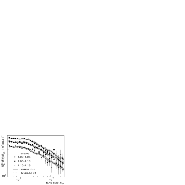
Figure 6: EAS size spectra for 3 zenith angle intervals (symbols) and corresponding expected spectra according to the SIBYLL (solid lines) and QGSJET (dashed lines) interaction models.

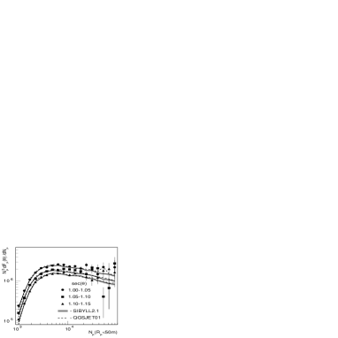
Figure 7: Normalized EAS truncated muon size spectra for 3 zenith angle intervals (symbols) and corresponding expected spectra for the SIBYLL (solid lines) and QGSJET (dashed lines) interaction models.

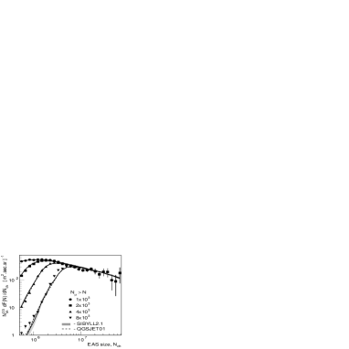
Figure 8: EAS size spectra (symbols) for different truncated muon size thresholds ($N_{\mu}$) and corresponding expected spectra according to the SIBYLL (solid lines) and QGSJET (dashed lines) interaction models.

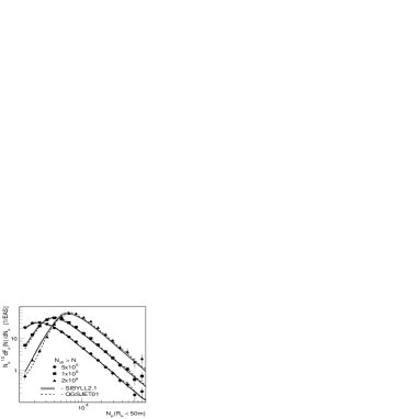
Figure 9: Normalized EAS truncated muon size spectra (symbols) for different shower size thresholds ($N_{ch}$) and corresponding expected spectra according to the SIBYLL (solid lines) and QGSJET (dashed lines) interaction models.

The selected measurement range provided $100\%$ EAS detection efficiency (Section 2.2) and similar conditions for the reconstruction of the shower lateral distribution functions.
The measured variable distributions used in the combined approximation approach to the EAS inverse problem (Section 3.3) are shown in Figs. 6–11 (symbols). All lines and shaded areas in these figures correspond to the expected spectra computed on the basis of the EAS inverse problem solution in the framework of the SIBYLL and QGSJET interaction models. These expected (forward folded) spectra are computed by Monte-Carlo integration (Section 3.1) using the simulated EAS database, which results in the statistical fluctuations evident in many of these predicted spectra.

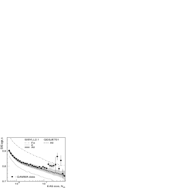
Figure 10: Dependence of the average EAS age parameter on EAS size (symbols) along with expected values for the SIBYLL (solid line) and QGSJET (dashed line) interaction models. The dotted and dash-dotted lines correspond to expected values for primary hydrogen and iron nuclei, respectively, for the SIBYLL interaction model.

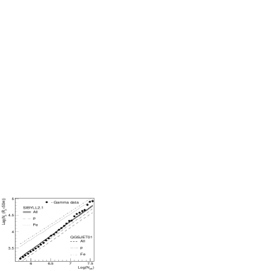
Figure 11: Average EAS truncated muon size $N_{\mu}$ versus EAS size $N_{ch}$ (symbols). The lines and shaded area are the expected dependences for the SIBYLL and QGSJET interaction models and primary $p$, $Fe$ and mixed (Table 1) compositions.

The EAS size spectra ($N^{2.5}_{ch}\cdot\d F(\theta)/\d N_{ch}$) for three zenith angle intervals are shown in Fig. 6. The EAS truncated muon size spectra in the same zenith angle intervals are shown in Fig. 7; these spectra are normalized per unit shower with $N_{ch}>5\cdot 10^{5}$ and $\theta<30^{\circ}$. The EAS size spectra for $\theta<30^{\circ}$ and different thresholds in EAS truncated muon size are shown in Fig. 8. The normalized EAS truncated muon size spectra for different EAS size thresholds are shown in Fig. 9. Fig. 10 displays the dependence of the average EAS age parameter on EAS size $s(N_{ch})$. Fig. 11 shows the observed $N_{\mu}(N_{ch})$ dependence and the corresponding expected values for primary proton, iron and mixed ($p,He,O,Fe$, Section 3.3) compositions computed in the framework of the SIBYLL and QGSJET interaction models.

3 EAS inverse problem and primary energy spectra

3.1 Key assumptions

The observed spectra $F(\mathbf{q})$ of the measured EAS parameters $\mathbf{q}=(N_{ch},N_{\mu},s)$ result from convolutions of the energy spectra $I_{A}(E)$ of primary nuclei ($A\equiv H,He,\dots$ at least up to $Ni$) with the probability density distributions $W_{A}(E,\mathbf{q})$ [13, 33, 40]:

$$F(\mathbf{q})=\sum_{A}\int_{E}W_{A}(E,\mathbf{q})I_{A}(E)\d E\;.$$ (1)

The functions $W_{A}(E,\mathbf{q})$ are derived using a model of the EAS development in the atmosphere and convolution of the resulting shower spectra at the observation level with the corresponding response functions [6, 25].
The integral equation (1) defines the EAS inverse problem, namely the evaluation of the primary energy spectra $I_{A}(E)$ on the basis of the measured distributions $F(\mathbf{q}_{i})$ (in $i=1,\dots,V$ discrete bins) and the known kernel functions $W_{A}(E,\mathbf{q}_{i})$ [6, 25, 40]. The multidimensional kernel functions $W_{A}(E,\mathbf{q})$ can be computed using interpolations [13] or approximations [6] to the corresponding spectra, which are previously obtained by CORSIKA EAS simulations in the framework of a given interaction model, for different groups of primary nuclei and a set of primary energies and zenith angles.

In the present work, the computations of the expected shower spectra (forward folding) from (1) for given primary energy spectra $I_{A}(E)$ are performed by Monte Carlo integration [42, 43], using an arbitrary positive weight function $I_{0}(A,E)$ determined in the same domain as the primary spectra $I_{A}(E)$ and normalized such that $\int W_{A}(E)I_{0}(A,E)\d E=1$.
Multiplying and dividing the integrand in (1) by $I_{0}(A,E)$, expression (1) is converted to the form:

$$F(\mathbf{q}_{i})=\sum_{A}\Big{<}\frac{I_{A}(E)}{I_{0}(A,E)}\Big{>}_{\mathbf{q}_{j}\in\mathbf{q}_{i}}\;.$$ (2)

The averaging in (2) is performed over random $E_{j}$ ($j=1,\dots,\mathcal{N_{A}}$) distributed with a probability density function $I_{0}(A,E)W_{A}(E\mid\mathbf{q}_{j}\in\mathbf{q}_{i})$, with shower parameters $\mathbf{q}_{j}$ within the given $\mathbf{q}_{i}$ bin. The reconstructed shower parameters $\mathbf{q}_{j}(A,E_{j})$ are obtained by EAS simulations in the framework of a given interaction model, taking into account the corresponding response functions $<\delta_{N_{ch}}(A,N_{ch})>$ (Section 2.3).
As a weight function we chose the power law spectrum $I_{0}(A,E)\propto E^{-1.5}$ which provides an accuracy for integration $\Delta F/F\simeq 1/\sqrt{\mathcal{N}}$ and relatively small statistical errors for the simulated EAS samples both within and especially beyond the knee region. The accuracy of Monte-Carlo integration with this weight function was checked using power-law spectra $f(x)\propto x^{-\gamma}$ with $\gamma=2.5-3.3$ and log-normal distributions $W(x,y)$, and found to be adequate for our purposes.

In order to evaluate the primary energy spectra on the basis of the EAS data set we regularized the integral equation (1) using a parametrization method [13, 15]. The solutions for the primary energy spectra in (1) were sought based on a broken power-law function with a “knee” at the rigidity-dependent energy $E_{k}(A)=E_{R}\cdot Z$, and the same spectral indices for all species of primary nuclei ($A\equiv p,He,O,Fe$), $\gamma_{1}$ below and $\gamma_{2}$ above the knee respectively:

$$\frac{\d I_{A}}{\d E}=\Phi_{A}\,\left(\frac{E_{k}}{1\,{\rm TeV}}\right)^{-\gamma_{1}}\left(\frac{E}{E_{k}}\right)^{-\gamma}\>,$$ (3)

where $\gamma=\gamma_{1}$ for $E\leq E_{k}(A)$, $\gamma=\gamma_{2}$ for $E>E_{k}(A)$, $E_{R}$ is the particle’s magnetic rigidity and $Z$ the charge of nucleus $A$.
The integral equation (1) is thereby transformed into a parametric equation with the unknown spectral parameters $\Phi_{A},E_{R},\gamma_{1}$ and $\gamma_{2}$, which are evaluated by minimization of the $\chi^{2}$ function:

$$\chi^{2}=\sum_{u=1}^{U}\sum_{i=1}^{V_{u}}\frac{(\zeta_{u,i}-\xi_{u,i})^{2}}{\sigma^{2}(\zeta_{u,i})+\sigma^{2}(\xi_{u,i})}\;,$$ (4)

where $U$ is the number of examined functions $\zeta_{u,i}\equiv F_{u}({q}_{u,i})$ obtained from the experimental data with statistical accuracies $\sigma(\zeta_{u,i})$ in $i=1,\dots,V_{u}$ bins, and $\xi_{u,i}$ and $\sigma(\xi_{u,i})$ are the corresponding expected (forward folded) values from (2) and their (statistical) uncertainties.

3.2 Simulated EAS database

EAS simulations for the evaluation of the primary energy spectra using the GAMMA facility EAS data were carried out for $\mathcal{N}_{A}\equiv$ $10^{5}$ primary $H$, $7.1\cdot 10^{4}$ $He$, $4.6\cdot 10^{4}$ $O$ and $4.8\cdot 10^{4}$ $Fe$ nuclei using the CORSIKA NKG mode and the SIBYLL interaction model. The corresponding statistics for the QGSJET interaction model were: $10^{5}$, $6\cdot 10^{4}$, $4.4\cdot 10^{4}$ and $4\cdot 10^{4}$.
The energy thresholds of the primary nuclei were the same for both interaction models and were set at $E_{A,\min}\equiv 0.5,0.7,1$ and $1.2$ PeV for $H$, $He$, $O$ and $Fe$ respectively, and the upper energy limit was set at $E_{\max}=5\cdot 10^{3}$ PeV. The simulated energies were distributed following a weight function $I_{0}(A,E)\propto E^{-1.5}$, as explained above. The simulated showers had core coordinates distributed uniformly within a radius $R<25$ m, and zenith angles $\theta<30^{\circ}$. This ignores the effect of showers with true core coordinates outside the selection radius which have reconstructed coordinates with $R<25$ m; due to the good core reconstruction accuracy of $0.5-1$ m (Section 2.2), this effect may be neglected for our purposes.
All the EAS muons with energies of $E_{\mu}>4$ GeV at the GAMMA observation level were passed through the 2.3 kg/cm² of rock to the muon scintillation carpet (the underground muon hall). The fluctuations in the muon ionization losses, and the electron (and positron) accompaniment due to the muon electromagnetic and photonuclear interactions in the rock were taken into account, using the approximation of an equilibrium accompanying charged particle spectrum obtained from preliminary simulations with the FLUKA code [41] in the $0.005-20$ TeV muon energy range. The resulting charged particle accompaniment per EAS muon in the underground hall is equal to $0.06\pm 0.01$ ($100\%e$) and $11.0\pm 1.5$ ($98.5\%e,1.4\%h,0.04\%\mu$) at muon energies $0.01$ TeV and $10$ TeV respectively.
The total number of simulated EAS in the database were $\mathcal{N}=\sum\mathcal{N}_{A}\simeq 2.65\cdot 10^{5}$ EAS for the SIBYLL and $\mathcal{N}\simeq 2.44\cdot 10^{5}$ EAS for the QGSJET model.

3.3 Combined approximations to the EAS data

Using the aforementioned formalism (Section 3.1), the $U=6$ examined functions shown in Figs. 6–11 and the corresponding EAS data set, the unknown spectral parameters $\Phi_{A},E_{R},\gamma_{1}$ and $\gamma_{2}$ of parametrization (3) were derived by minimization of the $\chi^{2}$ (4) and forward folding (2), with a number of degrees of freedom $n_{d.f.}=\sum_{1}^{6}{V_{u}}-p-1\simeq 350$, where $p=7$ is the number of adjustable parameters.
The values of the spectral parameters (3) derived from the solution of the parameterized equation (1) are presented in Table 1 for the SIBYLL and QGSJET interaction models.

Table 1: Parameters of the primary energy spectra (3) from combined approximations to the EAS data. The scale factors $\Phi_{A}$ and particle rigidity $E_{R}$ respectively have units of (m${}^{2}\cdot$ s $\cdot$ sr $\cdot$ TeV)^-1 and TV.

Parameters	SIBYLL	QGSJET
$\Phi_{H}$	$0.095\pm 0.008$	$0.165\pm 0.005$
$\Phi_{He}$	$0.100\pm 0.012$	$0.020\pm 0.008$
$\Phi_{O}$	$0.034\pm 0.007$	$0.008\pm 0.004$
$\Phi_{Fe}$	$0.024\pm 0.004$	$0.013\pm 0.005$
$E_{R}$	$2500\pm 200$	$3200\pm 150$
$\gamma_{1}$	$2.68\pm 0.015$	$2.66\pm 0.010$
$\gamma_{2}$	$3.19\pm 0.03$	$3.11\pm 0.02$
$\chi^{2}/n_{d.f.}$	$2.0$	$1.5$

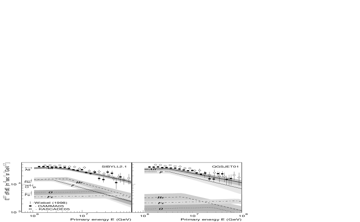
Figure 12: Energy spectra and abundances of the primary nuclei groups (lines and shaded areas) for the SIBYLL (left panel) and QGSJET (right panel) interaction models. All-particle spectra from GAMMA [27] and KASCADE [6] are shown as symbols. Vertical bars show the extrapolations of balloon and satellite data [37].

The primary energy spectra obtained for $p,He,O,$ and $Fe$ nuclei, along with the all-particle energy spectra, are shown in Fig. 12 (lines and shaded areas) for the SIBYLL (left panel) and QGSJET (right panel) interaction models. The symbols in Fig. 12 show the all-particle spectra obtained by KASCADE [6] from a 2-dimensional ($N_{e},N_{\mu}$) unfolding using an iterative method, and from GAMMA [27] using an event-by-event method. Also shown as error bars in the left panel of Fig. 12 are extrapolations of the balloon and satellite data to the energy $E\simeq 10^{6}$ GeV, computed using power-law approximations to the available direct measurement data [37]; these remain in reasonable agreement with more recent balloon experiment data [38, 39]. In this extrapolation, the $O$-like group was assumed to include the elements $Z=3$–16, and the $Fe$-like group the elements $Z=17$–28.
The expected EAS spectra and $N_{ch}(s)$ and $N_{ch}(N_{\mu})$ dependencies according to the solutions presented above are shown in Figs. 6–11 for the QGSJET (dashed lines) and SIBYLL (solid lines and shaded areas) interaction models. The vertical widths of the shaded areas correspond to the error bars of the expected spectra, which are comparable for the two interaction models.
It should be noted that the results obtained in the framework of the QGSJET interaction model strongly depend on the number of examined functions, which is not the case with the SIBYLL model.

3.4 2-Dimensional approach

Using (1), parametrization (3) and the 2-dimensional EAS spectra

$$F(\mathbf{q})\equiv\frac{\d^{2}F}{\d N_{ch}\d N_{\mu}}$$

we evaluated the parameters of the primary energy spectra by minimization of the corresponding $\chi^{2}$ function (4), with $U=1$. The computations were carried out with bin dimensions $\Delta\ln{N_{ch}}=0.15$ and $\Delta\ln{N_{\mu}}=0.25$, for $\theta<30^{\circ}$ and $N_{ch}>5\cdot 10^{5}$. The resulting number of degrees of freedom ($n_{d.f.}$) for the $\chi^{2}$ minimization was equal to about 240.
The best-fit spectral parameters and corresponding values of $\chi^{2}/n_{d.f.}$ for both interaction models are presented in Table 2.

Table 2: Parameters of the primary energy spectra (3) from 2-dimensional approximations to the EAS data. The scale factors $\Phi_{A}$ and particle rigidity $E_{R}$ respectively have units of (m${}^{2}\cdot$ s $\cdot$ sr $\cdot$ TeV)^-1 and TV.

Parameters	SIBYLL	QGSJET
$\Phi_{H}$	$0.109\pm 0.006$	$0.198\pm 0.006$
$\Phi_{He}$	$0.095\pm 0.006$	$0.028\pm 0.005$
$\Phi_{O}$	$0.050\pm 0.006$	$0.031\pm 0.002$
$\Phi_{Fe}$	$0.017\pm 0.002$	$0.006\pm 0.002$
$E_{R}$	$2500\pm 200$	$4200\pm 300$
$\gamma_{1}$	$2.70\pm 0.005$	$2.71\pm 0.030$
$\gamma_{2}$	$3.23\pm 0.08$	$3.23\pm 0.09$
$\chi^{2}/n_{d.f.}$	$1.2$	$1.3$

The contributions to the total $\chi^{2}$ from each 2-dimensional bin $\mathbf{q}_{i}=(N_{ch},N_{\mu})$ at the minimum of the $\chi^{2}$ function are shown in Figs. 13 and 14, for the SIBYLL and QGSJET models respectively.

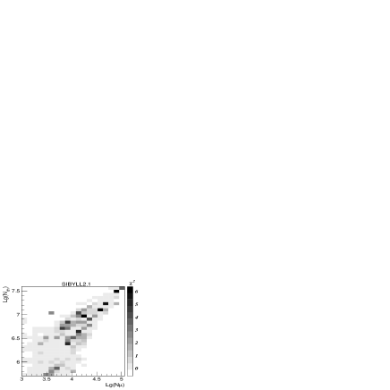
Figure 13: Contributions to the total $\chi^{2}$ from each ($N_{ch},N_{\mu}$) bin, for the SIBYLL interaction model.

Figure 14: Same as Fig. 13 for the QGSJET interaction model.

3.5 4-Dimensional approach

The amount of information about the primary energy spectra contained in the 4-dimensional spectrum of measured parameters

$$F(\mathbf{q})\equiv\frac{\d^{4}F}{\d N_{ch}\d N_{\mu}\d s\d\cos\theta}$$

is obviously always greater than the information contained in the 2-dimensional ($N_{ch},N_{\mu}$) spectrum (Section 3.4) or the cumulative amount of information contained in the combined spectra (Section 3.3). The main difference with the latter case is due to the inter-correlations between EAS parameters, which can only be fully taken into account in such a 4-dimensional approach.

Table 3: Parameters of the primary energy spectra (3) from the 4-dimensional analysis of the EAS data. The scale factors $\Phi_{A}$ and particle rigidity $E_{R}$ respectively have units of (m${}^{2}\cdot$ s $\cdot$ sr $\cdot$ TeV)^-1 and TV.

Parameters	SIBYLL	QGSJET
$\Phi_{H}$	$0.110\pm 0.004$	$0.190\pm 0.002$
$\Phi_{He}$	$0.091\pm 0.004$	$0.023\pm 0.003$
$\Phi_{O}$	$0.045\pm 0.004$	$0.038\pm 0.002$
$\Phi_{Fe}$	$0.030\pm 0.002$	$0.010\pm 0.002$
$E_{R}$	$2300\pm 230$	$3100\pm 200$
$\gamma_{1}$	$2.67\pm 0.005$	$2.68\pm 0.005$
$\gamma_{2}$	$3.13\pm 0.06$	$3.10\pm 0.06$
$\chi^{2}/n_{d.f.}$	$2.1$	$2.1$

On the basis of this 4-dimensional representation of the EAS data set, the simulated EAS database, and parameterization (3), equation (1) was solved by $\chi^{2}$ minimization, with $U=1$. The computations were carried out with the following bin dimensions: $\Delta\ln{N_{ch}}=0.15$, $\Delta\ln{N_{\mu}}=0.25$, $\Delta\sec{\theta}=0.05$, and $\Delta s=0.15$ on the left and right hand side of $s^{*}=0.85$ and $\Delta s=0.3$ elsewhere. The number of degrees of freedom in this 4-dimensional approximation was equal to $1640$. The values of spectral parameters (3) resulting from the solution of the parameterized equation (1) are presented in Table 3 for the QGSJET and SIBYLL interaction models.

4 Discussion

As can be seen from Fig. 12 and Tables 1–3, the derived primary energy spectra depend significantly on the interaction model, and slightly on the approach (Sections 3.2–3.5) applied to solve the EAS inverse problem. The derived abundances of primary nuclei at an energy $E\sim 10^{3}$ TeV in the framework of the SIBYLL model agree (in the range of 1-2 standard errors) with the corresponding extrapolations of the balloon and satellite data [37], whereas the results derived with the QGSJET model point toward a dominantly proton primary composition in the $10^{3}-10^{5}$ TeV energy range.
Although the derived formal accuracies of the spectral parameters in Tables 1–3 are high, the corresponding $\chi^{2}$ values are large, which demands further discussion. These large $\chi^{2}$ values do not necessarily imply disagreement between the EAS data and the derived primary energy spectra, but could be due to a number of other possible causes. We believe that the most likely causes of the large $\chi^{2}$ values of our spectral fits are systematic uncertainties related to the EAS simulations, in the interaction model or in the computation of the detector response (Section 2.3), and to the representation of the full cosmic ray composition by a small number of simulated nuclear species. We note that the inclusion of additional errors of about $5-7\%$ in the $\chi^{2}$ functions (4) will decrease the $\chi^{2}/n_{d.f.}\simeq 2$ in Tables 1–3 to $\chi^{2}/n_{d.f.}\simeq 1$.
We discuss in turn below a number of other possible causes and related issues, especially the possibility that our spectral parametrization is incorrect, in terms of the rigidity-dependent knee energy or common spectral index. We also consider briefly the uncertainties in the reconstructed spectral parameters, discuss possible issues with the convergence of the unfolding method and the number of elemental groups, and present some consistency checks on the simulated and experimental databases.

4.1 Rigidity-dependent knee hypothesis

A test of the spectral parametrization (3) was performed by evaluating the knee energies $E_{k}(A)$ independently for each primary nucleus $A\equiv H,He,O,Fe$ simultaneously with the spectral parameters $\Phi_{A}$,$\gamma_{1}$ and $\gamma_{2}$, using the combined approximation method described above (Section 3.3). The derived scale factors $\Phi_{A}$ and spectral indices $\gamma_{1}$ and $\gamma_{2}$ agreed with the data from Table 1 within errors, but they had somewhat larger uncertainties (typically by factors $\simeq 1.2-1.7$). The derived knee energies versus nuclear charge ($Z$) are shown in Fig. 15 for the SIBYLL and QGSJET interaction models (symbols), along with the corresponding expected values (lines) according to the rigidity-dependent knee hypothesis from Table 1.

Figure 15: Knee energies for each group of nuclei (symbols) versus nuclear charge $Z$. The expected values in the rigidity-dependent (thick lines) and mass-dependent (thin lines) knee hypotheses are also shown, for the QGSJET (dashed lines) and SIBYLL (solid lines) interaction models.

It can be seen from Fig. 15 that the independently adjusted knee energies agree with the rigidity-dependent knee hypothesis.
We also examined the alternative mass-dependent knee hypothesis; also shown as lines in Fig. 15 are the results of spectral fits using combined approximations (Section 3.3), in which the hypothesis $E_{k}(A)=E_{k}\cdot A$, with $A$ the nuclear mass, was assumed. The values of the $\chi^{2}_{\min}$ were practically the same as in Table 1, but the derived value of the spectral parameter $\gamma_{1}$ tended to the range $2.59\pm 0.02$, which is somewhat hard relative to expectations from the balloon and satellite data [37, 38, 39]. Within the uncertainties of our present analysis, our data are not in contradiction with this $A$-dependent knee hypothesis; however, it clearly does not yield a better agreement than our assumed rigidity-dependent hypothesis.

4.2 Common spectral index hypothesis

We attempted to similarly examine the possibility of independent spectral indices $\gamma_{1,A}$ for each primary nucleus, $A\equiv H,He,O,Fe$, but in that case encounter a difficulty. The solution found by $\chi^{2}$ minimization when these parameters are independent strongly depends on the initial values given to the minimization algorithm, making a thorough exploration of the multi-dimensional parameter space impractical, and the results inconclusive.
Figure 16 shows the $\chi^{2}(\gamma_{1})$ dependences for different spectral hypotheses. The thick solid line represents the $\chi^{2}(\gamma_{1})$ for parameterization (3), where the spectral index is common to all primary species, obtained in the combined approximation approach (Section 3.3) with the SIBYLL interaction model.

Figure 16: $\chi^{2}_{\min}$ dependences versus the values of the fixed parameter ($\gamma_{1}$) with randomly chosen initial values for the adjustable parameters (see text for details).

The other lines show the corresponding dependences $\chi^{2}(\gamma_{1,A})$ for individual nuclei, in the case where the lower spectral indices $\gamma_{1,A}$ are independent for each species. In all cases, the value of the parameter shown is held fixed, but values for all the other parameters are obtained by minimization of (4), with initial values for the minimization algorithm assigned randomly in a range of $\sim 10-20$% around representative values for the spectral parameters $\gamma_{1,A}$, $\gamma_{2}$ and $\log E_{R}$, and in a range of $\sim 50-100$% for the scale factors $\Phi_{A}$. It is readily seen that while the curve $\chi^{2}(\gamma_{1})$ for a common $\gamma_{1}$ shows a quite robust behavior, the minima found for independent spectral indices strongly depend on the initial values.
The shape of the $\chi^{2}(\gamma_{1})$ curve for the parametrization with equal spectral indices (3) may be used as an illustration to examine the reliability of the uncertainties quoted in Tables 1–3. The minimization in all cases was performed using the FUMILI algorithm [45], and the errors quoted were obtained from the formal covariance matrix of the fit at the $\chi^{2}$ minimum. A more accurate estimation of the confidence interval can be obtained from the intersection of the appropriate level $\Delta\chi^{2}$ above the minimum $\chi^{2}$ value with a curve such as the thick solid line in Fig. 16. After normalizing the errors such that $\chi^{2}/n_{d.f.}\sim 1$, we find that the actual confidence interval is somewhat wider than that obtained from the formal uncertainty. In general, our investigations suggest that the derived formal errors tend to underestimate the actual uncertainties in the spectral parameters by up to a factor of two.

4.3 Problem of uniqueness

The example of independent spectral indices $\gamma_{1,A}$ illustrates a more general potential difficulty. The EAS inverse problem is an ill-conditioned problem by definition, and unfolding of the corresponding integral equations (1) does not ensure the uniqueness of the solutions. Furthermore the EAS inverse problem implies the evaluation of two or more unknown primary energy spectra from an integral equation set of the Fredholm kind, and this peculiarity has not been studied in detail.
Evidently, the solution cannot be considered unique if a small change in the initial values of the iterative algorithm for the minimization of (4) results in a significant change (well beyond the formal uncertainties) of the solution spectra. Using this test of uniqueness we concluded that only the equality of the spectral indices for all primary nuclei below the knee and the same equality of the spectral indices above the knee (parameterization (3)) result in the unique solutions presented in Fig. 12 and Tables 1–3.

4.4 Number of elemental groups

The evaluations of primary spectra for pure $H$, pure $He$ and mixed ($H,He$), ($H,He,O$) and ($H,He,Fe$) compositions in parameterization (3) also were examined using the 2-dimensional approach (Section 3.4). The corresponding $\chi^{2}/n_{d.f.}$ values were respectively equal to $44.5,35.3,10.0,1.8$ and $2.5$ for the SIBYLL interaction model and $11.5,141,4.0,2.7$ and $2.0$ for the QGSJET model. The results for mixed $H,He,O$ and $Fe$ primary composition are presented in Table 2. It is readily seen that the data cannot be adequately represented with less than the four considered types of primary nuclei.
Examining these results we can conclude that increasing the number of considered primary nuclei in our parameterized inverse approach increases the accuracy of the solutions. This effect indirectly supports the validity of our parametrization with equal spectral indices. If our assumption of the equality of the spectral indices was invalid, we would not expect the $\chi^{2}$ to improve so effectively with increasing number of nuclear species.

4.5 Consistency of the solutions

The agreement of the data presented in Tables 1 and 3 with our preliminary results [25, 26], which were obtained with significantly fewer (half as many) simulated showers, suggests that the size of the simulated database is not a problem.

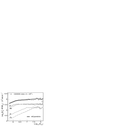
Figure 17: EAS size spectrum with an enlarged shower core selection criterion ($R<50$ m) (symbols), and expected shower spectra for each of the primary nuclei and the mixed composition (lines and shaded areas), with parameters from Table 1 and for the SIBYLL interaction model.

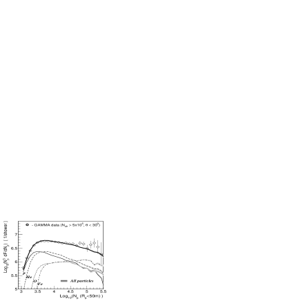
Figure 18: Same as Fig. 16 for the EAS truncated muon size spectra.

A further check of the consistency of the GAMMA facility EAS data with the derived solutions is shown in Figs. 17 and 18, which display the EAS size and truncated muon size spectra (symbols) for an enlarged core selection criterion of $R<50$ m. This is twice as large as the selection radius of the EAS data in Figs. 6–7, and resulted in about four times the number of selected showers. The lines and shaded areas in Figs. 17–18 correspond to the expected (forward folded) EAS spectra with the parameters of primary energy spectra (3) from Table 1 for the SIBYLL interaction model; the corresponding expected shower spectra for each of primary nuclei are also shown.

5 Conclusion

The consistency of the results obtained by the GAMMA experiment (Figs. 6–11,16–17), at least up to $N_{ch}\simeq 10^{7}$, with the corresponding predictions in the framework of the hypothesis of a rigidity-dependent knee in the primary energy spectra and the validity of the SIBYLL or QGSJET interaction models points toward the following conclusions:

• A rigidity-dependent steepening of primary energy spectra in the knee region (expression 3) describes the EAS data of the GAMMA experiment at least up to $N_{ch}\simeq 10^{7}$ with an average accuracy $<10\%$, with particle magnetic rigidities $E_{R}\simeq 2500\pm 200$ TV (SIBYLL) and $E_{R}\simeq 3100-4200$ TV (QGSJET). The corresponding spectral power-law indices are $\gamma_{1}=2.68\pm 0.02$ and $\gamma_{2}=3.10-3.23$ below and above the knee respectively, and the element group scale factors $\Phi_{A}$ are given in Tables 1–3.

• The abundances and energy spectra obtained for primary $p$, $He$, $O$-like and $Fe$-like nuclei depend on the interaction model. The SIBYLL interaction model is preferable in terms of consistency of the extrapolations of the derived primary spectra (Fig. 12) with direct measurements in the energy range of satellite and balloon experiments [37, 38, 39].

• The derived all-particle energy spectra depend only weakly on the interaction model. They are compatible with independent measurements of this spectrum.

• An anomalous behavior of the EAS muon size and density spectra (Fig. 5b, Figs. 11 and 18) and the EAS age parameter (Fig. 10) for EAS size $N_{ch}>10^{7}$ is observed. A similar behavior of the EAS age parameter has previously been observed in [30, 44]. The observed behavior of the muon size and density spectra may be related to the excess of high-multiplicity cosmic muon events detected by the ALEPH and DELPHI experiments [46, 47].

References

- [1] M. Amenomori et al. (Tibet AS Collaboration), Astrophysical Journal 461 (1996) 408.
- [2] M. Aglietta et al. (EAS-TOP Collaboration), Astropart. Phys. 10 (1999) 1.
- [3] M.A.K. Glasmacher et al., Astropart. Phys. 10 (1999) 291.
- [4] T. Antoni et al. (KASCADE Collaboration), Nucl. Instr. Meth. A513 (2003) 490.
- [5] M. Aglietta et al. (EAS-TOP and MACRO Collaborations), Astropart. Phys. 20 (2004) 641 (astro-ph/0305325 v1 (2003)).
- [6] T. Antoni et al., Astropart. Phys. 24 (2005) 1.
- [7] T. Stanev, P.L. Biermann, T.K. Gaisser, Astron. and Astrophys. 274 (1993) 902.
- [8] A.M. Hillas, Journal of Physics G31 (2005) R95.
- [9] B. Peters, Nuovo Cimento (Suppl.) 14 (1959) 436; B. Peters, Proc. ICRC, Vol. 3, Moscow (1959) 157.
- [10] A.M. Hillas, Ann. Rev. Astron. Astrophys. 22 (1984) 425.
- [11] M.A.K. Glasmacher et al., Astropart. Phys. 12 (1999) 1.
- [12] S.V. Ter-Antonyan, L.S. Haroyan, preprint hep-ex/0003006 (2000).
- [13] S.V. Ter-Antonyan and P.L. Biermann, Proc. 27th Intern. Cosmic Ray Conf., Hamburg (2001) HE054, 1051 (astro-ph/0106091).
- [14] M. Aglietta et al. (EAS-TOP Collaboration), Astropart. Phys. 21 (2004) 583.
- [15] S. Ter-Antonyan and P. Biermann, 28th Intern. Cosmic Ray Conf., Tsukuba, HE1 (2003) 235 (astro-ph/0302201).
- [16] J.R. Hörandel, Astropart. Phys. 21 (2004) 241.
- [17] T.V. Danilova, E.A. Danilova, A.B. Erlykin et al., Nucl. Instr. Meth. A323 (1992) 104.
- [18] V.S. Eganov, A.P. Garyaka et al., J. Phys. G:Nucl. Part. Phys. 26 (2000) 1355.
- [19] M.Z. Zazyan, A.P. Garyaka, R.M. Martirosov and J. Procureur, Nucl. Phys. (Proc.Suppl.) B97 (2001) 294.
- [20] A.P. Garyaka, R.M. Martirosov, J. Procureur et al., J. Phys G:Nucl. Part. Phys. 28 (2002) 2317.
- [21] V.S. Eganov, A.P. Garyaka, L.W. Jones et al., Proc. 28th Intern. Cosmic Ray Conf. Tsukuba, HE1.1 (2003) 49.
- [22] R.M. Martirosov et al., Proc. 29th Intern. Cosmic Ray Conf., Pune, 8 (2005), 9.
- [23] R.S. Fletcher, T.K. Gaisser, P. Lipari, T. Stanev, Phys.Rev. D50 (1994) 5710.
- [24] N.N. Kalmykov, S.S. Ostapchenko, Yad. Fiz. 56 (1993) 105 (in Russian).
- [25] S.V. Ter-Antonyan, R.M. Martirosov et al. Preprint astro-ph/0506588 (2005).
- [26] S.V. Ter-Antonyan et al., Proc. 29th Intern. Cosmic Ray Conf., Pune, 6 (2005), 101.
- [27] S.V. Ter-Antonyan et al., Proc. 29th Intern. Cosmic Ray Conf., Pune, 6 (2005), 105.
- [28] V.V. Avakian, S.A. Arzumanian et al., Proc. Questions of Atom Sci. and Tech. 3/20 (1984) 69 (in Russian).
- [29] V.V. Avakian, O.S. Babadjanian et al., Preprint YERPHI-1167(44)-89, Yerevan (1989).
- [30] V.V. Avakian et al., Proc. 24th Intern. Cosmic Ray Conf., Rome 1 (1995) 348.
- [31] S.V. Ter-Antonyan, Preprint YERPHI-1168(45)-89, Yerevan (1989).
- [32] D. Heck, J. Knapp, J.N. Capdevielle, G. Schatz, T. Thouw, Forschungszentrum Karlsruhe Report, FZKA 6019 (1998).
- [33] H. Ulrich et al., Proc. 27th Intern. Cosmic Ray Conf., Hamburg 1 (2001) 97.
- [34] A.M. Hillas at al., Proc. 11th Intern. Cosmic Ray Conf., Budapest, 3 (1970) 533.
- [35] J.N. Stamenov et al., Trudi FIAN, 109 (1979) 132 (in Russion).
- [36] S.V. Ter-Antonyan and R.S. Ter-Antonyan, Forschungszentrum Karlsruhe Report, FZKA 6215 (1998) 61.
- [37] B. Wiebel-Sooth, P.L. Biermann and H. Meyer, Astron. Astrophys. 330 (1998) 389.
- [38] K. Asakimori et al., Astrophysical Journal, 502 (1998), 278.
- [39] M. Hareyama and T. Shibata (RUNJOB Collaboration), Journal of Phys.: Conference Series 47 (2006) 106.
- [40] R. Glasstetter et al. Proc. 26th Intern. Cosmic Ray Conf., Salt Lake City 1 (1999) 222.
- [41] A. Fasso, A. Ferrari, S. Roesler et al., hep-ph/0306267 (http://www.fluka.org).
- [42] I.M. Sobol’, The Monte Carlo Method, M. Nauka (1968) 64 p. (in Russian).
- [43] W.H. Press, S.A. Teukolsky, W.T. Vetterling and B.P. Flannery, Numerical Recipes in C: The Art of Scientific Computing, Cambridge University Press (1992), p. 316. (see also: http://www.library.cornell.edu/nr/bookcpdf/c7-8.pdf).
- [44] S. Miyake, N. Ito et al., Proc. 16th Intern. Cosmic Ray Conf., Kyoto, 13 (1979) 171.
- [45] I. Silin, Preprint YINDR-810, 1961 (Dubna) (CERN Library, preprint P. 810).
- [46] C. Taylor et al., CERN/LEPC 99-5, LEPC/P9 (1999).
- [47] P.Le Coultre, Proc. 29th Intern. Cosmic Ray Conf., Pune, 10 (2005), 137.