The Local Galaxy 8 µm Luminosity Function

Abstract

A Spitzer Space Telescope survey in the NOAO Deep-Wide Field in Boötes provides a complete, 8 µm-selected sample of galaxies to a limiting (Vega) magnitude of 13.5. In the 6.88 deg² field sampled, 79% of the 4867 galaxies have spectroscopic redshifts, allowing an accurate determination of the local ($z<0.3$) galaxy luminosity function. Stellar and dust emission can be separated on the basis of observed galaxy colors. Dust emission (mostly PAH) accounts for 80% of the 8 µm luminosity, stellar photospheres account for 19%, and AGN emission accounts for roughly 1%. A sub-sample of the 8 µm-selected galaxies have blue, early-type colors, but even most of these have significant PAH emission. The luminosity functions for the total 8 µm luminosity and for the dust emission alone are both well fit by Schechter functions. For the 8 µm luminosity function, the characteristic luminosity is $\nu L_{\nu}^{*}(8.0~{}\micron)=1.8\times 10^{10}$ $L_{\sun}$ while for the dust emission alone it is $1.6\times 10^{10}$ $L_{\sun}$. The average 8 µm luminosity density at $z<0.3$ is $3.1\times 10^{7}$ $L_{\sun}$ Mpc^-3, and the average luminosity density from dust alone is $2.5\times 10^{7}$ $L_{\sun}$ Mpc^-3. This luminosity arises predominantly from galaxies with 8 µm luminosities ($\nu L_{\nu}$) between $2\times 10^{9}$ and $2\times 10^{10}$ $L_{\sun}$, i.e., normal galaxies, not LIRGs or ULIRGs.

1 INTRODUCTION

Galaxy emission in the mid-infrared (3µm–10µm) arises from three main mechanisms (e.g. Piovan, Tantalo, & Chiosi, 2006): 1) the Rayleigh-Jeans tail of stellar emission; 2) emission from heated dust in the interstellar medium (ISM, Césarsky et al., 1996; Roelfsema et al., 1996; Verstraete et al., 1996; Vermeij et al., 2002); and 3) a power law component powered by accreting black holes (Moorwood, 1986; Roche et al., 1991; Elvis et al., 1994). The ISM component displays prominent, broad emission features at 3.3, 6.2, 7.7, 8.6, and 11.3 µm (Gillett et al., 1973; Willner et al., 1977; Phillips, Aitken, & Roche, 1984) often attributed to polycyclic aromatic hydrocarbons (PAH, Léger & Puget 1984; Allamandola et al. 1985; Puget & Léger 1989). Elliptical galaxies typically have little or no dust, and therefore their mid-infrared SEDs are expected to be dominated by stellar emission (Lu et al., 2000, 2003; Pahre et al., 2004a, b). Star-forming galaxies, including the extreme Luminous Infrared Galaxies (LIRG, $L_{IR}>10^{11}$ $L_{\sun}$) and Ultra-Luminous Infrared Galaxies (ULIRG, $L_{IR}>10^{12}$ $L_{\sun}$), show the PAH emission features (Lu et al., 2003; Pahre et al., 2004a; Engelbracht et al., 2005; Genzel et al., 1998; Rigopoulou et al., 1999; Armus et al., 2007). Active nuclei can occur in any galaxy type. Galaxy spectral energy distributions (SEDs) are the sum of radiation from all three mechanisms, and because the proportions vary widely, galaxy SEDs in the mid-infrared are very diverse.

Mid-infrared dust emission luminosity is a good indicator of a galaxy’s star formation rate. It is insensitive to dust obscuration, and it can be measured for large samples of galaxies at both $z\approx 0$ and $z\approx 2$. Roche & Aitken (1985, and earlier papers) showed that mid-infrared feature emission is prominent in star forming galaxies, and ISO spectroscopic studies showed that PAH feature strength increases with other measures of star formation rate (SFR — e.g. Vigroux et al., 1999; Elbaz et al., 2002). Förster Schreiber et al. (2004) argued for a quantitative relationship between PAH strength and SFR, and Wu et al. (2005) confirmed a relationship using Spitzer IRAC 8 µm data to measure the PAH emission.

Although PAH strength is a good SFR indicator, it is not perfect. Galaxies with powerful AGN may have very weak or no PAH emission features visible in their SEDs (Moorwood, 1986; Roche et al., 1991; Genzel et al., 1998; Laurent et al., 2000; Egami et al., 2004; Alonso-Herrero et al., 2005). This doesn’t mean active star formation is absent because, for example, intense ultraviolet radiation produced by the accreting black hole may dissociate PAH (Rigopoulou et al., 1999), especially near the nucleus. PAH features are also weak or absent in the SEDs of galaxies with low metallicities (Engelbracht et al., 2005; Rosenberg, Ashby, Salzer, & Huang, 2006; Wu et al., 2006; Madden, Galliano, Jones, & Sauvage, 2006) or low luminosities (Hogg et al., 2005). At an extreme, Houck et al. (2004) found that the SED of the blue compact galaxy SBS 0335$-$052 shows no PAH emission at all. One possible explanation is that the formation and existence of PAH depends on metallicity. Whatever the limitations of PAH emission as an SFR indicator, it is still important to know how much PAH emission there is in the local Universe and what kinds of galaxies that emission comes from. The results should at least give the SFR from typical galaxies, if not from unusual galaxy types. Understanding the local population is an essential step in determining how the SFR has evolved with time.

The Spitzer Space Telescope offers the opportunity to observe large samples of galaxies at 8 µm. At low redshift, Spitzer’s Infrared Array Camera (IRAC, Fazio et al. 2004) can detect the 6.2, 7.7, and 8.6 µm PAH emission features with its 5.8 and 8.0 µm detector arrays, and IRAC’s wide field-of-view ($5^{\prime}\times 5^{\prime}$) and high sensitivity allow IRAC to map large areas of sky efficiently. Maps at 24 µm made with the Multi-band Imaging Photometer (MIPS — Rieke et al., 2004) are an ideal way of selecting large samples of galaxies with PAH emission at $z\sim 2$ (Papovich et al., 2004; Yan et al., 2004; Houck et al., 2005; Papovich et al., 2006; Webb et al., 2006; Caputi et al., 2006), and many authors (eg Houck et al., 2005; Yan et al., 2005; Lutz et al., 2005; Lagache et al., 2004) have used the Infrared Spectrograph (IRS — Houck et al., 2004) to study the PAH emission features in the high-redshift $2\lesssim z\lesssim 3$ population.

This paper focuses on the 7.7 plus 8.6 µm PAH emission features from galaxies at low redshift detected in the IRAC 8.0 µm band. By combining redshifts and IRAC photometry, we obtain an IRAC 8.0 µm-selected local galaxy sample and derive a local PAH luminosity function. The IRAC 8.0 µm-selected galaxy sample is selected at the same rest wavelength as a MIPS 24 µm-selected sample at $z=2$ (e.g., Caputi et al., 2006) or an AKARI 16 µm-selected sample at $z=1$. A comparison between these populations can thus reveal the effects of evolution between $z=2$ and the present. The paper is arranged as follows: §2 describes the IRAC data and the sample selection. §3 discusses K-corrections for the IRAC bands and shows the color-luminosity relations of the sample galaxies. The luminosity function is presented in §4, and §5 summarizes the results. Distances throughout this paper are based on $H_{0}=70$ km s^-1 Mpc^-1, $\Omega_{M}=0.3$, $\Omega_{\Lambda}=0.7$.

2 OBSERVATIONS AND SAMPLE SELECTION

The IRAC data come from the IRAC Shallow Survey (Eisenhardt et al., 2004), which is one of the major IRAC GTO programs. The data cover 8.5 square degrees in the Boötes field of the NOAO Deep-Wide Field Survey (NDWFS Jannuzi & Dey, 1999). Each sky location was observed with three 30 s frames at 3.6, 4.5, 5.8, and 8.0 µm. To create the images in each waveband, the Basic Calibrated Data (BCD) were mosaiced using the Spitzer Science Center software MOPEX (Makovoz & Khan, 2005). An 8 µm catalog was created using SExtractor (Bertin & Arnouts, 1996). The 5$\sigma$ limiting magnitude at 8.0 µm is 14.9 in the Vega system, equivalent to a flux density of 69 $\mu$Jy (Brodwin et al., 2007). The galaxy surface density at this limit is about 10600 galaxies deg^-2 (Fazio et al., 2004b).

Photometry in all four IRAC bands was performed using the SExtractor double-image mode. For each source in the 8 µm catalog, two magnitudes were derived (Brodwin et al., 2007): (1) an aperture magnitude within a 5″ diameter, corrected to total magnitude using the point spread function (PSF) growth curve for point sources, and (2) a SExtractor “auto” magnitude. Figure 1 shows the difference between these two magnitudes as a function of the aperture magnitude. For objects with angular diameters larger than a few arcseconds, the aperture correction does not fully account for flux outside the aperture, and the aperture magnitude therefore underestimates the source flux. For faint point sources and also for extended sources with low surface brightness, SExtractor chooses too small a size for its “auto” aperture, and the auto magnitudes underestimate the flux (e.g., Fig. 5 of Labbé et al., 2005; Brown et al., 2007). In order to account for these biases, we used the brighter of the two magnitude measurements. For the largest galaxies the auto aperture encircles almost all of the flux and therefore gives total magnitude directly, while for faint galaxies, which are nearly pointlike, the aperture magnitude calibrated for point sources likewise lead to a total magnitude. Flux densities for low surface brightness galaxies may still be underestimated, but these are a small fraction of the sample. All magnitudes in this paper are reported in the Vega magnitude system.

In addition to the photometric data, the AGN and Galaxy Evolution Survey (AGES, Kochanek et al. 2006) has measured 15,052 redshifts in the Boötes field with the Hectospec multi-object spectrograph (Fabricant et al., 1998; Roll, Fabricant, & McLeod, 1998; Fabricant et al., 2005) on the MMT. Redshifts have been measured for 92% of galaxies to a magnitude limit of $[8.0]=13.2$ and 65% of galaxies to $[8.0]=13.8$ in a 6.88 deg² sub-field indicated in Figure 2. We limited the sample to this subfield and to $[8.0]<13.5$ (251 $\mu$Jy) to minimize the redshift incompleteness and to $z<0.3$ to minimize uncertainties in the K-corrections. Beyond $z=0.3$, the strongest PAH feature at 7.7 µm shifts out of the IRAC 8.0 µm band. The sample was also limited to $z>0.02$ to avoid statistical noise from small numbers of nearby galaxies. Figure 3 shows the redshift completeness in the final sample. The sample limit corresponds to a limiting 8 µm absolute magnitude of $-27.7$ at $z=0.3$ (neglecting the K-correction).

The 8.0 µm-selected sample includes normal galaxies, AGN, and stars. Figure 4 shows the $[5.8]-[8.0]$ color as a function of $[3.6]-[4.5]$ for all of the objects in the sample. At low redshift, AGN and galaxies with PAH emission both have red IRAC colors, but the two classes can be separated using IRAC color criteria (Lacy et al., 2004; Stern et al., 2005). Galactic stars and elliptical galaxies are mixed together at colors near (0,0); morphology was needed to distinguish between them. This sample is nearby enough that elliptical galaxies are detectably extended in the NDWFS data. The number of objects of each type are listed in Table 1 — 964 objects, 14% of the photometric sample, are identified as AGN. However, only 42 of the 549 AGN with a measured redshift are at $z<0.3$ whereas 2556 out of the 3667 normal galaxies are at $z<0.3$. The AGN fraction at $z<0.3$ is therefore about 1.6% before allowing for incompleteness. Because AGES preferentially observed AGN candidates, the true AGN fraction is likely to be even lower than this. Known AGN were excluded from the sample, but separate results for them are explicitly mentioned in a few places below. As the results show, unknown AGN should have an insignificant effect on the derived luminosity functions.

3 K-CORRECTIONS

K-corrections for the galaxies in this sample are based on a simple two-component model for the SEDs. In this model, the SED for every galaxy is a linear combination of two fixed SEDs: (1) an old “early-type” stellar population, as might be found in an elliptical galaxy or spiral bulge, and (2) a mix of stars and interstellar emission as might be found in a “late-type” spiral galaxy disk. For each of these components, the SED was determined from an average of the observed SEDs for nearby galaxies that have both 2MASS photometry and ISO spectroscopy (Lu et al., 2003). Ellipticals were used to define the early-type SED, and disk galaxies were used to define the late-type SED. The SED for each of these components was normalized at the rest-frame $K$ band. Eleven model SEDs, ranging from a pure early-type template to a pure late-type template, were created. The late/early ratio for these model SEDs is defined as the ratio of the flux densities of the late-type and early-type components in the rest-frame $K$ band. In addition, a twelfth template matching the M82 SED was included to represent galaxies with high star-formation rates. Figure 5 shows the templates from which the model SEDs were constructed. Convolving each model with the IRAC filter functions gave the K-correction for each of the four IRAC bands as a function of redshift. Figure 6 shows the results. For $z<0.3$, the 3.6 and 4.5 µm K-corrections are almost independent of the models, and the 8.0 µm correction is also nearly model-independent unless the galaxy is early-type-dominated. In contrast, the 5.8 µm K-correction is highly variable because it depends critically on the strength of the 6.2 µm PAH feature.

The suite of SED models spans the observed range of galaxy colors with very few outliers and almost none at $z<0.3$. Figure 7 shows the observed $[4.5]-[8.0]$ galaxy colors as a function of redshift. Given the observed color and redshift for each galaxy, the proportion of early- and late-type SED components was determined by interpolation. This proportion defines the rest-frame colors for the galaxy and thus the K-correction for each of the IRAC magnitudes. The few galaxies with $[4.5]-[8.0]$ colors redder than M82 were assigned the M82 K-corrections. AGN (when considered at all) were assigned K-corrections based on a power law SED between 5.8 and 8.0 µm.

4 RESULTS

4.1 Mid-Infrared Colors of the Sample Galaxies

The galaxy sample divides into two populations in a color-magnitude diagram. Figure 7 shows the 8.0 µm absolute magnitude as a function of rest-frame $[4.5]-[8.0]$ color. Galaxies in the red, late-type population ($[4.5]-[8.0]_{\rm rest}>1.1$, cf. Fig. 8) are star-forming systems with prominent 8 µm PAH emission. According to Pahre et al. (2004b), this color corresponds to Sa and later morphological types. The blue, early-type population consists of galaxies with weak or no PAH emission corresponding to S0/a and earlier types (Pahre et al., 2004b). Figure 9 shows a different color-magnitude diagram, this one based on 3.6 µm magnitude, which is a measure of the stellar luminosity. The early-type population generally has higher stellar luminosity than the late-type population, and galaxies fainter than $[3.6]_{\rm abs}=-24$ are uncommon in the early-type population but common in the late-type one. Within the late-type population, the lack of correlation between the rest-frame $[4.5]-[8.0]$ color and $[3.6]_{\rm abs}$ implies that the 3.6 µm luminosity is little affected by the 3.3 µm PAH emission feature. In contrast, $[8.0]_{\rm abs}$ is strongly correlated with the rest-frame $[3.6]-[4.5]$ color (Fig. 10), especially for $[8.0]_{\rm abs}<-27$. This correlation suggests that dust emission at 4.5 µm is detectable in the star-forming late-type population, i.e., galaxies with strong PAH emission also show dust continuum emission at 4.5 µm. This is consistent with ISOPHOT spectroscopy: Lu et al. (2003) detected 4 µm dust emission from nearby spiral galaxies and suggested it arises from a dust component closely related to the PAH. The same UV sources that heat PAH molecules may also heat the dust that produces the excess 4.5 µm emission. Dust emission at 4.5 µm is relatively unimportant for the least luminous galaxies, those with $[8.0]_{\rm abs}>-26$, despite the presence of 8 µm emission in a subset of the low-luminosity galaxies (Fig. 7).

The 8 µm number counts are strongly dominated by the late-type population: only 3% of the spectroscopic sample have early-type colors. Even for the early-type-dominated galaxies, most of the 8 µm emission comes from dust rather than stellar light (Fig. 8). The late-type galaxies are even more dominant in 8 µm luminosity, as shown in Fig. 7. All the early-type galaxies have 8 µm absolute magnitudes at least three magnitudes fainter than the brightest late-type galaxies.

4.2 The 8.0 µm Luminosity Function

There are many ways to estimate the galaxy luminosity function from survey data. When examining a new wavelength regime, a non-parametric method — one not assuming a specific functional form — is desirable because the true luminosity function may not follow a Schechter or other typical distribution. For the present survey, where galaxy distances vary by a factor of ten, it is also better to avoid methods that are sensitive to possible galaxy clustering. Willmer (1997) and Takeuchi, Yoshikawa, & Ishii (2000) have presented detailed comparisons of many methods. We have computed the luminosity functions with both the familiar $1/V_{\rm max}$ method (Schmidt, 1968) and the Lynden-Bell (1971) C^- method. The C^- method does not require binning the data, thus avoiding the possible bias in $1/V_{\rm max}$ found by Page & Carrera (2000), and it is insensitive to possible galaxy clustering. The results of the two methods are consistent. A further verification that large scale structure has little effect was to ignore data in narrow but heavily populated redshift ranges such as $z\approx 0.13$ and $z\approx 0.19$ (Fig. 8). The resulting luminosity functions do not change significantly.

The luminosity functions have to be corrected for spectroscopic incompleteness in the sample. Because this sample has spectra for nearly all galaxies (Table 1, Fig. 3), the incompleteness correction has an insignificant effect on the results except in the faintest luminosity bins. This was checked by recomputing the luminosity function with two different incompleteness corrections. One method was to use only galaxies with spectroscopic redshifts but apply a weight to each one according to the reciprocal probability it would have been observed in the spectroscopic sample. The second method included all galaxies. Galaxies were divided into bins based on $[4.5]-[8.0]$ colors and $[8.0]$ magnitudes, and galaxies without redshifts were assigned the same redshift distribution as the galaxies with known redshifts in the same bin. The two methods give luminosity functions that are equal within the Poisson uncertainties.

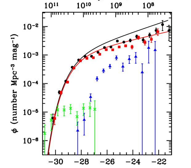
Figure 11: Derived differential luminosity functions corrected for spectroscopic incompleteness. Black dots denote the 8 µm luminosity function for all galaxies excluding AGN, and red squares denote the luminosity function for PAH alone, i.e., after subtracting the stellar continuum emission for each galaxy. These two luminosity functions were derived from the non-parametric C^- method. Blue triangles denote the luminosity function for early-type galaxies, specifically those with $[4.5]-[8.0]<1.1$. Even for these galaxies, much of the emission is PAH despite the color selection. Green crosses denote the luminosity function for AGN. These latter two luminosity functions were derived from the $1/V_{max}$ method because of the smaller numbers of galaxies. Because of the small numbers, the blue galaxy luminosity function is only reliable for $-27\lesssim[8.0]_{abs}\lesssim-25$. The AGN luminosity function is highly uncertain throughout; only one bin has as many as 8 galaxies in it. All points are slightly offset horizontally for clarity; see Tables 2 and 3 for actual magnitude bins. Error bars show the Poisson uncertainties in each bin. Lines show the respective parametric Schechter functions that best fit the data for “all 8 µm emission” and “PAH only.” Both were derived from the STY method. The bottom axis is labeled in 8 µm Vega magnitudes, while the top axis is labeled in the equivalent $\nu L_{\nu}$ units.

The non-parametric 8.0 µm luminosity functions for various galaxy classes are shown in Figure 11 and Tables 2 and 3. As shown in this figure and also Figure 7, blue galaxies contribute little to the luminosity function and are rare for $[8.0]_{\rm abs}<-26$. AGN are insignificant except in the brightest luminosity bins, where the uncertainties are large because few objects are in the survey. The luminosity function in the range $-29.5\lesssim[8.0]_{\rm abs}\lesssim-22$ is dominated by galaxies with significant dust contribution to the 8 µm flux.

In addition to total luminosity, the observations allow us to measure the 8.0 µm PAH (dust) luminosity alone. For each galaxy in the sample, the rest-frame 3.6 µm flux density was scaled by a factor of 0.227 (an estimate of the stellar flux density at 8 µm — Pahre et al., 2004a) and subtracted from the rest-frame 8.0 µm flux density. This subtracts the starlight, leaving the PAH flux density. Because the subtraction is done on rest-frame flux densities, the procedure is equivalent to the two-component decomposition illustrated in Fig. 8. After subtracting the continuum, galaxies with residual 8.0 µm magnitudes fainter than the limiting magnitude $[8.0]=13.5$ were excluded from the sample, and the luminosity function was re-calculated for the remaining galaxies to give a PAH-only luminosity function. The result is shown in Figure 11 and Tables 2 and 3.

The uncertainties in the luminosity functions are set both by Poisson statistics of the sample and by cosmic variance. The Poisson uncertainties for the $1/V_{\rm max}$ method are given in Table 2 and statistical uncertainties for the $C^{-}$ method in Table 3. Cosmic variance uncertainty can be estimated (Davis & Huchra, 1982) from the volume sampled plus an estimate of the galaxy two-point correlation function. This is not known directly for the 8 µm sample, but we assume it’s the same as for optically-selected galaxy samples. (If anything, the correlation function is likely to be smaller for 8 µm-selected galaxies, which are predominantly late-type, than for optically-selected ones, more of which are early-type — Norberg et al. 2002. This will lead to less cosmic variance for an 8 µm-selected sample.) In practice, a correlation function based on the fluctuation power spectrum from WMAP-1 (Spergel et al., 2003) was extrapolated to the present via the method of Seljak & Zaldarriaga (1996) then transformed via a spherical Bessel function and smoothed with a 1 Mpc radius. The volume integral (e.g., Newman & Davis, 2002, Eq. 1) was then evaluated via a Monte Carlo approach. The resulting cosmic variance uncertainty is $\approx$15% in bins $[8.0]_{\rm abs}<-27.7$, where the survey samples the full volume of $z\leq 0.3$. This is a single uncertainty for the entire luminosity function, not an independent uncertainty in each bin. In the fainter bins, the uncertainty should in principle be larger, but the entire method is based on the assumption that the luminosity function is constant within the volume surveyed. In the faintest bin, for example, the survey magnitude limit corresponds to 135 Mpc, and the data give no information whatsoever on the luminosity function outside this distance. Density peaks in the sample are evident in Figure 8 but do not affect the derived luminosity function.

As it turns out, a Schechter function is an excellent fit to both the total 8.0 µm and the PAH luminosity functions, as shown in Figure 11. Table 4 gives the best-fit parameters as found using the STY maximum likelihood method (Sandage, Tammann, & Yahil, 1979), and Figure 12 shows the interdependence of the derived characteristic magnitudes $M^{*}$ and faint-end slopes $\alpha$. The derived Schechter exponents for the middle to faint end slopes are $\alpha=-1.38$ and $\alpha=-1.26$ respectively. The slopes are similar to those found in the Sloan $r$ band (Loveday, 2004; Xia et al., 2006) and the infrared $K$ band (Huang, Glazebrook, Cowie, & Tinney, 2003; Jones, Peterson, Colless, & Saunders, 2006) over a similar redshift range, though Blanton et al. (2003) found a slightly shallower slope in $r$. The steeper slope for the total luminosity shows that fainter galaxies tend to have relative less PAH emission compared to their stellar emission (though the slope uncertainties overlap at the 2$\sigma$ level, as seen in Fig. 12 and Table 4). The inactive “blue” galaxies have just as steep a faint-end slope ($\alpha=-1.39$) as the entire sample, in contrast to the result in blue light, where inactive galaxies show a much shallower faint-end slope (Madgwick, Hewett, Mortlock, & Lahav, 2002). At the bright end, $L>L^{*}$, there are no excess galaxy numbers above the Schechter function prediction, in contrast to the results of Saunders et al. (1990) for the IRAS 60 µm luminosity function. The high luminosity population, i.e., LIRGs and ULIRGs, consists of galaxies with far-infrared color temperatures $>$36 K (Saunders et al., 1990), characteristic of Seyfert and starburst galaxies. Our exclusion of AGN in the 8.0 µm sample, which removed galaxies from the bright end of the luminosity function, does not explain why a Schechter function can fit the remainder of the sample.

Integrating the luminosity functions over the whole sample gives the total 8 µm luminosity density in the local Universe. The result is $3.1\times 10^{7}~{}$$L_{\sun}$ Mpc^-3 for total 8 µm luminosity density (not including AGN), $2.5\times 10^{7}~{}\mbox{$L_{\sun}$}$ Mpc^-3 for PAH luminosity density, and a highly uncertain $0.05\times 10^{7}~{}\mbox{$L_{\sun}$}$ Mpc^-3 for AGN luminosity density. (The sample is too small to determine reliable AGN numbers.) Thus over the entire galaxy population, stellar emission contributes about 19% of the 8.0 µm luminosity while dust emission contributes 80% and AGN roughly 1%. Galaxies with $2\times 10^{9}~{}\mbox{$L_{\sun}$}<\nu L_{\nu}(8.0\micron)<2\times 10^{10}$ $L_{\sun}$ contribute 50% of the total 8 µm luminosity, and galaxies above and below this range contribute about 25% each. Thus the dominant contribution to the PAH luminosity density comes from normal galaxies, not LIRGs or ULIRGs.

4.3 Star Formation Rates

Star formation rates in the local universe have been measured by a variety of techniques. (See the review by Kennicutt 1998a.) Hopkins (2004) compiled star formation rate densities (SFRD) from a variety of tracers. According to Hopkins’ compilation, over the $z<0.3$ range of the present survey, the volume-weighted average ${\rm SFRD}\approx 0.031$ $M_{\sun}$ yr^-1 Mpc^-3, though some tracers tend to be systematically higher (emission lines) or lower (ultraviolet) than this value. Martin et al. (2005) combined ultraviolet with far infrared data and found a local ($z<0.04$) ${\rm SFRD}\approx 0.021$ $M_{\sun}$ yr^-1 Mpc^-3, about 20% higher than but consistent with Hopkins’ result at this much smaller redshift.

Dust emission at 8.0 µm is correlated with the total infrared luminosity $L_{IR}$ in galaxies (Rigopoulou et al., 1999; Elbaz et al., 2002; Lu et al., 2003) although the relation is non-linear (Lu et al., 2003) and has large scatter (e.g., Fig. 17 of Smith et al., 2007). In normal star-forming galaxies, the integrated flux between 5.8 and 11.3 µm is between 9% (for galaxies Lu et al. call “FIR-quiescent”) and 5% (for Lu et al. “FIR-active” galaxies) of $L_{IR}$ (Lu et al., 2003). Recent results from Spitzer are consistent with these values; Smith et al. (2007) find that in the central areas of normal galaxies, the 7.7 µm PAH complex can contribute up to 10% of $L_{IR}$. In ULIRGs, PAH emission in the 5.8–11.3 µm range is lower at $\lesssim$1% of $L_{IR}$ (Rigopoulou et al., 1999; Armus et al., 2007); this could be partly due to an AGN contributing to $L_{IR}$. Despite the uncertainties, some authors (e.g., Förster Schreiber et al., 2004; Wu et al., 2005) have suggested that $\nu L_{\nu}({\rm PAH})$ can be used to measure star formation rates for galaxies, and Wu et al. (2005) derived ${\rm SFR}\approx\nu L_{\nu}({\rm PAH})/(1.5\times 10^{9}~{}\mbox{$L_{\sun}$})$ $M_{\sun}$ yr^-1. This result was based on a sample of Sloan galaxies showing H$\alpha$ emission. The PAH luminosity density found in §4.2 combined with the local SFRD (Hopkins, 2004, Fig. 2) integrated from $z=0$ to 0.3 gives a volume average ${\rm SFR}\approx\nu L_{\nu}({\rm PAH})/(0.84\times 10^{9}~{}\mbox{$L_{\sun}$})$ $M_{\sun}$ yr^-1, about double that found by Wu et al. for individual galaxies. In other words, the volume-averaged PAH luminosity density is half as much as expected, given the volume-averaged SFRD and ${\rm SFRD}/\nu L_{\nu}({\rm PAH})$ ratios of individual galaxies. The difference suggests that the galaxy samples have been weighted to galaxies with unusually large PAH emission for their SFRs, but this is hard to understand if the dominant contribution to star formation comes from the normal galaxy population (e.g., Le Floc’h et al., 2005).

5 SUMMARY

An 8.0 µm-selected sample of low redshift ($z<0.3$) galaxies finds primarily star-forming galaxies. AGN represent less than 2% of the sample both by number and by fraction of the 8 µm luminosity. The luminosity function of the remaining galaxies can be described as a Schechter function with characteristic magnitude $M^{*}=-28.46$ (corresponding to $\nu L_{\nu}=1.8\times 10^{10}$ $L_{\sun}$) and $\alpha=-1.38$. Subtracting starlight continuum emission from each galaxy gives a luminosity function for emission from the interstellar medium component (mostly PAH) alone. This can also be approximated by a Schechter function with characteristic magnitude $M^{*}=-28.34$ ($\nu L_{\nu}=1.6\times 10^{10}$ $L_{\sun}$) and $\alpha=-1.26$.

The total 8.0 µm luminosity density for this 8.0 µm-selected sample is $3.1\times 10^{7}$ $L_{\sun}$ Mpc^-3. Ignoring the luminosity contributed by AGN, about 81% of the 8 µm luminosity is from interstellar dust emission, presumably PAH, and about 19% is from stellar photospheres. The observed, volume-averaged ratio of PAH luminosity density to star formation rate density is about half of an estimate based on local, individual galaxies.

Figure 1: Difference between the SExtracter total (“auto”) magnitudes and 5″ aperture magnitudes. Offsets are mostly positive, indicating that aperture magnitudes underestimate the total flux of resolved galaxies. We selected the sample using the aperture magnitudes to avoid bias against lower surface brightness galaxies, and set the magnitude limit at $[8.0]=13.5$. The derived luminosity functions are based on the auto magnitudes for the resolved galaxies and the aperture magnitudes for the unresolved galaxies.

Figure 2: The Böotes field showing the approximate area of 8 µm coverage outlined in red. Positions are J2000. Black dots denote denote the 8.0 µm-detected galaxies that have AGES spectroscopic redshifts. The black lines enclose the area of the highly complete redshift sample used for this paper.

Figure 3: Redshift identification fraction in each half-magnitude bin (filled circles, left ordinate label). Error bars show the Poisson uncertainty. The solid line shows the histogram of the 8 µm magnitude distribution of all galaxies in the catalog (right ordinate label). Only galaxies with $[8.0]<13.5$ are in the final sample.

Figure 4: $[5.8]-[8.0]$ vs $[3.6]-[4.5]$ color-color diagram for separation of AGN, star-forming galaxies, and early type galaxies (Stern et al., 2005). Data are plotted as observed, i.e., before K-correction. Black dots denote normal galaxies, red dots denote stars, and blue dots denote AGN, all as classified by optical spectroscopy. The two thick lines show two SED models from $0<z<0.6$, one with and the other without PAH emission. (The latter is almost hidden behind the data near zero color.) The thin solid lines show the Stern et al. (2005) AGN-galaxy separation criterion; AGN lie within the quadrilateral extending to the top of the plot. The color cut at $[5.8]-[8.0]=0.5$ separates stars and elliptical galaxies from galaxies with significant PAH emission. Galaxies with PAH emission cannot enter the “no PAH” area unless their redshifts are $>$0.6.

Figure 5: Galaxy SED templates. The upper curve shows the M82 template, the middle curve the spiral (“late-type”) template, and the bottom curve the elliptical (“early-type”) template. The vertical axis is in arbitrary units. The early-type template is an average ISOPHOT-S spectrum of six classical elliptical galaxies compiled by Lu et al. (2000). It is very similar to the elliptical spectrum shown by Lu et al. (2003) except at wavelengths longer than 8 µm, where an improved ISOPHOT-S calibration made the current spectrum slightly steeper (i.e., bluer). The late-type template is the average for spiral galaxies from Lu et al. (2000). Nine additional templates used in this paper are mixtures of the early- and late-type templates.

Figure 6: K-corrections for the four IRAC channels for each of the twelve SED models. The bottom line in each panel shows the early-type model. The 3.6 and 4.5 µm bands sample mainly stellar emission longward of the Wien peak and therefore show a negative K-correction. The 5.8 µm band is relatively narrow and shows a positive K-correction, depending on the amount of PAH present, as the 6.2 µm PAH feature leaves the band at $z\approx 0.05$. As redshift increases further, the band samples only stellar emission, and the K-correction decreases. The 8 µm band is wide, and the 7.7 µm feature remains inside the band at low redshift. As redshift increases, the 6.2 µm PAH feature enters the band before the 7.7 µm feature leaves, leading to a nearly constant K-correction. At $z\gtrsim 0.2$, the 7.7 µm feature begins to leave the band, and the K-correction increases according to the PAH strength.

Figure 7: Color-magnitude diagram showing $[4.5]-[8.0]$ color versus 8 µm absolute magnitudes. Points denote galaxies with spectroscopic redshifts. Colors and magnitudes are both corrected to the rest frame. Most galaxies show strong PAH emission ($[4.5]-[8.0]>2$) and are therefore in the “late-type” category as we have defined it. “Early-type” galaxies with weak or no PAH emission ($[4.5]-[8.0]\lesssim 0.4$) are well separated in this diagram from the much larger late-type population, but galaxies span the entire color range. None of the early-type galaxies has high luminosity at 8 µm.

Figure 8: The $[4.5]-[8.0]$ color versus redshift for galaxies with spectroscopic redshifts. Points denote the observed galaxies with AGN excluded. Lines show colors for each of twelve model SEDs as a function of redshift. The reddest model is derived from the M 82 SED. Other models are a linear combination of late-type and early-type templates as shown in Fig. 5. These SEDs are normalized at rest 2.2 µm with the stellar fraction going from 0 to 1 in steps of 0.1 from the bluest model to the reddest one (second-reddest including the M82 model). Only galaxies with $z<0.3$ are used in this paper.

Figure 9: Color-magnitude diagram showing $[4.5]-[8.0]$ color vs 3.6 µm absolute magnitudes. Points denote galaxies with spectroscopic redshifts. Colors and magnitudes are both corrected to the rest frame. The upper luminosity envelope is populated by both blue ($[4.5]-[8.0]<1.1$) and star-forming galaxies, but there are no blue galaxies with low 3.6 µm luminosities. For the strongly star-forming galaxies, $[4.5]-[8.0]\gtrsim 2$, color does not correlate with the absolute 3.6 µm magnitude.

Figure 10: Color-magnitude diagram showing $[3.6]-[4.5]$ color vs 8 µm absolute magnitudes. Points denote galaxies with spectroscopic redshifts. Colors and magnitudes are both corrected to the rest frame. The correlation between color and magnitude indicates that dust emission may constitute about 30% of the total 4.5µm emission for galaxies with $[8.0]_{\rm abs}\lesssim-27$.

Figure 12: Uncertainty ellipses for characteristic magnitude $M^{*}$ and faint end slope $\alpha$ of the Schechter luminosity functions. The ellipses were calculated using a grid in $M^{*}$–$\alpha$ space and the STY formalism. The curves represent contours of constant $\Delta\chi^{2}$ corresponding to 1$\sigma$ (inner), 2$\sigma$ (middle), and 3$\sigma$ (outer) confidence levels assuming three fitting parameters. Statistical uncertainty in the overall normalization $\Phi^{*}$ is very small, but the true uncertainty is set by cosmic variance (§4.2). Faint end slopes probably differ but are consistent at the 2$\sigma$ level.

Table 1

Number of Objects at $[8.0]<13.5$

Object	Total	Redshift Sample	$z<0.3$
Star	1894	0	0
Blue Galaxies	236	109	100
Star-Forming Galaxies	3667	3174	2556
AGN	964	549	42

Table 2

Luminosity Functions Calculated by the $1/V_{max}$ Method

[8.0]abs	$\nu L_{\nu}(8~{}\micron)$	$N$	$\phi$(8.0µm)	$\Delta\phi$(8.0µm)	$N$	$\phi$(PAH)	$\Delta\phi$(PAH)
			$10^{-3}$ Mpc-3 mag-1			$10^{-3}$ Mpc-3 mag-1
-30.27	$9.5\times 10^{10}$	2	00.003	00.002	2	00.003	00.002
-29.77	$6.0\times 10^{10}$	10	00.018	00.006	9	00.016	00.005
-29.27	$3.8\times 10^{10}$	37	00.073	00.012	31	00.062	00.011
-28.77	$2.4\times 10^{10}$	133	0.25	0.02	116	0.22	0.02
-28.27	$1.5\times 10^{10}$	294	0.56	0.03	268	0.50	0.03
-27.77	$9.5\times 10^{9\phantom{0}}$	447	1.06	0.05	384	0.86	0.04
-27.27	$6.0\times 10^{9\phantom{0}}$	429	1.45	0.07	416	1.34	0.07
-26.77	$3.8\times 10^{9\phantom{0}}$	413	2.07	0.10	367	1.75	0.09
-26.27	$2.4\times 10^{9\phantom{0}}$	327	2.49	0.14	270	1.94	0.12
-25.77	$1.5\times 10^{9\phantom{0}}$	218	2.71	0.18	179	2.04	0.15
-25.27	$9.5\times 10^{8\phantom{0}}$	137	3.20	0.30	98	2.02	0.20
-24.77	$6.0\times 10^{8\phantom{0}}$	63	2.50	0.30	64	2.17	0.27
-24.27	$3.8\times 10^{8\phantom{0}}$	41	3.00	0.50	27	1.73	0.33
-23.77	$2.4\times 10^{8\phantom{0}}$	23	3.70	0.80	13	1.60	0.44
-23.27	$1.5\times 10^{8\phantom{0}}$	9	2.40	0.80	16	3.00	0.80
-22.77	$9.5\times 10^{7\phantom{0}}$	12	7.40	2.10	7	3.20	1.20
-22.27	$6.0\times 10^{7\phantom{0}}$	7	7.70	2.90	6	5.80	2.40
-21.77	$3.8\times 10^{7\phantom{0}}$	1	2.40	2.40	$\cdots$	$\cdots$	$\cdots$
-21.27	$2.4\times 10^{7\phantom{0}}$	2	10.100	7.60	$\cdots$	$\cdots$	$\cdots$

Table 3

Luminosity Functions Calculated by the C^- Method

[8.0]abs	$\nu L_{\nu}(8~{}\micron)$	$\phi$(8.0µm)	$\Delta\phi$(8.0µm)	$\phi$(PAH)	$\Delta\phi$(PAH)
		$10^{-3}$ Mpc-3 mag-1		$10^{-3}$ Mpc-3 mag-1
-30.13	$8.5\times 10^{10}$	00.006	00.002	00.006	00.002
-29.63	$5.3\times 10^{10}$	00.049	00.007	00.048	00.007
-29.13	$3.4\times 10^{10}$	00.121	00.010	00.112	00.009
-28.63	$2.1\times 10^{10}$	0.37	0.02	0.35	0.02
-28.13	$1.5\times 10^{10}$	0.67	0.02	0.63	0.02
-27.63	$8.5\times 10^{9\phantom{0}}$	0.89	0.02	0.76	0.02
-27.13	$5.3\times 10^{9\phantom{0}}$	0.90	0.02	0.80	0.02
-26.63	$3.4\times 10^{9\phantom{0}}$	1.24	0.03	1.06	0.03
-26.13	$2.1\times 10^{9\phantom{0}}$	1.82	0.06	1.54	0.05
-25.63	$1.5\times 10^{9\phantom{0}}$	1.92	0.08	1.53	0.07
-25.13	$8.5\times 10^{8\phantom{0}}$	3.10	0.20	1.92	0.12
-24.63	$5.3\times 10^{8\phantom{0}}$	2.80	0.20	2.10	0.17
-24.13	$3.4\times 10^{8\phantom{0}}$	3.30	0.40	1.91	0.27
-23.63	$2.1\times 10^{8\phantom{0}}$	4.50	0.60	4.10	0.50
-23.13	$1.5\times 10^{8\phantom{0}}$	3.40	0.60	2.80	0.50
-22.63	$8.5\times 10^{7\phantom{0}}$	5.00	0.90	3.60	0.80
-22.13	$5.3\times 10^{7\phantom{0}}$	7.30	1.50	6.60	1.70
-21.63	$3.4\times 10^{7\phantom{0}}$	11.700	4.50	$\cdots$	$\cdots$
-21.13	$2.1\times 10^{7\phantom{0}}$	7.20	3.90	$\cdots$	$\cdots$

Table 4

Schechter Function Parameters

	all 8 µm emission	PAH only
$M^{*}(8~{}\micron)$	$-28.46\pm 0.08$	$-28.34\pm{0.08}$
$L^{*}(8~{}\micron)$	$1.8\times 10^{10}$	$1.6\times 10^{10}$ $L_{\sun}$
$\Phi^{*}$	$1.10\times 10^{-3}$	$1.17\times 10^{-3}$
$\alpha$	$-1.38\pm 0.04$	$-1.26\pm 0.04$
Integrated luminosity	$3.1\times 10^{7}$	$2.5\times 10^{7}$ $L_{\sun}$ Mpc-3

References

- Allamandola et al. (1985) Allamandola, L. J., Tielens, A. G. G. M., & Barker, J. R. 1985, ApJ, 290, L25
- Allamandola et al. (1989) Allamandola, L. J., Tielens, A. G. G. M., & Barker, J. R. 1989, ApJS, 71, 733
- Alonso-Herrero et al. (2004) Alonso-Herrero, A., et al. 2004, ApJS, 154, 155
- Alonso-Herrero et al. (2005) Alonso-Herrero, A., et al. 2006, ApJ, 640, 167
- Armus et al. (2007) Armus, L., et al. 2007, ApJ, 656, 148
- Bell (2003) Bell, E. F. 2003, ApJ, 586, 794
- Bertin & Arnouts (1996) Bertin, E. & Arnouts, S. 1996, A&A,117,393
- Blanton et al. (2003) Blanton, M. R., et al. 2003, ApJ, 592, 819
- Brodwin et al. (2007) Brodwin, M., et al. 2007, ApJ, submitted
- Brown et al. (2007) Brown, M. J. I., Dey, A., Jannuzi, B. T., Brand, K., Benson, A. J., Brodwin, M., Croton, D. J., & Eisenhardt, P. R. 2007, ApJ, 654, 858
- Caputi et al. (2006) Caputi, K. I., et al. 2006, ApJ, 637, 727
- Césarsky et al. (1996) Césarsky, D., Lequeux, J., Abergel, A., Perault, M., Palazzi, E., Madden, S., & Tran, D. 1996, A&A, 315, L309
- Crawford, Marr, Partridge, & Strauss (1996) Crawford, T., Marr, J., Partridge, B., & Strauss, M. A. 1996, ApJ, 460, 225
- Dale et al. (2003) Dale, D., et al. 2003, AJ, 120, 583
- Davis & Huchra (1982) Davis, M. & Huchra, J. 1982, ApJ, 254, 437.
- Egami et al. (2004) Egami, E., et al. 2004, ApJS, 154, 130
- Eisenhardt et al. (2004) Eisenhardt, P., et al. 2004, ApJS, 154, 48
- Elbaz et al. (2002) Elbaz, D., Cesarsky, C. J., Chanial, P., Aussel, H., Franceschini, A., Fadda, D., & Chary, R. R. 2002, A&A, 384, 848
- Elvis et al. (1994) Elvis, M., et al. 1994, ApJS, 95, 1
- Engelbracht et al. (2005) Engelbracht, C. W., et al. 2005, ApJ, 628, L29
- Fabricant et al. (1998) Fabricant, D. G., Hertz, E. N., Szentgyorgyi, A. H., Fata, R. G., Roll, J. B., & Zajac, J. M. 1998, Proc. SPIE, 3355, 285
- Fabricant et al. (2005) Fabricant, D., et al. 2005, PASP, 117, 1411
- Fazio et al. (2004a) Fazio, G. G., et al. 2004, ApJS, 154, 10
- Fazio et al. (2004b) Fazio, G. G., et al. 2004, ApJS, 154, 39
- Flores et al. (1999) Flores, H., et al. 1999, ApJ, 517, 148
- Förster Schreiber et al. (2004) Förster Schreiber, N. M., et al. 2004, ApJ, 616, 40
- Genzel et al. (1998) Genzel, R., et al. 1998, ApJ, 498, 579
- Gillett et al. (1973) Gillett, F. C., Forrest, W. J., & Merrill, K. 1973, ApJ, 183, 87
- Haarsma et al. (2000) Haarsma, D. B., Partridge, R. B., Windhorst, R. A., & Richards, E. A. 2000, ApJ, 544, 641
- Hammer et al. (1997) Hammer, F., et al. 1997, ApJ, 481, 49
- Hogg et al. (1998) Hogg, D. W., Cohen, J. G., Blandford, R., & Pahre, M. A. 1998, ApJ, 504, 622
- Hogg et al. (2005) Hogg, D., et al. 2005, ApJ, 624, 162
- Hopkins (2004) Hopkins, A. M. 2004, ApJ, 615, 209
- Houck et al. (2004) Houck, J. R., et al. 2004, ApJS, 154, 211
- Houck et al. (2005) Houck, J. R., et al. 2005, ApJ, 622, L105
- Huang, Glazebrook, Cowie, & Tinney (2003) Huang, J.-S., Glazebrook, K., Cowie, L. L., & Tinney, C. 2003, ApJ, 584, 203
- Jannuzi & Dey (1999) Jannuzi, B. T., & Dey, A. 1999, ASP Conf. Ser. 191: Photometric Redshifts and the Detection of High Redshift Galaxies, 191, 111
- Jones, Peterson, Colless, & Saunders (2006) Jones, D. H., Peterson, B. A., Colless, M., & Saunders, W. 2006, MNRAS, 369, 25
- Kennicutt (1998a) Kennicutt, R. C., Jr. 1998, ARA&A, 36, 189
- Kennicutt (1998b) Kennicutt, R. C. 1998, ApJ, 498, 541
- Kochanek et al. (2006) Kochanek, C., et al. 2007, in preparation
- Labbé et al. (2005) Labbé, I., et al. 2005, ApJ, 624, L81
- Lacy et al. (2004) Lacy, M., et al. 2004, ApJS, 154, 166
- Lagache et al. (2004) Lagache, G., et al. 2004, ApJS, 154, 112
- Laurent et al. (2000) Laurent, O., Mirabel, I. F., Charmandaris, V., Gallais, P., Madden, S. C., Sauvage, M., Vigroux, L., & Cesarsky, C. 2000, A&A, 359, 887
- Le Floc’h et al. (2005) Le Floc’h, E., et al. 2005, ApJ, 632, 169
- Léger & Puget (1984) Léger, A., & Puget, J. L. 1984, A&A, 137, L5
- Lilly et al. (1996) Lilly, S. J., Le Fevre, O., Hammer, F., & Crampton, D. 1996, ApJ, 460, L1
- Loveday (2004) Loveday, J. 2004, MNRAS, 347, 601.
- Lu et al. (2000) Lu, N., & Hur, M. 2000, BAAS, 196, 2702
- Lu et al. (2003) Lu, N., et al. 2003, ApJ, 588, 199
- Lutz et al. (2005) Lutz, D., Valiante, E., Sturm, E., Genzel, R., Tacconi, L. J., Lehnert, M. D., Sternberg, A., & Baker, A. J. 2005, ApJ, 625, L83
- Lynden-Bell (1971) Lynden-Bell, D. 1971, MNRAS, 155, 95
- Madden, Galliano, Jones, & Sauvage (2006) Madden, S. C., Galliano, F., Jones, A. P., & Sauvage, M. 2006, A&A, 446, 877
- Madgwick, Hewett, Mortlock, & Lahav (2002) Madgwick, D. S., Hewett, P. C., Mortlock, D. J., & Lahav, O. 2002, MNRAS, 334, 209
- Makovoz & Khan (2005) Makovoz, D., & Khan, I. 2005, ASP Conf. Ser. 347: Astronomical Data Analysis Software and Systems XIV, 347, 81
- Martin et al. (2005) Martin, D. C., et al. 2005, ApJ, 619, L59
- Moorwood (1986) Moorwood, A. FṀ1̇986, A&A, 166, 4
- Newman & Davis (2002) Newman, J. A. & Davis, M. 2002, ApJ, 564, 567
- Norberg et al. (2002) Norberg, P., et al. 2002, MNRAS, 332, 827
- Page & Carrera (2000) Page, M. J. & Carrera, F. J. 2000, MNRAS, 311, 433
- Pahre et al. (2004a) Pahre, M. A., Ashby, M. L. N., Fazio, G. G., & Willner, S. P. 2004, ApJS, 154, 229
- Pahre et al. (2004b) Pahre, M. A., Ashby, M. L. N., Fazio, G. G., & Willner, S. P. 2004, ApJS, 154, 235
- Papovich et al. (2004) Papovich, C., et al. 2004, ApJS, 154, 70
- Papovich et al. (2006) Papovich, C., et al. 2006, ApJ, 640, 92
- Phillips, Aitken, & Roche (1984) Phillips, M. M., Aitken, D. K., & Roche, P. F. 1984, MNRAS, 207, 25
- Piovan, Tantalo, & Chiosi (2006) Piovan, L., Tantalo, R., & Chiosi, C. 2006, MNRAS, 366, 923
- Puget & Léger (1989) Puget, J. L. & Léger, A. 1989, ARA&A, 27, 161
- Rieke et al. (2004) Rieke, G. H., et al. 2004, ApJS, 154, 25
- Rigopoulou et al. (1999) Rigopoulou, D., Spoon, H. W. W., Genzel, R., Lutz, D., Moorwood, A. F. M., & Tran, Q. D. 1999, AJ, 118, 2625
- Roelfsema et al. (1996) Roelfsema, P. R., et al. 1996, A&A, 315, L289
- Roche & Aitken (1985) Roche, P. F., & Aitken, D. K. 1985, MNRAS, 213, 789
- Roche et al. (1991) Roche, P. F., Aitken, D. K., Smith, C. H., & Ward, M. J. 1991, MNRAS, 248, 606
- Roll, Fabricant, & McLeod (1998) Roll, J. B., Fabricant, D. G., & McLeod, B. A. 1998, Proc. SPIE, 3355, 324
- Rosenberg, Ashby, Salzer, & Huang (2006) Rosenberg, J. L., Ashby, M. L. N., Salzer, J. J., & Huang, J.-S. 2006, ApJ, 636, 742
- Rush, Malkan, & Spinoglio (1993) Rush, B., Malkan, M. A., & Spinoglio, L. 1993, ApJS, 89, 1
- Sandage, Tammann, & Yahil (1979) Sandage, A., Tammann, G. A., & Yahil, A. 1979, ApJ, 232, 352
- Sanders & Mirabel (1996) Sanders, D. & Mirabel, I. F. 1996, ARA&A, 24, 749
- Saunders et al. (1990) Saunders, W., Rowan-Robinson, M., Lawrence, A., Efstathiou, G., Kaiser, N., Ellis, R. S., & Frenk, C. S. 1990, MNRAS, 242, 318
- Schiminovich et al. (2005) Schiminovich, D., et al. 2005, ApJ, 619, L47
- Schmidt (1968) Schmidt, M. 1968, ApJ, 151, 393
- Seljak & Zaldarriaga (1996) Seljak, U., & Zaldarriaga, M. 1996, ApJ, 469, 437
- Smith et al. (2007) Smith, J. D. T., et al. 2007, ApJ, 656, 770
- Soifer et al. (1987) Soifer, B. T., Sanders, D. B., Madore, B. F., Neugebauer, G., Danielson, G. E., Elias, J. H., Lonsdale, C. J., & Rice, W. L. 1987, ApJ, 320, 238
- Spergel et al. (2003) Spergel, D. N., et al. 2003, ApJS, 148, 175
- Stern et al. (2005) Stern, D., et al. 2005, ApJ, 631, 163
- Sullivan et al. (2000) Sullivan, M., Treyer, M. A., Ellis, R. S., Bridges, T. J., Milliard, B., & Donas, J. 2000, MNRAS, 312, 442
- Takeuchi, Yoshikawa, & Ishii (2000) Takeuchi, T. T., Yoshikawa, K., & Ishii, T. T. 2000, ApJS, 129, 1
- Vermeij et al. (2002) Vermeij, R., Peeters, E., Tielens, A. G. G. M., & van der Hulst, J. M. 2002, A&A, 382, 1042
- Verstraete et al. (1996) Verstraete, L., Puget, J. L., Falgarone, E., Drapatz, S., Wright, C. M., & Timmermann, R. 1996, A&A, 315, L337
- Vigroux et al. (1999) Vigroux, L., et al. 1999, ESA SP-427: The Universe as Seen by ISO, 805
- Webb et al. (2006) Webb, T. M. A., et al. 2006, ApJ, 636, L17
- Willmer (1997) Willmer, C. N. A. 1997, AJ, 114, 898
- Willner et al. (1977) Willner, S. P., Soifer, B. T., Russell, R. W., Joyce, R. R., & Gillett, F. C. 1977, ApJ, 217, L121
- Wilson et al. (2002) Wilson, G., et al. 2002, AJ, 124, 1258
- Wu et al. (2005) Wu, H., Cao, C., Hao, C.-N., Liu, F.-S., Wang, J.-L., Xia, X.-Y., Deng, Z.-G., & Young, C. K.-S. 2005, ApJ, 632, L79
- Wu et al. (2006) Wu, Y., Charmandaris, V., Hao, L., Brandl, B. R., Bernard-Salas, J., Spoon, H. W. W., & Houck, J. R. 2006, ApJ, 639, 157
- Xia et al. (2006) Xia, L., Zhou, X., Yang, Y., Ma, J., & Jiang, Z. 2006, ApJ, 652, 249
- Xu (2000) Xu, C. 2000, ApJ, 541, 134
- Yan et al. (2004) Yan, L., et al. 2004, ApJS, 154, 75
- Yan et al. (2005) Yan, L., et al. 2005, ApJ, 628, 604
- Yun, Reddy, & Condon (2001) Yun, M. S., Reddy, N. A., & Condon, J. J. 2001, ApJ, 554, 803