An annular gap acceleration model for $\gamma$-ray emission of pulsars

Abstract

If the binding energy of the pulsar’s surface is not so high (the case of a neutron star), both the negative and positive charges will flow out freely from the surface of the star. The annular free flow model for $\gamma$-ray emission of pulsars is suggested in this paper. It is emphasized that: (1). Two kinds of acceleration regions (annular and core) need to be taken into account. The annular acceleration region is defined by the magnetic field lines that cross the null charge surface within the light cylinder. (2). If the potential drop in the annular region of a pulsar is high enough (normally the cases of young pulsars), charges in both the annular and the core regions could be accelerated and produce primary gamma-rays. Secondary pairs are generated in both regions and stream outwards to power the broadband radiations. (3). The potential drop in the annular region grows more rapidly than that in the core region. The annular acceleration process is a key point to produce wide emission beams as observed. (4). The advantages of both the polar cap and outer gap models are retained in this model. The geometric properties of the $\gamma$-ray emission from the annular flow is analogous to that presented in a previous work by Qiao et al., which match the observations well. (5). Since charges with different signs leave the pulsar through the annular and the core regions, respectively, the current closure problem can be partially solved.

1 Introduction

After more than thirty years of intense study, the origin of the pulsed high energy emission from rotation powered pulsars is still an unsolved problem. There are two types of radiation models, i.e. the outer gap model (Krause-Polstorff, Michel, 1985a, b; Cheng et al., 1986) and the magnetic polar cap model. Within the polar cap models, two sub-types of model exist. The vacuum gap model is based upon the assumption of strong ion binding energy on the neutron/strange star surface (Ruderman, Sutherland, 1975; Gil, Sendyk, 2000; Zhang et al., 1997b). The space-charge-limited flow (SCLF) model (Michel, 1974; Fawley et al., 1977; Harding, 1981) assumes a low ion binding energy. However in the previous polar cap models, only the core cap has been considered, for a critical review see Michel (1982). It is suggested in this paper that two kinds of accelerators, in both the annular region and the core region, must be taken into account. The annular region is defined by the magnetic field lines that cross the null charge surface(NCS). Qiao et al. (2004a) emphasized the importance of this annular region within the vacuum gap model. The model is found suitable to reproduce the $\gamma$-ray pulse profiles as well as the radio pulse profiles. In this paper, we focus on the free flow case. Two major assumptions have been adopted in this paper, which are the key points of the model. They are: 1). For an oblique rotator, particles in the magnetosphere flow out though the light cylinder and the returning currents are located in the annular region; 2). The plasma in the magnetosphere is not fully charge-separated.

In §2, we discuss our geometric setting and introduce the two polar flow regions. Pair production and $\gamma$-ray emission are discussed in §3, which focus on the properties of the annular acceleration region. The conclusions are presented in §4 with some discussions.

2 Annular and core acceleration regions

The open field line region of the pulsar magnetosphere is divided into two parts by the critical field lines. The part that contains the magnetic axis is the core region, while the other part is the annular region. The pulsar polar cap is also correspondingly divided into the core and the annular polar cap regions (Fig. 1). For an aligned rotator, the radius from the magnetic pole to the edge of the core cap is $r_{\rm cr}=(2/3)^{3/4}R(R\Omega/c)^{1/2}$, while the radius from the pole to the outer edge of the annular cap , i.e. the radius of the whole polar cap, is $r_{\rm p}=R(\Omega R/c)^{1/2}$ (Ruderman, Sutherland, 1975). Here $R$ and $\Omega$ are the radius and the angular velocity of the star, respectively, and $c$ is the speed of light.

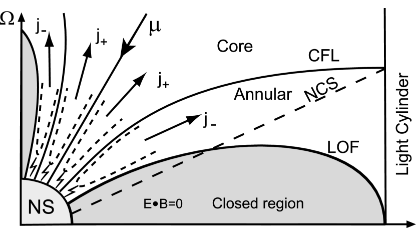
Figure 1: A schematic diagram for the annular and the core regions for an inclined rotator. $\Omega$ and $\mu$ are the rotational and magnetic axis, respectively. The null change surface (NCS) is the surface where the magnetic field is perpendicular to the rotation axis (i.e. ${\rm\bf\Omega\cdot B}=0$). Line ‘CFL’ and ‘LOF’ are the critical field line and the “last” open field line respectively. Charged particles with opposite signs leave off the annular and the core cap regions, respectively. The upper boundaries of the pair formation front are denoted by the dashed lines. The “flash” symbols indicate the locations with the maximal possibility to initiate the pair-production cascade.

For easy discussion in the following, throughout the text we will focus on anti-parallel rotators, i.e. ${\rm\Omega\cdot\mu}<0$. The case of ${\rm\Omega\cdot\mu}>0$ could be derived by reversing the signs, and all the conclusions in this paper remain valid.

For ${\bf\rm\Omega\cdot\mu}<0$, the Goldreich-Julian charge density ($\rho_{\rm{GJ}}$) is positive in the region enclosed by the null charge surface (NCS). For the core-region field lines, positive charges flow out through the light cylinder. The supply of positive charges from the surface compensate the deficit from the light cylinder. To maintain the invariance of the total charge of the pulsar, one needs a current that carries positive charges back to the star, or a current that carries negative charges away from the star. For the fully charge separated magnetosphere, only one sign of charge presents at a given location (Michel, 1979). In the annular region, the negative charged particles at lower altitude can not pass the region with positive GJ charge density at higher altitude. An outer gap then forms beyond the NCS (Holloway, 1973; Krause-Polstorff, Michel, 1985a, b; Smith et al., 2001).

However, resent pulsar magnetosphere simulations presented by some authors (Spitkovsky, 2006; Timokhin, 2006) give different results from that of Smith et al. (2001). Furthermore, there is no a prior justification for a fully charge-separated magnetosphere. Even if the magnetosphere is initially charge-separated, the pair plasma generated from the outer gap will soon fill the annular flux tube, resulting in a quasi-neutral plasma. On the other hand, if one dismisses the conjecture of a fully charge-separated magnetosphere, another natural way to maintain the charge conservation of the pulsar is simply by extracting negative charges directly from the annular polar cap region (for the validity of the picture, see §3.3 for details). In this paper, we explore such a possibility. It is found that the negative charges stripped off from the stellar surface are naturally accelerated in the annular region. This leads to a particle acceleration model that keeps the geometrical advantages of both the polar cap and the outer gap models, which is found suitable to explain the $\gamma$-ray emission data (Dyks, Rudak 2003, Qiao et al. 2004).

Since the positive and the negative charges are accelerated from the core and the annular regions, respectively, the parallel electric fields ($E_{\parallel}$) in the two regions are opposite, as has been discussed by Sturrock (1971) and Holloway (1975). As a result, $E_{\parallel}$ vanishes at the boundary (i.e. critical field lines) between the annular and the core regions. $E_{\parallel}$ also vanishes along the closed field lines. Thus it is equal potential along the closed field lines and the critical field lines. The potential on both the closed field lines and the critical field lines should be equal to the value at infinity. We also assume $E_{\parallel}=0$ at the star surface. When taking into account the $\gamma$-B process for pair production, there exist two accelerators, one at the annular region, and another at the core region. Furthermore, the pair formation front also moves to further distances near the magnetic pole.

One important issue is whether the secondary pairs can screen the $E_{\parallel}$ developed in each region. In the core region, since the primary charge density $\rho$ has the same sign as the $\rho_{\rm GJ}$, the produced secondary pairs tend to get polarized in the acceleration electric field and screen the field. This usually happens especially if the primary $\gamma$-rays are produced through curvature radiation (Harding et al., 2002). For the annular flow, on the other hand, since the primary charge density $\rho$ has the opposite sign with respect to $\rho_{{}_{\rm GJ}}$, one has $\nabla^{2}\Phi\propto(\rho-\rho_{\rm GJ})<0$. As a result, pairs can not screen the acceleration electric field globally. Secondary pairs will be accelerated in the residual electric field. As a result, the charge acceleration region extends from the polar cap to higher locations in the magnetosphere. This potentially matches the geometric model proposed in Qiao et al. (2004). In the following, we will elaborate the idea more quantitatively.

3 Acceleration, pair production and $\gamma$-ray emission

3.1 Primary particle acceleration

In flat space-time, the calculation involving the 1-D Poisson’s equation and the kinetic equation for charges to get the polar gap potential drop was performed by Michel (1974). In the Kerr space-time with small a Lense-Thirring angular velocity, the Poisson’s equation is (Beskin, 1990; Muslimov, Tsygan, 1992).

$$\nabla\cdot(\frac{1}{\sqrt{\kappa}}\bigtriangledown\Phi)=-4\pi(\rho-\rho_{\rm GJ}),$$ (1)

where $\kappa=1-r_{\rm g}/r$, and $r_{\rm g}=2GM/c^{2}$ is the gravitational radius. To the lowest order approximation, one has

$$\rho_{\rm GJ}\simeq-\frac{({\rm\bf\Omega-{\rm\bf\omega}_{\rm LT}})\cdot{\rm\bf B}}{2\sqrt{\kappa}\pi c},$$ (2)

where $\omega_{\rm LT}=0.15\Omega R^{3}r^{-3}I_{45}$ is the local Lense-Thirring angular velocity, and $I_{45}$ is the moment of inertia of the star in unit of $10^{45}\rm g\,cm^{2}$.

In order to reveal the qualitative difference between the annular and the core cap regions (only within the primary accelerator), for simplicity we only solve the 1-dimensional Poisson’s equation

$$\frac{d}{ds}(\frac{1}{\sqrt{\kappa}}\frac{d\Phi}{ds})=-4\pi(\rho-\rho_{\rm GJ})~{}.$$ (3)

This equation is only valid when $s<r_{\rm P}$, but in Fig. 2 a tighter limit is placed. A full 3-D treatment is desirable to fully describe the electrodynamics of the system, and we postpone it to a future work. The 3-D calculation will be reduced to 1-D result, when the solution is confined in a region the transverse size of which is much larger than the longitudinal size, i.e. $\nabla^{2}=\partial^{2}/\partial s_{\rm trans}+\partial^{2}/\partial s_{\rm long}\simeq\partial^{2}/\partial s_{\rm trans}$ for $s_{\rm trans}>>s_{\rm long}$. Neglecting minor energy loss due to radiation, the energy conservation law for particles in a given magnetic flux tube is $\gamma m_{0}c^{2}+q\Phi=m_{0}c^{2}$, where we have used the condition $\Phi=0$ and $E_{\parallel}=0$ at the stellar surface. It should be noted that here the condition $\Phi=0$ at the star surface can only be used in the 1-D calculation and should not be regarded as the boundary condition, since setting any $\Phi$ at the star surface do not change the physical picture. The real physical boundary condition is $E_{\parallel}=0$. This gives $m_{0}c^{2}d\gamma/ds=-qd\Phi/ds$. Here $\gamma$ is the Lorentz factor for the particles; $s$ is the distance along the field line from the stellar surface; and $m_{0},q$ are the mass and the charge of the particles we concern. In the annular region, the primary particles are electrons, so $m_{0}$ and $q$ are the mass and the charge of the electrons. In the core region, $m_{0}$ and $q$ are the mass and charge of the ions pulled out from the surface. In curved space time in the pulsar vicinity, the current conservation law can be expressed as $\sqrt{\kappa}J/B=\sqrt{\kappa}\rho v/B=const$ (for flat space time case it is $\rho v/B=const$), where we assume that the charged particles do not cross magnetic field lines. Here $v$ is the velocity for the particles, and $J=\rho v$ is the current density. The charge density at a given height can be then expressed as $\rho=\sqrt{\kappa}_{0}v_{0}B\rho_{0}/\sqrt{\kappa}vB_{0}$, where the subscript ‘0’ denotes the values at the stellar surface. Submitting the expression of $\rho$ and $\rho_{{}_{\rm GJ}}$ into eq. 3, we get

$$\frac{d}{ds}(\frac{1}{\sqrt{\kappa}}\frac{d}{ds}\gamma) = \chi\lambda^{-2}\left[\chi\frac{Bv_{0}\sqrt{\kappa_{0}}}{B_{0}v\sqrt{\kappa}}-\frac{\rho_{\rm GJ}}{\rho_{\rm GJ0}}\right]$$

$$\lambda^{-2} = \left|\frac{4\pi q\rho_{\rm GJ0}}{m_{\rm 0}c^{2}}\right|,$$ (4)

where $\lambda$ is the reduced Debye wave length for the surface plasma, and a sign parameter $\chi$ is introduced. For ${\rm\bf\Omega\cdot B}<0$, one has $\chi=1,-1$ for the core and the annular regions, respectively. For the $\rm\bf\Omega\cdot B>0$ case, the following calculations are also applicable. The boundary condition at the stellar surface is $\rho=\rho_{{}_{\rm GJ}}$ in the core region, while $\rho=-\rho_{{}_{\rm GJ}}$ in the annular region. The later is based on the consideration that the negative polar cap current would eventually compensate the GJ current loss at the light cylinder.

Equations (3) and (4) are solved numerically for both the core cap (CC) and the annular cap (AC) regions, as presented in Fig. 2. Analytical approximate solutions are also derived. For the core cap, this is $\gamma\simeq 1+\sqrt{2}s/\lambda_{\rm core}$, while for the annular cap it is $\gamma\simeq 1+s^{2}/\lambda_{\rm annular}^{2}$. We see that while the particle Lorentz factor increases linearly in the core region, it increases quadratically in the annular region, analogous to the vacuum gap model (Ruderman, Sutherland, 1975). The analytical solutions are also plotted in Fig. 2, which show very consistent results with the numerical solutions. Notice that in order to compare the difference between the core and the annular regions, we have assumed that the accelerated particles in the core region are positrons. More realistic models involve positively charged ions. This would change the Lorentz factor calculation (lower panel of Fig. 2) by a factor of mass ratio between the positron and the ion.

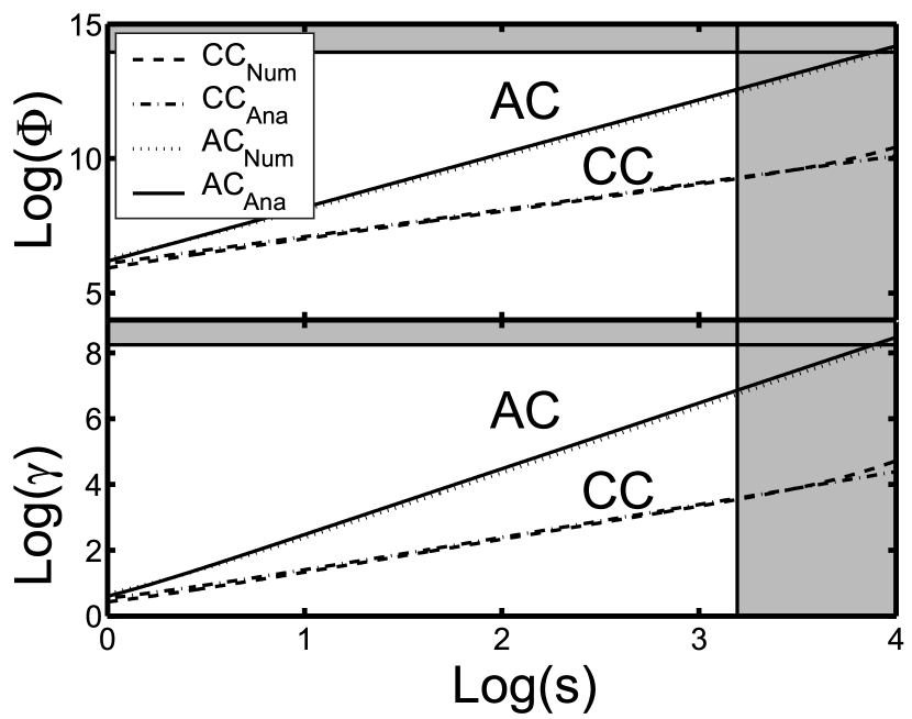
Figure 2: The accelerated potential drop ($\Phi$) and Lorentz factor ($\gamma$) as a function of distance $s$ from stellar surface in the AC and CC for an aligned anti-parallel rotator. $s$ is in units of cm and $\Phi$ is in units of Volt. The legend “AC” and “CC” denote “annular cap” and “core cap”, respectively. The subscripts ’Num’ and ’Ana’ indicate the results from numerical solution and analytic approximation, respectively. The shaded area is the schematic regions where the 1-D annular polar cap acceleration solution is no longer valid. The parameters used here are common values for $\gamma$-ray pulsar (i.e. $p=0.1$ s, $B=10^{12}$ G).

3.2 Location of the pair formation front

The primary particles gain very high Lorentz factors ($\simeq 10^{3}\sim 10^{5}$) within a short distance ($\simeq 10^{2}\simeq 10^{3}$ cm) (Fig. 2). They will radiate $\gamma$-ray photons via curvature radiation and inverse Compton scattering (Ruderman, Sutherland, 1975; Zhang et al., 1997a, b; Harding, 1981; Zhang et al., 2000). The energetic $\gamma$-ray photons will be converted into electron and positron pairs via the $\gamma$-B process. The condition to generate the secondaries is $E_{\rm Mev}B_{\perp 12}/44\geq 1/15$ if the magnetic fields are not close to the critical values (Ruderman, Sutherland, 1975). For curvature radiation, the typical $\gamma$-ray photon energy is $E_{\rm cur}=\frac{2}{3}\frac{c}{\rho}\gamma^{3}\hbar$; for resonant inverse Compton scattering, the typical photon energy is $E_{\rm RICS}=2\hbar\gamma\omega_{\rm B}$, where $\omega_{\rm B}=\frac{eB}{m_{e}c}$ is the cyclotron frequency of electron (Zhang et al., 1997a). The magnetic fields near the stellar surface may not be pure dipolar (Ruderman, Sutherland, 1975; Gil, Melikidze, 2002). We then generically assume that the curvature radius of the magnetic field lines is ${\cal R}$, so that $B_{\perp}=Bs/{\cal R}$, where $B$ is the total magnetic field intensity. One can then estimate the typical length scale of pair production. The typical height of pair formation front (or gap height) in the core region has been estimated previously, e.g. Ruderman, Sutherland (1975); Zhang et al. (1997a, 2000); Harding et al. (2002). Here we focus on the annular region. In the annular cap, one has $\gamma\simeq 1+s^{2}/\lambda^{2}\simeq 0.21s^{2}B_{12}/P$, where $P$ is the pulsar period. Following the method of Zhang et al. (2000), the height of the pair formation front in the annular region can be estimated as

$$h_{\rm Cur} \simeq 4.2\times 10^{3}(\rm cm)\,B_{12}^{-4/7}P^{3/7}{\cal R}_{6}^{2/7}$$

$$h_{\rm RICS} \simeq 2.1\times 10^{4}(\rm cm)\,B_{12}^{-11/7}P^{1/7}{\cal R}_{6}^{4/7}$$ (5)

where the subscripts ’Cur’ and ’RICS’ denote the cases of curvature radiation, and resonant inverse Compton scattering, respectively. We can see that for typical parameters, the pair formation length is in the range of $10^{3}-10^{4}$ cm. Since the solutions for eqs.(3) and (4) are valid only for acceleration of primary particles, the solution breaks above the pair formation front. In Fig. 2 we use a shaded region on the right to denote the region above the pair formation front.

3.3 Secondary pairs

The behavior of the secondary pairs in the core region has been widely discussed. The polarization of the pairs in the initial electric field generates an electric field with the opposite direction to compensate the initial electric field. In most cases, the pair density is so high that the electric field is screened (Harding et al., 2002).

The case of the annular region is different. Whether the particles can be accelerated depends on the electric field direction. If the electric field points towards the star in the annular region, the negative charges will be accelerated outwards and positive charges will be accelerated inwards. The only possibility for the electric field to vanish along the magnetic tube is $\rho=\rho_{\rm GJ}$ associated with trivial boundary condition. But the net free flow from the stellar surface is negative, which is opposite to the local $\rho_{{}_{\rm GJ}}$, thus the electric field can not be globally screened, although it may be partially screened locally and temporarily. The physical picture is that the negative charges move outward on a inward-pointing electric field background (with positive charges moving inward). The inward-pointing electric field is not a new idea. This is in fact discovered very long time ago by Holloway (1973), Cheng , Ruderman(1986), Michel(1979). They proposed the outer gap model, in which the positive charges move inward, which indicates the inward-pointing electric field or at least zero electric field. Since our basic assumption is a quasi-neutral plasma, the negative charges move outward, while positive charges move inward.

An interesting possibility within such a picture is that the annular flow is non-stationary, as has been discussed earlier by Sturrock (1971). This is mainly caused by the interplay between the un-screened electric field and the screening field of the pairs. This may result in oscillating electric fields as envisaged by Levinson et al. (2005), and may provide natural mechanisms to induce pulsar inward emission (Dyks et al., 2005a, b).

3.4 $\gamma$-ray luminosity

The unscreened field extends at least to the NCS. Although with the existence of pairs $E_{\parallel}$ is hard to model, electrons keep accelerating in this extended annular region, and almost achieve the maximum potential drop in the annular cap region, e.g.

$$\Phi_{\rm Max,Ann}=\frac{4\pi^{2}R^{3}B}{cP^{2}}\left[\left(1-\left(\frac{2}{3}\right)^{3/4}\right)+\frac{\alpha}{2}\frac{1}{6^{3/4}}\right]^{2}.$$ (6)

For $\alpha=0$, it is reduced to the value of the aligned rotator (Ruderman, Sutherland, 1975). The maximum particle luminosity from the annular region is $\dot{E}_{\rm ann}=A\rho_{\rm GJ}c\Phi_{\rm Max,Ann}\propto B^{2}P^{-4}(2+\alpha)$, where $A$ is the area of the annular cap region. We can see that the annular cap power is somewhat favorable to stars with large inclination angles. In Fig. 2, eq.(6) is placed as the upper limit of $\Phi$ (denoted by the shaded region above).

An interesting inference from the above picture is that $\gamma$-rays are preferably emitted in the annular flow. Qiao et al. (2004) have investigated such a geometry model, and suggested that the model could well fit the observed wide-beam $\gamma$-ray pulse profiles as well as their radio pulse profiles. The acceleration model proposed in this paper provides the physical basis of that geometric model.

4 Conclusion and discussion

The annular free flow is taken into account in this paper. In the calculation, we assume that $E_{\parallel}=0$ at the star surface and release the assumption that a pulsar magnetosphere must be charge separated. Several conclusions are derived. (1) There are two separate polar cap regions that accelerate particles with opposite signs; (2) Particle acceleration is more facilitated in the annular cap region thanks to its quadratic growth of the electric potential. It is then a favorable source of pair production. (3) Secondary pairs can not screen the parallel electric field in the annular region, so that electrons can be re-accelerated. The acceleration flow may be unsteady. (4) The annular acceleration region extends to the NCS or even beyond it. This leads to a fan-beam $\gamma$-ray emission, which has been found suitable to interpret the observed broad-band emission (Qiao et al. 2004). (5) Both the wide radiation beam observed in the high energy band and the current closure problem for pulsar can be addressed in the same time, if $E_{\parallel}=0$ at star surface is assumed.

Whether the electric field is positive or negative in a given region not only depends on the sign of charges in the region but also the boundary conditions at the surface enclosing the region. Here the electric field is solved in a 1-D model. The potential at the star surface is arbitrarily chosen to be zero and the potential is not a boundary condition. This is not true for 3-D calculations, because the potential at the star surface and potential on the surface of tube is used as the boundary condition. In the SCLF case, boundary condition $\Phi=0$ is actually adopted at the star’s surface, the charges can be accelerated in the charge-depleted region. However the boundary condition $E_{\parallel}=0$ is used at the star surface in our case, so charge excess rather than charge depletion is needed to accelerate particles in the core region. It should be noted that the Possion’s equation is not well posed, if the electric field and the potential are both specified as the boundary conditions at the same places.

The traditional outer gap model is based on the assumption of a fully charge-separated magnetosphere. Our model is based on the different assumption that negative charges are freely supplied from the surface of the pulsar. This leads to a different acceleration picture, in which the $\gamma$-ray emission region can be closer to the null surface. In principle, our model suggests that a vacuum outer gap should not exist.

The re-acceleration and possible pair-production process beyond the pair formation front involves more complicated physics and is subject to further study. A more generalized 3-D treatment for both the core and annular accelerators is desirable.

Both the core and the annular accelerators produce pairs that can emit radio waves. The bi-drifting phenomenon (Champion et al. 2005) can be well interpreted by assuming that the observed radio emission comes from both regions (Qiao et al. 2004b).

If pulsars are bare strange stars (Xu et al., 1999), vacuum gaps would be formed. The separation between the core and the annular region in that model has been discussed in Qiao et al. (2004).

References

- Beskin (1990) Beskin V. S. 1990, Soviet Astronomy Letters, 16, 286
- Champion et al. (2005) Champion D. J., Lorimer D. R., McLaughlin M. A. et al. 2005, MNRAS, 363, 929
- Cheng et al. (1986) Cheng K. S., Ho C., Ruderman M. 1986, ApJ, 300, 500
- Dyks et al. (2005a) Dyks J., Frackowiak M., Slowikowska A., Rudak B., Zhang B. 2005a, ApJ, 633, 1101
- Dyks et al. (2005b) Dyks J., Zhang B., Gil J. 2005b, ApJ, 626, L45
- Dyks, Rudak (2003) Dyks J., Rudak B. 2003, ApJ, 598, 1201
- Fawley et al. (1977) Fawley W. M., Arons J., Scharlemann E. T. 1977, ApJ, 217, 227
- Gil, Melikidze (2002) Gil J., Melikidze G. I. 2002, ApJ, 577, 909
- Gil, Sendyk (2000) Gil J. A., Sendyk M. 2000, ApJ, 541, 351
- Goldreich, Julian (1969) Goldreich P., Julian W. H., 1969, ApJ, 157, 869
- Harding (1981) Harding A. K., 1981, ApJ, 247, 639
- Harding et al. (2002) Harding A. K., Muslimov A. G., Zhang B. 2002, ApJ, 576, 366
- Holloway (1973) Holloway N. J. 1973, Nature, 246, 6
- Holloway (1975) Holloway N. J. 1975, MNRAS, 171, 619
- Krause-Polstorff, Michel (1985a) Krause-Polstorff J., Michel F.C., 1985a,A&A, 144, 72
- Krause-Polstorff, Michel (1985b) Krause-Polstorff J., Michel F.C., 1985b,MNRAS, 213, 43
- Levinson et al. (2005) Levinson A., Melrose D., Judge A., Luo Q. 2005, ApJ, 631, 456
- Michel (1974) Michel F. C., 1974, ApJ, 192, 713
- Michel (1979) Michel F. C., 1979, ApJ, 227, 579
- Michel (1982) Michel F. C., 1982, Rev. Mod. Phys.,54, 1
- Muslimov, Tsygan (1992) Muslimov A. G.,Tsygan A. I. 1992, MNRAS, 255, 61
- Qiao et al. (2004a) Qiao G. J., Lee K. J., Wang H. G., Xu R. X., Han J. L. 2004a, ApJ, 606, L49
- Qiao et al. (2004b) Qiao G. J., Lee K. J., Zhang B., Xu R. X., Wang H. G. 2004b, ApJ, 616, L127
- Ruderman, Sutherland (1975) Ruderman M. A., Sutherland P. G. 1975, ApJ, 196, 51
- Smith et al. (2001) Smith I. A., Michel F. C., Thacker P. D., 2001, MNRAS, 322,209
- Spitkovsky (2006) Spitkovsky A., 2006,ApJ, 648, L51
- Sturrock (1971) Sturrock P. A. 1971, ApJ, 164, 529
- Timokhin (2006) Timokhin A. N., 2006, MNRAS, 368, 1055
- Xu et al. (2006) Xu Ren-Xin, Cui Xiao-Hong, Qiao Guo-Jun 2006, Chin. J. Astron. Astrophys., Vol. 6, No. 2, 217-226
- Xu et al. (1999) Xu R. X., Qiao G. J., Zhang B. 1999, ApJ, 522, L109
- Zhang et al. (1997a) Zhang B., Qiao G. J., Han J. L. 1997a, ApJ, 491, 891
- Zhang et al. (1997b) Zhang B., Qiao G. J., Lin W. P., Han J. L. 1997b, ApJ, 478, 313
- Zhang et al. (2000) Zhang B., Harding A. K., Muslimov A. G. 2000, ApJ, 531, L138