Trapping mechanism in overdamped ratchets with quenched noise

Abstract

A trapping mechanism is observed and proposed as the origin of the anomalous behavior recently discovered in transport properties of overdamped ratchets subject to external oscillatory drive in the presence of quenched noise. In particular, this mechanism is shown to appear whenever the quenched disorder strength is greater than a threshold value. The minimum disorder strength required for the existence of traps is determined by studying the trap structure in a disorder configuration space. An approximation to the trapping probability density function in a disordered region of finite length included in an otherwise perfect ratchet lattice is obtained. The mean velocity of the particles and the diffusion coefficient are found to have a non-monotonic dependence on the quenched noise strength due to the presence of the traps.

I Introduction

The existence of chaotic behavior, which is the seemingly random complex motion observed in deterministic nonlinear systems is now well established. In particular, many approaches have been developed for characterizing and understanding the nature of chaotic motion strogatz .

In addition to chaotic behavior, it has also been shown that deterministic systems can exhibit anomalous transport and strange kinetics scher ; shlesinger ; klafter ; lichtenberg . In analogy with stochastic processes, in the case of normal diffusion geisel ; black , the mean square displacement $<x^{2}>$ is proportional to time $t$ ($<x^{2}>\sim t$), while in the case of strange kinetics shlesinger ; klafter ; barkai , $<x^{2}>\sim t^{\gamma}$, with $\gamma>2$ for enhanced diffusion and $1<\gamma<2$ for dispersive motion. The mean square displacement can also have a logarithmic dependence on time, corresponding to $\gamma=0$ marinari ; krug . Strange kinetics as well as diffusive motion have been observed in both deterministic nonlinear systems morgado ; mallic ; lenzi ; korabel ; kunz as well as thermal ratchets popescu .

In this paper we concentrate on the dynamics of a deterministic thermal ratchet in the presence of a driving force. It has recently been shown popescu that quenched disorder induces a normal diffusive kinetics in addition to the drift due to the external drive. Moreover this diffusive motion is enhanced by higher values of the quenched disorder. If the quenched disorder has long-range spatial correlations, diffusion becomes anomalous, and both the correlation degree and the amount of quenched disorder can enhance the anomalous diffusive transport popescuchin . Anomalous transport has been found recently in overdamped systems linder ; reimann2 . In Linder et al linder an anomalous coherence is reported and P. Reimann et al reimann2 find divergence on the diffusion coefficient. Although our system differs from those previously reported due to the presence of quenched disorder and driving force, the transport anomaly presents some similarities that will be discussed below. While anomalous transport in quenched disorder ratchets was observed for a range of values of the parameters, the mechanism leading to this unusual behavior has not been investigated. Transport properties of ratchets (for a recent review of ratchets, see reimann ) is a topic of great current interest, due to the possible application of these models for understanding such systems as molecular motors Astumian97 ; AstumianHanggi02 , nanoscale friction daikhin ; daly ; soren , surface smoothening baraba , coupled Josephson junctions zapata , as well as mass separation and trapping at the microscale gorre ; deren ; ertas ; duke . The fluctuations that produce the net transport are usually associated with noise, but they may arise also in absence of noise, with additive forcing, in overdamped deterministic systems Barbi7 , overdamped quenched systems popescu and in underdamped ratchets jung ; mateos ; barbi ; quenched2 .

The aim of this paper is to show that a trapping mechanism is responsible for the observed dispersive anomalous transport in an overdamped ratchet subject to an external oscillatory drive motmol . In particular, we show that this mechanism appears when the quenched disorder strength is greater than a threshold value. The minimum disorder strength required for the existence of traps is determined by studying the trap structure in a disorder configuration space. An approximation to the trapping probability density function in a disordered region of finite length included in an otherwise perfect ratchet lattice is obtained. We show that due to this trapping mechanism, the mean velocity of the particles and the diffusion coefficient have a non-monotonic dependence on the quenched noise strength.

The outline of the paper is as follows: in section II we present the single particle model, in section III we define the ensemble and the cumulants, in section IV we present the trapping mechanism and discuss its consequences in section V. Conclusions are presented in section VI.

II Model

The motion of a single particle in an overdamped disordered media is modeled by an overdamped ratchet subject to an external oscillatory drive in the presence of a quenched noise, using the dynamical equation:

$$\gamma\dot{x}=R(x)+F(t)+G(x)$$ (1)

where, $\gamma$ is the damping coefficient, $R(x)=-dU/dx$ is the ratchet force, $F(t)$ is the time dependent external force and $G(x)$ is the quenched disorder force.

The periodic, asymmetric, ratchet potential is modeled by the equation:

$$U(x)=-\sin(x)-\frac{\mu}{2}\sin(2x).$$ (2)

with the spatial period $\lambda=2\pi$, as in previous works popescu ; jung ; mateos ; barbi ; quenched2 ; larro . The external oscillatory force is given by:

$$F(t)=\Gamma\sin(\omega t),$$ (3)

where $\Gamma$ and $\omega$ are the amplitude and the frequency of the oscillations, respectively. The effects of the substrate randomness is modeled by a quenched disorder term of the form:

$$G(x)=\alpha\sum_{i=-\infty}^{\infty}\xi(i)[H(x-i\lambda)-H(x-(i+1)\lambda)],$$ (4)

where the coefficient $\alpha\geq 0$ is the quenched disorder strength, $H$ is the Heaviside function and $\xi(i)$ are independent, uniformly distributed random numbers in $[-1,1]$. The extension to correlated disorder is straightforward. The force $G(x)$ is a piecewise constant force for every period of the ratchet potential and gives a reasonably realistic representation of the effects of the substrate.

In order to carry out a numerical solution of Eq. 1 we have carried out a fourth order fixed step Runge-Kutta method numrec . Since we are interested in the influence of $\Gamma$ and $\alpha$ on the transport properties of the system, the remaining parameters are set to the following values, which were used in previous works popescu ; quenched2 ; motmol ; sincro :

$$\gamma=1;\mu=0.5;\omega=0.1.$$ (5)

We have carried out numerical solutions of the evolution equation using the following dimensionless variables:

• The dimensionless position $\widetilde{x}=x/\lambda$, which gives the position of the particle along the valleys of the ratchet potential.

• The dimensionless velocity $\widetilde{v}=v/v_{\omega}$, with $v_{\omega}=\lambda/T$. The mean value of $\widetilde{v}$ gives the transport velocity of a particle along the ratchet.

• The discrete sequences obtained by sampling $\widetilde{x}$ and $\widetilde{v}$ with a sampling period $T_{sa}=T=2\pi/\omega$:

  $$\widetilde{x}_{sa}=\widetilde{x}(kT)\quad;\quad\widetilde{v}_{sa}=\widetilde{v}(kT)\quad,$$ (6)

  with (k=0,1,2,…). Using these variables it is possible to detect synchronization with the external driving force.

A typical trajectory of Eq. 1 consists of an oscillation superimposed on a directed transport motion with average speed $<\widetilde{v}>$. The particular case of $<\widetilde{v}>=0$ indicates no transport along the ratchet.

In a perfect lattice (i.e. $\alpha=0$) massless particles remain synchronized over the entire $[\Gamma,\omega]$ parameter space sincro . The bifurcation diagrams of $\widetilde{v}_{sa}$ and $<\widetilde{v}>$ as a function of $\Gamma$ are shown in Fig.1 for $\Gamma$ in the range $[0,2]$. Fig.1 shows that $\widetilde{v}_{sa}$ is a monotonic increasing function of $\Gamma$ and $<\widetilde{v}>$ is a stepped function with jumps at specific $\Gamma$ values. The meaning of these jumps may be understood by considering how the particle’s position $\widetilde{x}$ varies as a function of time $\widetilde{t}$. When $\Gamma$ is below 0.96 the particle starts in a potential valley and oscillates inside the valley in synchrony with the external driving force, returning every $T$ to the same position inside the valley. The particle also has the same velocity. This synchronism explains why only one value of $\widetilde{v}_{sa}$ is obtained: at every sampling time the velocity of the particle has the same value within its oscillatory motion.

Over the region $\Gamma\in\left[0.96,1.22\right]$, every $\Gamma$ value has only one value for $\widetilde{v}_{sa}$ but now $<\widetilde{v}>=1$, showing that the particle remains synchronized with the external driving force but now it advances one spatial period (one valley) during $T$. As $\Gamma$ further increases the particle advances 2 valleys, and then 3 valleys during each $T$ (see the labels $(+2,-0)$ and $(+3,-0)$ in Fig.1), giving $<\widetilde{v}>=2$ and $<\widetilde{v}>=3,$ respectively. Furthermore it remains synchronized giving only one value of $\widetilde{v}_{sa}$. If $\Gamma$ further increases, $<\widetilde{v}>$ jumps to a lower value, because during the positive half cycle the particle goes forward, crossing several valleys, but it returns to one or more valleys during the negative half cycle. This explains the labels in Fig. 1. The motion of the particle remains synchronized with the external force through the entire range $\left[0,2\right]$ as it is shown by the single value of $\widetilde{v}_{sa}$.

III Collective Motion

We have studied the evolution of an ensemble of noninteracting particles, uniformly distributed over one whole potential valley. The initial position of the particles is given by the particle density function:

$$\rho(x,0)=[H(\tilde{x}-\tilde{x}_{min})-H(\tilde{x}-\tilde{x}_{max})],$$ (7)

with $\tilde{x}_{max}=\tilde{x}_{min}+1$.

The ensemble was allowed to evolve up to a time $\tilde{t}=1000$, while the positions of the particles were obtained at times $\tilde{t}_{k}=10k$ $(k=0,1,...)$ and stored for further analysis. In order to perform averages over the realizations of disorder a different quenched disorder sequence was used for each trajectory . In this way, the average over the trajectories also includes an average over different realizations of the disorder.

To characterize the evolution of the packet, the first two cumulants,

$$\widetilde{C}_{1}=\left\langle\widetilde{x}_{k}\right\rangle;\text{ }\widetilde{C}_{2}=\left\langle\widetilde{x}_{k}^{2}\right\rangle-\widetilde{C}_{1}^{2};$$ (8)

and their temporal derivatives,

$$\ \langle V\rangle=\lim t\rightarrow\infty\left(d\widetilde{C}_{1}/d\widetilde{t}\right);\text{\ }\widetilde{D}=\lim t\rightarrow\infty\left(d\widetilde{C}_{2}/d\widetilde{t}\right)$$ (9)

were evaluated at the sampling times as a function of time. Here $\langle V\rangle$ is the mean velocity and $\widetilde{D}$ is the diffusion coefficient. In all cases considered, it was verified that all higher-order cumulants increase slower than $t^{n/2}$, ensuring that $\rho(x,t)$ is asymptotically a Gaussian and can be determined using the first two moments only.

IV The trapping mechanism

The superposition of the force $F(t)$, with zero temporal mean, and the force $R(x)$ with a zero spatial mean value, allows the particles to move at different speeds along the potential. Consequently, in spite of the zero spatial mean value of the force $R(x)$ produced by the ratchet potential:

$$\langle R\rangle_{\widetilde{x}}=\frac{1}{N}\int\limits_{\widetilde{x_{1}}}^{\widetilde{x_{1}}+N}R(\widetilde{x})d\widetilde{x}=\frac{1}{N}\left[U\left(\widetilde{x}+N\right)-U\left(\widetilde{x}\right)\right]=0,$$ (10)

the time-averaged mean value felt by the particles is not zero and is given by:

$$\langle R\rangle_{\widetilde{t}}=\frac{1}{N}\int\limits_{\widetilde{t_{1}}}^{\widetilde{t_{1}}+1}R\left[\widetilde{x}\left(\widetilde{t}\right)\right]d\widetilde{t}.$$ (11)

This is in fact the reason a sinusoidal driving force produces a positive drift motion when it is combined with the ratchet potential.

A significant consequence of the quenched disorder is the appearance of a trapping mechanism, which arises only in the disordered case ($\alpha\neq 0$). Traps are a small number of contiguous valleys with a negative time-averaged quenched-disorder mean-value, that exactly compensate the positive time-averaged mean-value of the ratchet potential force. This trapping can be predicted from the synchronization analysis of the perfect lattice case. As an example let us consider the case $\Gamma=1.65$. This $\Gamma$ corresponds to the synchronization zone (+3,-1) in Fig.1. When $\alpha\neq 0$ a particle feels a force that is a combination of the ratchet force plus a sinusoidal force with variable amplitude $\Gamma_{eq}$ between $\Gamma-\alpha$ and $\Gamma+\alpha$. Thus, disorder enables the particle reach different zones, as can be seen in Fig. 1. For example, for $\alpha=0.1$, the available regions for a particle are $(+3,-0)$ and $(+3,-1)$. Then the possible values of $<\widetilde{v}>$ are a result of the combination of the positive and the negative terms: $+3-0=3$ and $+3-1=2$. Thus, $\widetilde{v}$ is bounded between 2 and 3. For $\alpha=\alpha_{z}\simeq 0.175$ the available regions become $(+2,-0)$, $(+3,-0)$, $(+3,-1)$, $(+4,-1)$, and $(+4,-2)$. Then the possible values of $<\widetilde{v}>$ are: $+4-0=4$, $+4-1=3$, $+4-2=2$, $+3-0=3$, $+3-1=2$, $+3-2=1$, $+2-1=1$, $+2-2=0$. Since zero is a possible value, then the particle can be localized or trapped. This corresponds to a particle going forward $2$ valleys during the positive half cycle and going backwards $2$ valleys during the negative half cycle. Consequently, the trapped particle oscillates inside three valleys in synchrony with the external driving force. While this analysis is not exact, it provides a reasonable explanation for both the minimal disorder strength and the corresponding length $K$ in which particles can be trapped.

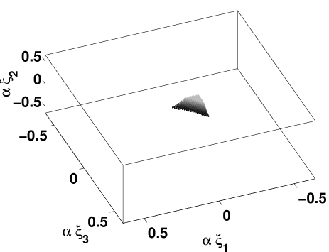
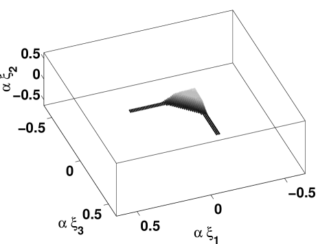
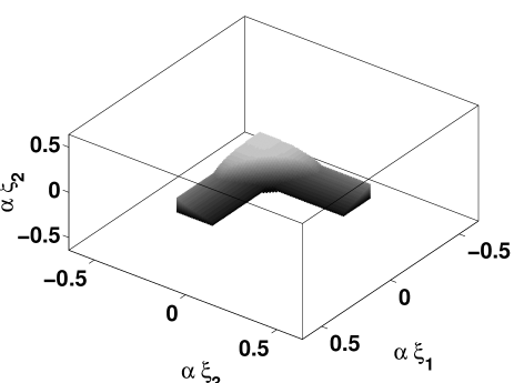
Figure 2: Three dimensional disorder configuration space for $\Gamma=1.65$, $\omega=0.1$, $\gamma=1$ and $\mu=0.5$ as a function of $\alpha$. The axes represent the quenched disorder in three consecutive valleys. The black dots correspond to triplets acting as traps. (a) The case $\alpha=0.20\gtrapprox\beta_{K}$. Note the small trapping region at the corner $\alpha\xi_{1}=\alpha\xi_{2}=\alpha\xi_{3}=-\beta_{K}$, (b) The case $\alpha=0.22\gtrapprox\beta_{K-1}$. Note the appearance of two dimensional arms at $\alpha=\beta_{K-1}$; (c) The case $\alpha=0.30>\beta_{K-1}$

In order to determine the trapping probability, we will first define the quenched disorder forces $G(x)$ of Eq. 1, in one of $K$ consecutive valleys, as the coordinate of a $K$-dimensional disorder configuration space. Possible combinations of disorder are studied in this space and each combination is classified either as a trap or a non-trap. For example for $\Gamma=1.65$ $K=3$; then all possible combinations of three consecutive valleys were studied. The results are shown in a $K=3$ disorder configuration space in Fig. 2. Note that the trapping region in this space changes shape as $\alpha$ increases from 0.2 in Fig. 2(a) to 0.3 in Fig. 2(c). For low values of $\alpha$ there are no traps at all. At a critical value of $\alpha\cong\beta_{K}=\beta_{3}$ the first trap appears (see Fig.2a). Let us call this trap the basic trap as it consists of $K$ consecutive valleys with equal disorder strength (for the case $\Gamma=1,65$, $K=3$ and $\beta_{3}\cong 0.136$).

Note that the volume of the trapping configuration region further increases with increasing $\alpha$ (see Fig. 2b). For $\alpha=\beta_{K-1}=\beta_{2}\cong 0.21$ (see Fig. 2c), two arms appear, corresponding to traps of only $K-1$ consecutive valleys (for the case $\Gamma=1.65$, $K-1=2$). If $\alpha$ is further increased, there exists a higher value $\beta_{K-2}=\beta_{1}$ over which traps of only one valley appear. Note that the minimum $\alpha$ for which traps appear is $\beta_{K}$

When $K=2$, the disorder configuration space is two-dimensional. Traps appear when $\alpha>\beta_{K}=\beta_{2}$. In the interval $\beta_{2}<\alpha<\beta_{1}$, the probability space (that corresponds to trapping events) gradually mutates from a single triangular shape into a square as $\alpha$ grows. When $\alpha>\beta_{1}$, two narrow, rectangle-shaped arms appear, because it is possible now for a particle to get trapped in just one valley. We note that, in Fig. 2, in which a $K=3$ case is considered, the $\beta_{1}$ value is outside the plotting range. If $\beta_{1}$ had been included in the plot three rectangular prisms would have appeared, one for each random variable. For instance, the prism that corresponds to valley number $1$ would have occupied the volume:

$$\begin{pmatrix}-\alpha<\alpha\xi_{1}<-\beta_{1}\\ -\alpha<\alpha\xi_{2}<\alpha\\ -\alpha<\alpha\xi_{2}<\alpha\\ \end{pmatrix}$$ (12)

.

For each $\alpha$ value the cumulative probability of trapping in a $K$-length trap, called $p(\alpha,K)$, is evaluated as the ratio between the volume of the trapping region and $(2\alpha)^{K}$.

When a disordered region of finite length $L>K$ is considered the cumulative probability of trapping is approximately given by:

$$P(\alpha,K,L)=1-Q(\alpha,K,L),$$

$$Q(\alpha,K,L)\cong\left(1-p(\alpha,K)\right)^{L-K+1}.$$ (13)

The approximation used to obtain Eq. IV is based on the assumption that the events of actual trapping of the particle in the neighborhood of the $K$-length traps are independent.

Let $F(\alpha,L)$ be the fraction of particles traversing the length $L$ of the disordered region. We define $f(\alpha,L)$ by the relation:

$$f(\alpha,L)=d\left[1-F(\alpha,L)\right]/d\alpha.$$ (14)

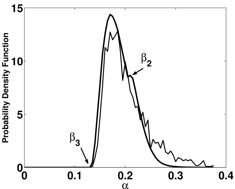
Figure 3: The probability density function $dP(\alpha,K,L)/d\alpha$ from eq. IV (bold curve) and the function $f(\alpha,L)$ from Eq. 14 (thin curve) for $2200$ massless particles traversing a $L=50$ disordered region, are plotted as a function of $\alpha$, for $\Gamma=1.65$,$\gamma=1$, $\omega=0.1$ and $\mu=0.5$.

In Fig. 3, $f(\alpha,L)$ is compared with $dP(\alpha,K,L)/d\alpha$ with the values of $P(\alpha,K,L)$ obtained from Eq. IV. The good agreement between the two results confirms that the independent events approximation used in Eq. IV is clearly valid for $\alpha$ values below $\beta_{K-1}$. Note that the local maximum of both curves in Fig. 3 occurs at $\beta_{K-1}\simeq 0.21$, corresponding to the value at which the ”arms” begin to appear in the disorder-configuration space (see Fig. 2b). We note that the value $\beta_{K-2}\simeq 0.5720$, where $K-2$ valley length traps appear, falls outside the range of the plotted values.

As the disorder region length $L$ grows, the shape of Figure 3 becomes thinner but its left end is still at $\alpha=\beta_{K}$ (in this case, $\alpha=\beta_{3}$). If $L$ tends to infinity the probability that a particle finds a $K$-length trap tends to unity when $\alpha=\beta_{K}$. Then, the shape of figure 3 becomes a Dirac delta function, which is also predicted by Eqs. IV and 14.

We have carried out similar studies for many other values of $\Gamma$ in the range $[0,2]$. We have found that in most of the cases studied, the correlation effects are not important and Eq. IV is accurate enough for determining the probability density function $P(\alpha,K,L)$. There are a few $\Gamma$ values, however, for which the correlation effects cannot be easily neglected, since $\beta_{K}\simeq\beta_{K-1}$ and the ”arms” in the disorder configuration space (like the one in figure 2) appear early on.

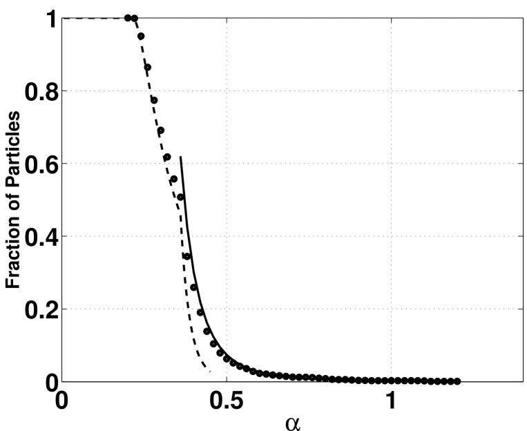
Figure 4: The fraction of particles traversing a length $L=15$ disordered region is plotted as a function of $\alpha$, for $\Gamma=1.35$, $\omega=0.1$, $\gamma=1$ and $\mu=0.5$. Circle markers corresponds to simulations obtained with $1600$ paticles. Dotted line corresponds to function $Q(\alpha,K,L)$ in Eq. IV, where no correlation is considered between contiguous traps. Solid line corresponds to $Q(\alpha,K,L)$ found by using CPM.

As seen in Fig. 4, Eq. IV is not accurate when $\alpha>>\beta_{K}$. This is because the correlations cannot be neglected in this region. We propose another method, which we call the Conditional-Probability Method or CPM, that takes the correlations into account. This method is always accurate provided that $\alpha>>\beta_{1}$ but for some $\Gamma$ values it also works well in the entire $\alpha>\beta_{1}$ range.

Calculations based on CPM involve the following steps: 1) Approximate the probability space volume occupied by trapping events (both black and gray dots in Fig. 3), by a polyhedron in which the faces are perpendicular to the coordinate axes. The $\alpha>\beta_{1}$ case must be considered and rectangle prisms are the main volume component. The smaller volume components are optionally considered, if the method’s range of valid $\alpha$ values is to be increased. If $K=2$ we have a probability space enclosed by a surface with faces that are perpendicular to the coordinate axes. 2) Write the volume equations of the non-trapping events, that is the volume outside the polyhedron, as the union of the set of volumes. The probability of having no traps is proportional to this volume. For example, let us consider the $\Gamma=1.35$ case for which $K=2$. The non-trapping probability $Q(\alpha,K,L)=Q(\alpha,2,2)$ agrees approximately with:

$$Q(\alpha,2,2)(4\alpha^{2})=\begin{pmatrix}-\beta_{1}<\alpha\xi_{1}<\alpha\\ -\beta_{1}<\alpha\xi_{2}<\alpha\end{pmatrix}.$$ (15)

If the smaller surface of trapping events approximately given by

$$-\beta_{1}<\alpha\xi_{1}<-\beta_{2},-\beta_{1}<\alpha\xi_{2}<-\beta_{2}$$ (16)

is taken into account we can instead write:

$$Q(\alpha,2,2)(4\alpha^{2})=\left[\begin{pmatrix}-\beta_{2}<\alpha\xi_{1}<\alpha\\ -\beta_{2}<\alpha\xi_{2}<\alpha\\ \end{pmatrix}\bigcup\begin{pmatrix}-\beta_{2}<\alpha\xi_{1}<\alpha\\ -\beta_{1}<\alpha\xi_{2}<-\beta_{2}\\ \end{pmatrix}\bigcup\begin{pmatrix}-\beta_{1}<\alpha\xi_{1}<-\beta_{2}\\ -\beta_{2}<\alpha\xi_{2}<\alpha\\ \end{pmatrix}\right].$$ (17)

3) Increase $L$, sequentially, in single steps, and find the new volume as the intersection of the previous volumes. That is, $Q(\alpha,K,L-1).(2\alpha)^{(L-1)}$, expanded for all $\alpha\xi_{L}$ and the original $K$-dimensional volume expanded for all $\alpha\xi_{1}$, $\alpha\xi_{2}$, …., $\alpha\xi_{L-K}$ values. Continuing with this procedure and using the most accurate volume equation, we can write the $L=3$ volume in the following way:

$$Q(\alpha,2,3)(8\alpha^{3})=\left[\begin{pmatrix}-\beta_{2}<\alpha\xi_{1}<\alpha\\ -\beta_{2}<\alpha\xi_{2}<\alpha\\ -\alpha<\alpha\xi_{3}<\alpha\\ \end{pmatrix}\bigcup\begin{pmatrix}-\beta_{2}<\alpha\xi_{1}<\alpha\\ -\beta_{1}<\alpha\xi_{2}<-\beta_{2}\\ -\alpha<\alpha\xi_{3}<\alpha\\ \end{pmatrix}\bigcup\begin{pmatrix}-\beta_{1}<\alpha\xi_{1}<-\beta_{2}\\ -\beta_{2}<\alpha\xi_{2}<\alpha\\ -\alpha<\alpha\xi_{3}<\alpha\\ \end{pmatrix}\right]\\ \bigcap\left[\begin{pmatrix}-\alpha<\alpha\xi_{1}<\alpha\\ -\beta_{2}<\alpha\xi_{2}<\alpha\\ -\beta_{2}<\alpha\xi_{3}<\alpha\\ \end{pmatrix}\bigcup\begin{pmatrix}-\alpha<\alpha\xi_{1}<\alpha\\ -\beta_{2}<\alpha\xi_{2}<\alpha\\ -\beta_{1}<\alpha\xi_{3}<-\beta_{2}\\ \end{pmatrix}\bigcup\begin{pmatrix}-\alpha<\alpha\xi_{1}<\alpha\\ -\beta_{1}<\alpha\xi_{2}<-\beta_{2}\\ -\beta_{2}<\alpha\xi_{3}<\alpha\\ \end{pmatrix}\right].$$ (18)

Applying distributive property, the intersection of volumes is computed, yielding:

$$Q(\alpha,2,3)(8\alpha^{3})=\begin{pmatrix}-\beta_{2}<\alpha\xi_{1}<\alpha\\ -\beta_{2}<\alpha\xi_{2}<\alpha\\ -\beta_{2}<\alpha\xi_{3}<\alpha\\ \end{pmatrix}\bigcup\begin{pmatrix}-\beta_{2}<\alpha\xi_{1}<\alpha\\ -\beta_{2}<\alpha\xi_{2}<\alpha\\ -\beta_{1}<\alpha\xi_{3}<-\beta_{2}\\ \end{pmatrix}\bigcup\begin{pmatrix}-\beta_{2}<\alpha\xi_{1}<\alpha\\ -\beta_{1}<\alpha\xi_{2}<-\beta_{2}\\ -\beta_{2}<\alpha\xi_{3}<\alpha\\ \end{pmatrix}\\ \bigcup\begin{pmatrix}-\beta_{1}<\alpha\xi_{1}<-\beta_{2}\\ -\beta_{2}<\alpha\xi_{2}<\alpha\\ -\beta_{2}<\alpha\xi_{3}<\alpha\\ \end{pmatrix}\bigcup\begin{pmatrix}-\beta_{1}<\alpha\xi_{1}<-\beta_{2}\\ -\beta_{2}<\alpha\xi_{2}<\alpha\\ -\beta_{1}<\alpha\xi_{3}<-\beta_{2}\\ \end{pmatrix}.$$ (19)

To find the $L=4$ hyper-volume, the surface in Eq. 17 should be expanded to $4D$, all over $-\alpha<\alpha\xi_{1}<\alpha$, $-\alpha<\alpha\xi_{2}<\alpha$ as follows:

$$\left[\begin{pmatrix}-\alpha<\alpha\xi_{1}<\alpha\\ -\alpha<\alpha\xi_{2}<\alpha\\ -\beta_{2}<\alpha\xi_{3}<\alpha\\ -\beta_{2}<\alpha\xi_{4}<\alpha\\ \end{pmatrix}\bigcup\begin{pmatrix}-\alpha<\alpha\xi_{1}<\alpha\\ -\alpha<\alpha\xi_{2}<\alpha\\ -\beta_{2}<\alpha\xi_{3}<\alpha\\ -\beta_{1}<\alpha\xi_{4}<-\beta_{2}\\ \end{pmatrix}\bigcup\begin{pmatrix}-\alpha<\alpha\xi_{1}<\alpha\\ -\alpha<\alpha\xi_{2}<\alpha\\ -\beta_{1}<\alpha\xi_{3}<-\beta_{2}\\ -\beta_{2}<\alpha\xi_{4}<\alpha\\ \end{pmatrix}\right]$$ (20)

and the volume in Eq. 19 should also be expanded to $4D$ all over $-\alpha<\alpha\xi_{4}<\alpha$. Finally the intersection between these $4D$ hyper-volumes must be found.

As $L$ grows, the number of component hyper-volumes in the set increases and their intersections are hard to calculate by hand. We calculated the resultant hyper-volume up to $L=15$ by using a binary method in which intersections are ’and’ boolean operators. Fig. 4 shows that there is excellent agreement when $\alpha>\beta_{1}$ for $L=15$.

V Connection between Trapping and Transport Properties

The presence of the traps has a significant macroscopic consequence in multiparticle systems on the variation of the current $\langle\widetilde{V}\rangle$ and the diffusion coefficient $\widetilde{D}$. In order to explain this consequence, consider the cumulants $\widetilde{C}_{1}$ and $\widetilde{C}_{2}$, shown in Fig. 5, as a function of time for a packet of $2200$ massless particles with $\Gamma=1.65$, $\omega=0.1$, $\gamma=1$, $L=50$ and $\mu=0.5$. The corresponding derivatives $<\widetilde{V}>$ and $<\widetilde{D}>$, are plotted as a function of $\alpha$ in Figs. 6a - 6c. We note that as a function of $\alpha$, four regions with different transport properties may be recognized in these figures:

1) Very low disorder strength region, $\alpha\leq 0.08$. In this region the disorder has no effect (see the case $\alpha=0.06$ in Fig. 5), the first cummulant $\widetilde{C}_{1}$ is proportional to $\widetilde{t}$ and there is no diffusion as evidenced by the constant value of $\widetilde{C}_{2}$ and the zero value of $<\widetilde{D}>$ (see Fig. 6c). Particles can only reach the region $(+3,-1)$ of Fig. 1 and the only possible value of the mean velocity of the particles is $2$. Thus, $<\widetilde{V}>$ remains constant equal to $2$ and the dynamics is essentially the same as in the perfect lattice case.

2) Intermediate disorder region, $0.08<\alpha<\beta_{K}=0.136$ (see the case $\alpha=0.12$ in Fig. 5 and Fig. 6c, where this region is enlarged). In this region, the first cummulant $\widetilde{C}_{1}$ is proportional to $\widetilde{t}$, but now $\widetilde{C}_{2}\thicksim\widetilde{t}$, indicating the existence of normal diffusion. The slope of the packet mean velocity changes abruptly for each value of $\alpha$, where a new mode is reached, as seen in Fig. 1. At $\alpha>0.08$ the region labeled $(+3,-0)$ is reached and the mean velocity may have one of the two values $+2$ or $+3$. Consequently $\widetilde{V}$ increases with $\alpha$, as can be seen in Fig. 6a. At $\alpha=0.1$ region $(+4,-1)$ is also available and the mean velocity can have any of the values $+2$, $+3$ and $+4$. Then $\widetilde{V}$ continues increasing with $\alpha$, with a higher slope. Fig. 6c shows an enlarged view of a region of Fig. 6b, where the normal diffusion can be observed. As can be seen, for $\alpha<0.08$ transport is not diffusive. At $\alpha=0.08$ normal diffusion starts and as $\alpha$ is increased further, diffusion is enhanced and the same critical value of $\alpha$ appear as in the case of $\widetilde{V}$ (Fig.6a).

3) The region $\alpha\simeq\beta_{K}=0.136$ (see, for example, the case $\alpha=0.145$ in Fig.5). In this region the trapping mechanism has already started. The cumulants $C_{1}$ and $C_{2}$ increase as $\widetilde{t}^{H}$ with $H>1$, indicating a super-diffusive behavior. The time-dependence of the second moment is very complicated during the trapping process and it strongly depends on both the quenched disorder realization and the strength of the disorder. This transitory time is considerably reduced as $\alpha$ increases beyond the threshold. The trapping mechanism produces an abrupt descent in $\widetilde{V}$. The other values $\beta_{K-1}=\beta_{2}$ and $\beta_{K-2}=\beta_{1}$ do not appear in Figs.6 because the probability that a particle gets trapped in a $K=3$ valley length trap approaches $1$ for a disorder region with $L=50>>K=3$, and most particles get trapped in $K=3$ length valleys, regardless of whether $K-1=2$ and $K-2=1$ length traps exist or not. In Fig. 6b the super diffusive region is clearly recognized by the high values in $\widetilde{D}$. Below the threshold value $\beta_{K}$ diffusion is normal and $\widetilde{D}$ is much smaller than in the super diffusive region. Note that $\widetilde{C_{2}}$ varies with time in a very complicated way as long as there exist both, trapped and untrapped particles. Untrapped particles suffer a normal diffusion process but trapped particles cause the packet to get wider as it evolves, increasing $D$. In fact, for $t\rightarrow\infty$ (and consequently $L\rightarrow\infty$) all particles get finally trapped and $D\rightarrow 0$ .

4) The region $\alpha\gg\beta_{K}$ (see the case $\alpha=0.165$ in Fig.5). In this region, complete trapping occurs even for small disordered zones and both $<\widetilde{V}>$ and $\widetilde{D}$ decrease to zero. The system undergoes a transition at $\alpha=\beta_{K}$ between two different transport regimes: for $\alpha<\beta_{K}$ there is normal diffusive transport while for $\alpha>>\beta_{K}$ both transport and diffusion disappear. In the neighborhood of $\alpha=\beta_{K}$ anomalous diffusion is present. The anomalous transport found recently in an overdamped tilted potential model with thermal noise but without quenched disorder and driving force reimann2 , a similar transition between normal diffusive transport is given by the variation of the tilting force $F$ and anomalous diffusion appears near the critical value $F_{c}$.

The anomalous transport effect of trapping is robust under thermal fluctuations in the sense that thermal fluctuation amplitudes of the order of the quenched disorder strength are required to destroy this effect.

VI Conclusions

A novel trapping mechanism is discovered which is proposed as the origin of the anomalous transport in a multi-particle overdamped disordered ratchet. It is found that once a particle reaches a trap it remains localized inside a small region, oscillating synchronously with the external force. By means of the disorder configuration space, critical values for the disorder strengths were determined and the fraction of particles traversing a disordered region were obtained by means of two methods. In the first method, valid for low disorder, the effects of correlations between the contiguous traps were neglected. In the second approach, which is valid for disorder strengths over all the critical values, correlations were considered. The probability density function shows excellent agreement with the simulation data. The trapping mechanism presented here explains the singular behavior of velocity and diffusion with disorder in overdamped ratchets reported in popescu . This analysis may be helpful in the study of other systems exhibiting strange kinetics and also for practical applications such as the design of particle separation techniques in multi-particle systems.

VII Acknowledgments

This work was partially supported by CONICET (PIP 5569), Universidad Nacional de Mar del Plata and ANPCyT (PICT 11-21409 and PICTO 11-495).

VIII Bibliography

,

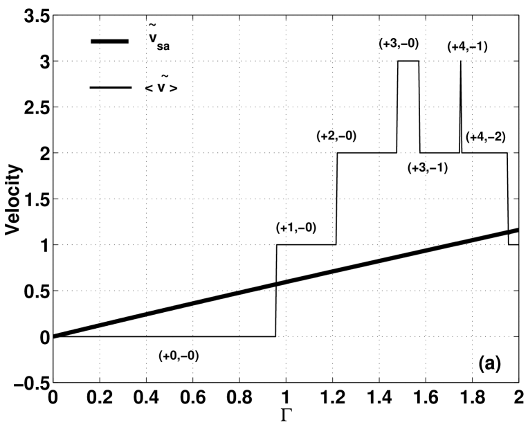
Figure 1: Sampled velocity $\widetilde{v}_{sa}$, and mean velocity $\langle\widetilde{v}\rangle$ of a particle in a perfect lattice, as a function of $\Gamma$. The particle starts at $\widetilde{x}=0$. Note the jumps in $\langle\widetilde{v}\rangle$ at $\Gamma\simeq 0.96,1.22,1.47,1.57,1.75,1.95$, but $\widetilde{v}_{sa}$ has no bifurcations in this range of $\Gamma$. The label over each zone indicates the number of valleys crossed by the particle, forward (+) and backwards (-) in a period $T$.

.

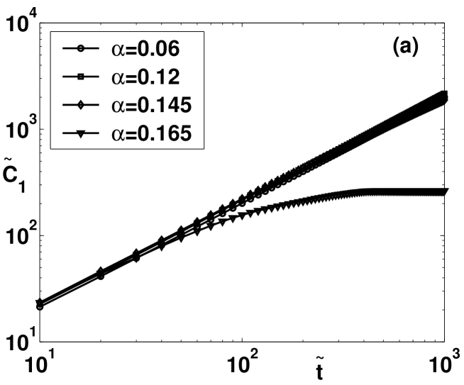
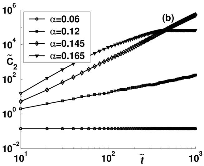
Figure 5: The cumulants (a) $\widetilde{C_{1}}$ and (b) $\widetilde{C_{2}}$ are plotted as a function of time $\widetilde{t}$, for $2200$ massless particles, traversing a $L=50$ disordered region, with $\Gamma=1.65$, $\alpha=0.15$, $\omega=0.1$, $\gamma=1$ and $\mu=0.5$.

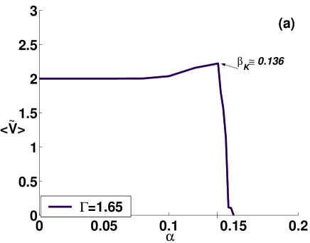
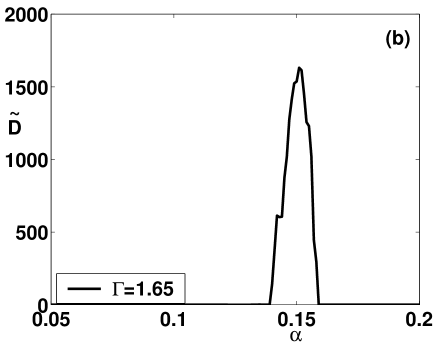
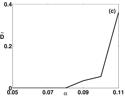
Figure 6: (a) The mean velocity $\langle\widetilde{V}\rangle$ and (b),(c) the diffusion coefficient $\widetilde{D}$ are plotted as a function of $\alpha$ (for a packet of $2200$ particles traversing a $L=50$ disordered region with $\Gamma=1.65$, $\omega=0.1$, $\gamma=1$ and $\mu=0.5$). (c) is an enlargement of part of Fig. (b), where trapping does not exist and the transport is diffusive

References

- (1) S. H. Strogatz, Nonlinear dynamics and chaos: With applications to Physics, Biology, Chemistry, and Engineering. (Addison Wesley, Reading, MA, 1994).
- (2) H. Scher, M. F. Shlesinger and J. T. Bendler, Phys. Today 44, No. 1, 26 (1991).
- (3) M. F. Shlesinger, G. M. Zaslavsky and J. Klafter, Nature (London) 363, 31 (1993).
- (4) J. Klafter, M. F. Shlesinger, and G. Zumofen, Phys. Today 49, No. 2, 33 (1996).
- (5) A. Lichtenberg and M. Lieverman, Regular and Stochastic Motion. (Springer, New York, 1983).
- (6) T. Geisel and J. Nierwetberg, Phys. Rev. Lett. 48, 7 (1982).
- (7) J. A. Blackburn and N. Grønbech-Jensen, Phys. Rev. E 53, 3068 (1996).
- (8) E. Barkai and J. Klafter, Phys. Rev. Lett. 79, 2245 (1997).
- (9) E. Marinari, G. Parisi, D. Ruelle, and P. Windey, Phys. Rev. Lett. 50, 1223 (1983).
- (10) J. Krug and H. T. Dobbs, Phys. Rev. Lett. 76, 4096 (1996).
- (11) R. Morgado, F. A. Olivera, G. G. Batrouni and A. Hansen, Phys. Rev.Lett. 89, 100601/1-4 (2002).
- (12) K. Mallick and P. Marcq, Phys. Rev. E 66, 041113 (2003).
- (13) E. K. Lenzi, R. S. Mendes and C. Tsallis, Phys. Rev. E 67, 031104 (2003).
- (14) N. Korabel and R. Klages, Phys. Rev. Lett. 89, 21402 (2002).
- (15) H. Kunz, R. Livi and A. S, Phys. Rev. E 67, 011102 (2003).
- (16) M. N. Popescu, C. M. Arizmendi, A. L. Salas-Brito and F. Family, Phys. Rev. Lett. 85, 3321 (2000).
- (17) Lei Gao, Xiaoqin Luo, Shiqun Zhu and Bambi Hu, Phys. Rev. E 67, 062104 (2003).
- (18) B. Linder, M. Kostur and L. Schimansky-Geier, Fluctuation and Noise Letters 1, R25 (2001).
- (19) P. Reimann, C. Van den Broeck, H. Linke, P. Hänggi, J. M. Rubi, and A. Pérez-Madrid, Phys. Rev. Lett. 87, 010602 (2001).
- (20) P. Reimann, Physics Reports 361, 57 (2002).
- (21) R. D. Astumian, Science 276, 917 (1997).
- (22) R. D. Astumian and P. Hänggi, Phys. Today 55, 33 (2002).
- (23) L. Daikhin and M. Urbakh, Phys. Rev. E 49, 1424 (1994).
- (24) C. Daly and J. Krim, Phys. Rev. Lett. 76, 803 (1996).
- (25) M. R. Sorensen, K. W. Jacobsen and P. Stoltze, Phys. Rev. B 53, 2101 (1996).
- (26) A. L. Barabási and H. E. Stanley, Fractal Concepts in Surface Growth. (Cambridge University Press, UK, 1995)
- (27) I. Zapata, R. Bartussek, E. Sols and P. Hänggi, Phys.Rev. Lett. 77, 2292 (1996).
- (28) L. Gorre-Talini, J. P. Sspatz and P. Silberzan, Chaos 8, 650 (1998).
- (29) I. Derényi and R. D. Astumian , Phys. Rev. E 58, 7781 (1998).
- (30) D. Ertas, Phys. Rev. Lett. 80, 1548 (1998).
- (31) T. A. J. Duke and R. H. Austin, Phys. Rev. Lett. 80, 1552 (1998).
- (32) P. Hänggi and R. Bartussek Lecture Notes in Physics Vol. 476, ed. J. Parisi et al, (Springer, Berlin, 1996).
- (33) P. Jung, J. G. Kissner and P. Hänggi, Phys. Rev. Lett. 76, 3436 (1996).
- (34) J. L. Mateos, Phys. Rev. Lett. 84, 258 (2000).
- (35) M. Barbi and M. Salerno, Phys. Rev. E 62, 1988 (2000).
- (36) C. M. Arizmendi, F. Family and A. L. Salas-Brito, Phys. Rev. E 63, 061104 (2001).
- (37) F. Family, H. A. Larrondo, D. G. Zarlenga and C. M. Arizmendi, J. Phys.: Condens. Matter 17, S3719 (2005).
- (38) H. A. Larrondo, F. Family and C. M. Arizmendi, Physica A 303, 78 (2002).
- (39) W. H. Press, S. A. Teikolsky, W. T. Vetterling and B. P. Flannery, Numerical Recipes in C. (Cambridge University Press, Cambridge, 1995).
- (40) D. G. Zarlenga, H. A. Larrondo, C. M. Arizmendi and F. Family, Physica A 352, 282 (2005).
,
.