Analytical results for 2-D non-rectilinear waveguides based on the Green’s function

Abstract

We consider the problem of wave propagation for a 2-D rectilinear optical waveguide which presents some perturbation. We construct a mathematical framework to study such a problem and prove the existence of a solution for the case of small imperfections. Our results are based on the knowledge of a Green’s function for the rectilinear case.

1 Introduction

An optical waveguide is a dielectric structure which guides and confines an optical signal along a desired path. Probably, the best known example is the optical fiber, where the light signal is confined in a cylindrical structure. Optical waveguides are largely used in long distance communications, integrated optics and many other applications.

In a rectilinear optical waveguide, the central region (the core) is surrounded by a layer with a lower index of refraction called cladding. A protective jacket covers the cladding. The difference between the indices of refraction of core and cladding makes possible to guide an optical signal and to confine its energy in proximity of the core.

In recent years, the growing interest in optical integrated circuits stimulated the study of waveguides with different geometries. In fact, electromagnetic wave propagation along perturbed waveguides is still continuing to be widely investigated because of its importance in the design of optical devices, such as couplers, tapers, gratings, bendings imperfections of structures and so on.

In this paper we propose an analytical approach to the study of non-rectilinear waveguides. In particular, we will assume that the waveguide is a small perturbation of a rectilinear one and, in such a case, we prove a theorem which guarantees the existence of a solution.

There are two relevant ways of modeling wave propagation in optical waveguides. In closed waveguides one considers a tubular neighbourhood of the core and imposes Dirichlet, Neumann or Robin conditions on its boundary (see [Ol] and references therein). The use of these boundary conditions is efficient but somewhat artificial, since it creates spurious waves reflected by the interface jacket-cladding. In this paper we will study open waveguides, i.e. we will assume that the cladding (or the jacket) extends to infinity. This choice provides a more accurate model to study the energy radiated outside the core (see [SL] and [Ma]).

Thinking of an optical signal as a superposition of waves of different frequency (the modes), it is observed that in a rectilinear waveguide most of the energy provided by the source propagates as a finite number of such waves (the guided modes). The guided modes are mostly confined in the core; they decay exponentially transversally to the waveguide’s axis and propagate along that axis without any significant loss of energy. The rest of the energy (the radiating energy) is made of radiation and evanescent modes, according to their different behaviour along the waveguide’s axis (see §3 for further details). The electromagnetic field can be represented as a discrete sum of guided modes and a continuous sum of radiation and evanescent modes.

As already mentioned, in this paper we shall present an analytical approach to the study of time harmonic wave propagation in perturbed 2-D optical waveguides. As a model equation, we will use the following Helmholtz equation (or reduced wave equation):

$$\Delta u(x,z)+k^{2}n(x,z)^{2}u(x,z)=f(x,z),$$ (1)

with $(x,z)\in\mathbb{R}^{2}$, where $n(x,z)$ is the index of refraction of the waveguide, $k$ is the wavenumber and $f$ is a function representing a source. The axis of the waveguide is assumed to be the $z$ axis, while $x$ denotes the transversal coordinate.

Our work is strictly connected to the results in [MS], where the authors derived a resolution formula for (1), obtained as a superposition of guided, radiation and evanescent modes, in the case in which the function $n$ is of the form

$$n:=n_{0}(x)=\begin{cases}n_{co}(x),&|x|\leq h,\\ n_{cl},&|x|>h,\end{cases}$$ (2)

where $n_{co}$ is a bounded function decreasing along the positive direction and $2h$ is the width of the core. Such a choice of $n$ corresponds to an index of refraction depending only on the transversal coordinate and, thus, (1) describes the electromagnetic wave propagation in a rectilinear open waveguide. By using the approach proposed in [AC], the results in [MS] have been generalized in [Ci1] to the case in which the index of refraction is not necessarily decreasing along the positive direction. The use of a rigorous transform theory guarantees that the superposition of guided, radiation and evanescent modes is complete. Such results are recalled in §3. The problem of studying the uniqueness of the obtained solution and its outgoing nature will be addressed elsewhere.

In this paper we shall study small perturbations of rectilinear waveguides and present a mathematical framework which allows us to study the problem of wave propagation in perturbed waveguides. In particular, we shall assume that it is possible to find a diffeomorphism of $\mathbb{R}^{2}$ such that the non-rectilinear waveguide is mapped in a rectilinear one. Thanks to our knowledge of a Green’s function for the rectilinear case, we are able to prove the existence of a solution for small perturbations of 2-D rectilinear waveguides by using the contraction mapping theorem.

In order to use such theorem, we shall prove that the inverse of the operator obtained by linearizing the problem is continuous (see Theorem 10). Such a problem has been solved by using weighted Sobolev spaces, which are commonly used when dealing with Helmholtz equation (see, for instance, [Le]).

In a forthcoming work, the results obtained in this paper will be used to show several numerical results interesting for the applications.

In §2 we describe our mathematical framework for studying non-rectilinear waveguides. Since our results are based on the knowledge of a Green’s function for rectilinear waveguides, in §3 we recall the main results obtained in [MS].

Section 4 will be devoted to some technical lemmas needed in §5. The existence of a solution for the problem of perturbed waveguides will be proven in Theorem 10. Crucial to our construction are the estimates contained in §5, in particular the ones in Theorem 8.

Appendix A contains results on the global regularity for solutions of the Helmholtz equation in $\mathbb{R}^{N}$, $N\geq 2$, that we need in Theorem 10.

2 Non-rectilinear waveguides: framework description

When a rectilinear waveguide has some imperfection or the waveguide slightly bends from the rectilinear position, we cannot assume that its index of refraction $n$ depends only on the transversal coordinate $x$. From the mathematical point of view, in this case, we shall study the Helmholtz equation

$$\Delta u+k^{2}n_{\varepsilon}(x,z)^{2}u=f,\quad\textmd{in }\mathbb{R}^{2},$$ (3)

where $n_{\varepsilon}(x,z)$ is a perturbation of the function $n_{0}(x)$ defined in (2), representing a “perfect” rectilinear configuration.

We denote by $L_{0}$ and $L_{\varepsilon}$ the Helmholtz operators corresponding to $n_{0}(x)$ and $n_{\varepsilon}(x,z)$ respectively:

$$L_{0}=\Delta+k^{2}n_{0}(x)^{2},\quad L_{\varepsilon}=\Delta+k^{2}n_{\varepsilon}(x,z)^{2}.$$ (4)

In [MS], the authors found a resolution formula for

$$L_{0}u=f,$$

i.e. they were able to write explicitly (in terms of a Green’s function) the operator $L_{0}^{-1}$ and then a solution of (1). Now, we want to use $L_{0}^{-1}$ to write higher order approximations of solutions of (3), i.e. of

$$L_{\varepsilon}u=f.$$ (5)

The existence of a solution of (5) will be proven in Theorem 10 by using a standard fixed point argument: since (5) is equivalent to

$$L_{0}u=f+(L_{0}-L_{\varepsilon})u,$$

then we have

$$u=L_{0}^{-1}f+\varepsilon L_{0}^{-1}\left(\frac{L_{0}-L_{\varepsilon}}{\varepsilon}\right)u.$$

Our goal is to find suitable function spaces on which $L_{0}^{-1}$ and $\frac{L_{0}-L_{\varepsilon}}{\varepsilon}$ are continuous; then, by choosing $\varepsilon$ sufficiently small, the existence of a solution will follow by the contraction mapping theorem.

It is clear that this procedure can be extended to more general elliptic operators; in §5 we will provide the details.

3 A Green’s function for rectilinear waveguides

In this section we recall the expression of the Green’s formula obtained by Magnanini and Santosa in [MS] and generalized in [Ci1] to a non-symmetric index of refraction.

We look for solutions of the homogeneous equation associated to (1) in the form

$$u(x,z)=v(x,\lambda)e^{ik\beta z};$$

$v(x,\lambda)$ satisfies the associated eigenvalue problem for $v$:

$$v^{\prime\prime}+[\lambda-q(x)]v=0,\quad\textmd{in }\mathbb{R},$$ (6)

with

$$n_{*}=\max_{\mathbb{R}}{n},\quad\lambda=k^{2}(n_{*}^{2}-\beta^{2}),\quad q(x)=k^{2}[n_{*}^{2}-n(x)^{2}].$$ (7)

The solutions of (6) can be written in the following form

$$v_{j}(x,\lambda)=\begin{cases}\phi_{j}(h,\lambda)\cos Q(x-h)+\frac{\phi_{j}^{\prime}(h,\lambda)}{Q}\sin Q(x-h),&\text{if }x>h,\\ \phi_{j}(x,\lambda),&\text{if }|x|\leq h,\\ \phi_{j}(-h,\lambda)\cos Q(x+h)+\frac{\phi_{j}^{\prime}(-h,\lambda)}{Q}\sin Q(x+h),&\text{if }x<-h,\\ \end{cases}$$ (8)

for $j=s,a$, with $Q=\sqrt{\lambda-d^{2}}$, $d^{2}=k^{2}(n_{*}^{2}-n_{cl}^{2})$ and where the $\phi_{j}$’s are solutions of (6) in the interval $(-h,h)$ and satisfy the following conditions:

$$\begin{array}[]{cc}\phi_{s}(0,\lambda)=1,&\phi_{s}^{\prime}(0,\lambda)=0,\\ \phi_{a}(0,\lambda)=0,&\phi_{a}^{\prime}(0,\lambda)=\sqrt{\lambda}.\end{array}$$ (9)

The indices $j=s,a$ correspond to symmetric and antisymmetric solutions, respectively.

Remark 1.

(Classification of solutions). The eigenvalue problem (6) leads to three different types of solutions of (1) of the form $u_{\beta}(x,z)=v(x,\lambda)e^{ik\beta z}$.

• Guided modes: $0<\lambda<d^{2}$. It exists a finite number of eigenvalues $\lambda_{m}^{j}$, $m=1,\ldots,M_{j}$, satisfying the equations

  $$\sqrt{d^{2}-\lambda}\;\phi_{j}(h,\lambda)+\phi_{j}^{\prime}(h,\lambda)=0,\quad j\in\{s,a\},$$

  and corresponding eigenfunctions $v_{j}(x,\lambda_{m}^{j})$ which satisfy (6). In this case, $v_{j}(x,\lambda_{m}^{j})$ decays exponentially for $|x|>h$:

  $$v_{j}(x,\lambda_{m}^{j})=\begin{cases}\phi_{j}(h,\lambda_{m}^{j})e^{-\sqrt{d^{2}-\lambda_{m}^{j}}(x-h)},&x>h,\\ \phi_{j}(x,\lambda_{m}^{j}),&|x|\leq h,\\ \phi_{j}(-h,\lambda_{m}^{j})e^{\sqrt{d^{2}-\lambda_{m}^{j}}(x+h)},&x<-h.\end{cases}$$

  In the $z$ direction, $u_{\beta}$ is bounded and oscillatory, because $\beta$ is real.

• Radiation modes: $d^{2}<\lambda<k^{2}n_{*}^{2}$. In this case, $u_{\beta}$ is bounded and oscillatory both in the $x$ and $z$ directions.

• Evanescent modes: $\lambda>k^{2}n_{*}^{2}$. The functions $v_{j}$ are bounded and oscillatory. In this case $\beta$ becomes imaginary and hence $u_{\beta}$ decays exponentially in one direction along the $z$-axis and increases exponentially in the other one.

By using the theory of Titchmarsh on eigenfunction expansions, we can write a Green’s function for (1) as superposition of guided, radiation and evanescent modes:

$$G(x,z;\xi,\zeta)=\sum_{j\in\{s,a\}}\int\limits_{0}^{+\infty}\frac{e^{i|z-\zeta|\sqrt{k^{2}n_{*}^{2}-\lambda}}}{2i\sqrt{k^{2}n_{*}^{2}-\lambda}}v_{j}(x,\lambda)v_{j}(\xi,\lambda)d\rho_{j}(\lambda),$$ (10)

with

$$\langle d\rho_{j},\eta\rangle=\sum_{m=1}^{M_{j}}r_{m}^{j}\eta(\lambda_{m}^{j})+\frac{1}{2\pi}\int\limits_{d^{2}}^{+\infty}\frac{\sqrt{\lambda-d^{2}}}{(\lambda-d^{2})\phi_{j}(h,\lambda)^{2}+\phi_{j}^{\prime}(h,\lambda)^{2}}\eta(\lambda)d\lambda,$$

for all $\eta\in C_{0}^{\infty}(\mathbb{R})$, where

$$r_{m}^{j}=\left[\int\limits_{-\infty}^{+\infty}v_{j}(x,\lambda_{m}^{j})^{2}dx\right]^{-1}=\frac{\sqrt{d^{2}-\lambda_{m}^{j}}}{\sqrt{d^{2}-\lambda_{m}^{j}}\int\limits_{-h}^{h}\phi_{j}(x,\lambda_{m}^{j})^{2}dx+\phi_{j}(h,\lambda_{m}^{j})^{2}}.$$

and where $v_{j}(x,\lambda)$ are defined by (8) (see [Ci1] for further details).

We notice that (10) can be split up into three summands

$$G=G^{g}+G^{r}+G^{e},$$

where

$$G^{g}(x,z;\xi,\zeta)=\sum_{j\in\{s,a\}}\sum_{m=1}^{M_{j}}\frac{e^{i|z-\zeta|\sqrt{k^{2}n_{*}^{2}-\lambda_{m}^{j}}}}{2i\sqrt{k^{2}n_{*}^{2}-\lambda_{m}^{j}}}v_{j}(x,\lambda_{m}^{j})v_{j}(\xi,\lambda_{m}^{j})r_{m}^{j},$$ (11a)

$$G^{r}(x,z;\xi,\zeta)=\frac{1}{2\pi}\sum_{j\in\{s,a\}}\int\limits_{d^{2}}^{k^{2}n_{*}^{2}}\frac{e^{i|z-\zeta|\sqrt{k^{2}n_{*}^{2}-\lambda}}}{2i\sqrt{k^{2}n_{*}^{2}-\lambda}}v_{j}(x,\lambda)v_{j}(\xi,\lambda)\sigma_{j}(\lambda)d\lambda,$$ (11b)

$$G^{e}(x,z;\xi,\zeta)=-\frac{1}{2\pi}\sum_{j\in\{s,a\}}\int\limits_{k^{2}n_{*}^{2}}^{+\infty}\frac{e^{-|z-\zeta|\sqrt{\lambda-k^{2}n_{*}^{2}}}}{2\sqrt{\lambda-k^{2}n_{*}^{2}}}v_{j}(x,\lambda)v_{j}(\xi,\lambda)\sigma_{j}(\lambda)d\lambda,$$ (11c)

with

$$\sigma_{j}(\lambda)=\frac{\sqrt{\lambda-d^{2}}}{(\lambda-d^{2})\phi_{j}(h,\lambda)^{2}+\phi_{j}^{\prime}(h,\lambda)^{2}}.$$ (12)

$G^{g}$ represents the guided part of the Green’s function, which describes the guided modes, i.e. the modes propagating mainly inside the core; $G^{r}$ and $G^{e}$ are the parts of the Green’s function corresponding to the radiation and evanescent modes, respectively. The radiation and evanescent components altogether form the radiating part $G^{rad}$ of $G$:

$$G^{rad}=G^{r}+G^{e}=\frac{1}{2\pi}\sum_{j\in\{s,a\}}\int\limits_{d^{2}}^{+\infty}\frac{e^{i|z-\zeta|\sqrt{k^{2}n_{*}^{2}-\lambda}}}{2i\sqrt{k^{2}n_{*}^{2}-\lambda}}v_{j}(x,\lambda)v_{j}(\xi,\lambda)\sigma_{j}(\lambda)d\lambda.$$ (13)

4 Asymptotic Lemmas

This section contains some lemmas which will be useful in the rest of the paper.

Lemma 2.

Let $q\in L^{1}_{loc}(\mathbb{R})$ and $\lambda_{0}=\min(\lambda_{1}^{s},\lambda_{1}^{a})$, where $\lambda_{1}^{s}$ and $\lambda_{1}^{a}$ are defined in Remark 1. Let $\phi_{j}$, $j\in\{s,a\}$, be defined by (8). Then, the following estimates hold for $x\in[-h,h]$ and $\lambda\geq\lambda_{0}$:

$$|\phi_{j}(x,\lambda)|\leq\Phi_{*},\quad|\phi_{j}^{\prime}(x,\lambda)|\leq\Phi_{*}\sqrt{\lambda},$$ (14)

where

$$\Phi_{*}:=\exp\left\{\frac{1}{2\sqrt{\lambda_{0}}}\int\limits_{-h}^{h}|q(t)|dt\right\}.$$ (15)

Proof.

We consider the function

$$\psi_{j}(x,\lambda)=\phi_{j}^{\prime}(x,\lambda)^{2}+\lambda\phi_{j}(x,\lambda)^{2},$$

and notice that

$$\psi_{j}^{\prime}(x,\lambda)=2q(x)\phi_{j}(x,\lambda)\phi_{j}^{\prime}(x,\lambda),$$

as it follows from (6). By using Young’s inequality, we get that $\psi_{j}$ satisfies

$$\begin{cases}\displaystyle\psi_{j}^{\prime}(x,\lambda)\leq\frac{|q(x)|}{\sqrt{\lambda}}\psi_{j}(x,\lambda),&\\ \psi_{j}(0,\lambda)=\lambda.\end{cases}$$

Therefore, by integrating the above inequality, we obtain that

$$\psi_{j}(x,\lambda)\leq\lambda\exp\left\{\frac{1}{\sqrt{\lambda}}\int\limits_{-h}^{h}|q(t)|dt\right\}\leq\lambda\Phi_{*}^{2},$$

which implies (14). ∎

In the next two lemmas we study the asymptotic behaviour of the function $\sigma_{j}(\lambda)$ as $\lambda\to+\infty$ and $\lambda\to d^{2}$, respectively.

Lemma 3.

Let $\sigma_{j}(\lambda),\ j\in\{s,a\},$ be the quantities defined in (12). The following asymptotic expansions hold as $\lambda\to\infty$:

$$\sigma_{s}(\lambda)=\frac{1}{\sqrt{\lambda-d^{2}}}+\mathcal{O}\left(\frac{1}{\lambda}\right),\quad\sigma_{a}(\lambda)=\frac{1}{\sqrt{\lambda}}+\mathcal{O}\left(\frac{1}{\lambda}\right).$$ (16)

Proof.

By multiplying

$$\phi_{j}^{\prime\prime}(x,\lambda)+[\lambda-q(x)]\phi_{j}(x,\lambda)=0,\quad x\in[-h,h],$$

by $\phi_{j}^{\prime}(x,\lambda)$ and integrating in $x$ over $(0,h)$, we find

$$\phi_{j}^{\prime}(h,\lambda)^{2}-\phi_{j}^{\prime}(0,\lambda)^{2}+(\lambda-d^{2})[\phi_{j}(h,\lambda)^{2}-\phi_{j}(0,\lambda)^{2}]=2\int\limits_{0}^{h}[q(x)-d^{2}]\phi_{j}(x,\lambda)\phi_{j}^{\prime}(x,\lambda)dx.$$

Thus, by using (9), we obtain the following inequalities:

$$\big{|}\phi_{s}^{\prime}(h,\lambda)^{2}+(\lambda-d^{2})\phi_{s}(h,\lambda)^{2}-(\lambda-d^{2})\big{|}\leq 2k^{2}(n_{*}^{2}+n_{cl}^{2})\int\limits_{0}^{h}|\phi_{s}(x,\lambda)\phi_{s}^{\prime}(x,\lambda)|dx,$$

$$\big{|}\phi_{a}^{\prime}(h,\lambda)^{2}+(\lambda-d^{2})\phi_{a}(h,\lambda)^{2}-\lambda\big{|}\leq 2k^{2}(n_{*}^{2}+n_{cl}^{2})\int\limits_{0}^{h}|\phi_{a}(x,\lambda)\phi_{a}^{\prime}(x,\lambda)|dx.$$

The asymptotic formulas (16) follow from the two inequalities above, (12) and the bounds (14) for $\phi_{j}(x,\lambda)$ and $\phi_{j}^{\prime}(x,\lambda)$. ∎

Lemma 4.

Let $\sigma_{j}(\lambda),\ j\in\{s,a\},$ be the quantities defined in (12). The following formulas hold for $\lambda\to d^{2}$:

$$\sigma_{j}(\lambda)=\begin{cases}\displaystyle\frac{\sqrt{\lambda-d^{2}}}{\phi_{j}^{\prime}(h,d^{2})^{2}}+\mathcal{O}\left(\lambda-d^{2}\right),&\text{if }\phi_{j}^{\prime}(h,d^{2})\neq 0,\\ &\\ \displaystyle\frac{1}{\phi_{j}(h,d^{2})^{2}\sqrt{\lambda-d^{2}}}+\mathcal{O}\left(\sqrt{\lambda-d^{2}}\right),&\text{otherwise}.\end{cases}$$ (17)

Proof.

We recall that, if $q\in L^{1}_{loc}(\mathbb{R})$, for $x\in[-h,h]$, $\phi_{s}(x,\lambda)$ and $\phi_{a}(x,\lambda)$ are analytic in $\lambda$ and $\sqrt{\lambda}$, respectively (see [CL]). Thus, in a neighbourhood of $\lambda=d^{2}$, we write

$$\begin{array}[]{cc}\phi(h,\lambda)=\sum\limits_{m=0}^{+\infty}(\lambda-d^{2})^{m}a_{m},&\phi^{\prime}(h,\lambda)=\sum\limits_{m=0}^{+\infty}(\lambda-d^{2})^{m}b_{m},\\ &\\ \phi(h,\lambda)^{2}=\sum\limits_{m=0}^{+\infty}(\lambda-d^{2})^{m}\alpha_{m},&\phi^{\prime}(h,\lambda)^{2}=\sum\limits_{m=0}^{+\infty}(\lambda-d^{2})^{m}\beta_{m},\end{array}$$

where we omitted the dependence on $j$ to avoid too heavy notations.

We notice that $\alpha_{0}=a_{0}^{2}$, $\alpha_{1}=2a_{0}a_{1}$ and the same for $b_{0}$ and $b_{1}$. From (12) we have

$$\begin{split}\sigma_{j}(\lambda)^{-1}&=\sqrt{\lambda-d^{2}}\phi_{j}(h,\lambda)^{2}+\frac{1}{\sqrt{\lambda-d^{2}}}\phi_{j}^{\prime}(h,\lambda)^{2}\\ &=\frac{\beta_{0}}{\sqrt{\lambda-d^{2}}}+\sum\limits_{m=0}^{+\infty}(\lambda-d^{2})^{m+\frac{1}{2}}(\alpha_{m}+\beta_{m+1}).\end{split}$$ (18)

If $\beta_{0}\neq 0$, since $\beta_{0}=b_{0}^{2}$, (17) follows. If $\beta_{0}=0$ we have that the leading term in (18) is $\alpha_{0}+\beta_{1}$. We notice that $\alpha_{0}\neq 0$, otherwise $\phi(x,d^{2})\equiv 0$ for all $x\in\mathbb{R}$. We know that $\beta_{1}=2b_{0}b_{1}=0$, because $b_{0}=0$. Then $\alpha_{0}+\beta_{1}=\alpha_{0}$ and (17) follows. ∎

5 Existence of a solution

Let $\mu:\mathbb{R}^{2}\to\mathbb{R}$ be a positive function. We will denote by $L^{2}(\mu)$ the weighted space consisting of all the complex valued measurable functions $u(x,z)$, $(x,z)\in\mathbb{R}^{2}$, such that

$$\mu^{\frac{1}{2}}u\in L^{2}(\mathbb{R}^{2}),$$

equipped with the natural norm

$$\|u\|_{L^{2}(\mu)}^{2}=\int\limits_{\mathbb{R}^{2}}|u(x,z)|^{2}\mu(x,z)dxdz.$$

In a similar way we define the weighted Sobolev spaces $H^{1}(\mu)$ and $H^{2}(\mu)$. The norms in $H^{1}(\mu)$ and $H^{2}(\mu)$ are given respectively by:

$$\|u\|_{H^{1}(\mu)}^{2}=\int\limits_{\mathbb{R}^{2}}|u(x,z)|^{2}\mu(x,z)dxdz+\int\limits_{\mathbb{R}^{2}}|\nabla u(x,z)|^{2}\mu(x,z)dxdz,$$

and

$$\|u\|_{H^{2}(\mu)}^{2}=\int\limits_{\mathbb{R}^{2}}|u(x,z)|^{2}\mu(x,z)dxdz+\int\limits_{\mathbb{R}^{2}}|\nabla u(x,z)|^{2}\mu(x,z)dxdz+\int\limits_{\mathbb{R}^{2}}|\nabla^{2}u(x,z)|^{2}\mu(x,z)dxdz.$$

Here, $\nabla u$ and $\nabla^{2}u$ denote the gradient and Hessian matrix of $u$, respectively.

In this section we shall prove an existence theorem for the solutions of (5). We will make use of results on global regularity of the solution of (1); such results will be proven in Appendix A.

The proofs in this section and in Appendix A hold true whenever the (positive) weight $\mu$ has the following properties:

$$\begin{array}[]{c}\mu\in C^{2}(\mathbb{R}^{2})\cap L^{1}(\mathbb{R}^{2}),\\ |\nabla\mu|\leq C_{1}\mu,\quad|\nabla^{2}\mu|\leq C_{2}\mu,\ \ \textmd{ in }\mathbb{R}^{2},\end{array}$$ (19)

where $C_{1}$ and $C_{2}$ are positive constants.

In this section, for the sake of simplicity, we will assume that $\mu$ is given by

$$\mu(x,z)=\mu_{1}(x)\mu_{2}(z).$$ (20)

with $\mu_{j}\in L^{\infty}(\mathbb{R})\cap L^{1}(\mathbb{R}),\ j=1,2$. Analogous results hold for every $\mu$ satisfying (19) and such that

$$\mu(x,z)\leq\mu_{1}(x)\mu_{2}(z).$$ (21)

For instance, it is easy to verify that the more commonly used weight function $\mu(x,z)=(1+x^{2}+z^{2})^{-a}$, $a>1$, satisfies (19) and (21).

Before starting with the estimates on $u$, we prove a preliminary result on the boundness of the guided and radiated parts of the Green’s function.

Lemma 5.

Let $G^{g}$ and $G^{r}$ be the functions defined in (11a) and (11b), respectively. Then

$$|G^{g}(x,z;\xi,\zeta)|\leq\Phi_{*}^{2}\sum_{j\in\{s,a\}}\sum_{m=1}^{M_{j}}\frac{r_{m}^{j}}{2\sqrt{k^{2}n_{*}^{2}-\lambda_{m}^{j}}}\,,$$ (22a)

and

$$|G^{r}(x,z;\xi,\zeta)|\leq\max\left\{\frac{1}{2},\ \frac{\Phi_{*}}{4\sqrt{\pi}}\sum_{j\in\{s,a\}}\Upsilon_{j},\ \frac{\Phi_{*}^{2}}{2\pi}\sum_{j\in\{s,a\}}\Upsilon_{j}^{2}\right\}.$$ (22b)

Here,

$$\Upsilon_{j}=\left(\int\limits_{d^{2}}^{k^{2}n_{*}^{2}}\frac{\sigma_{j}(\lambda)}{2\sqrt{k^{2}n_{*}^{2}-\lambda}}d\lambda\right)^{\frac{1}{2}},\quad j\in\{s,a\},$$

where, as in Lemma 2, $\Phi_{*}$ is given by (15).

Proof.

Since $G^{g}$ is a finite sum, from Remark 1 and Lemma 2, it is easy to deduce (22a).

In the study of $G^{r}$ we have to distinguish three different cases, according to whether $(x,z)$ and $(\xi,\zeta)$ belong to the core or not. Furthermore, we observe that $\Upsilon_{j}<+\infty$ as follows form Lemma 4.

Case 1: $x,\xi\in[-h,h]$. From Lemma 2 we have that $v_{j}(x,\lambda)$ are bounded by $\Phi_{*}$. From (11b) we have

$$|G^{r}|\leq\frac{1}{2\pi}\sum_{j\in\{s,a\}}\Phi_{*}^{2}\Upsilon_{j}^{2}.$$

Case 2: $|x|,|\xi|\geq h$. We can use the explicit formula for $v_{j}$ (see (8)) and obtain by Hölder inequality

$$|v_{j}(x,\lambda)|\leq\sqrt{\phi_{j}(h,\lambda)^{2}+Q^{-2}\phi_{j}^{\prime}(h,\lambda)^{2}}=[Q\,\sigma_{j}(\lambda)]^{-\frac{1}{2}}.$$

Therefore we have

$$|G^{r}(x,z;\xi,\zeta)|\leq\frac{1}{2\pi}\sum_{j\in\{s,a\}}\int\limits_{d^{2}}^{k^{2}n_{*}^{2}}\frac{d\lambda}{2\sqrt{\lambda-d^{2}}\sqrt{k^{2}n_{*}^{2}-\lambda}}=\frac{1}{2},$$

and hence (22b) follows.

Case 3: $|x|\leq h$ and $|\xi|\geq h$. We estimate $|v_{j}(x,\lambda)|$ by $\Phi_{*}$ and $v_{j}(\xi,\lambda)$ by $[Q\sigma_{j}(\lambda)]^{-\frac{1}{2}}$, and write:

$$\begin{split}|G^{r}(x,z;\xi,\zeta)|&\leq\frac{1}{2\pi}\Phi_{*}\sum_{j\in\{s,a\}}\int\limits_{d^{2}}^{k^{2}n_{*}^{2}}\frac{1}{2\sqrt{k^{2}n_{*}^{2}-\lambda}}\left[\frac{\sigma_{j}(\lambda)}{Q}\right]^{\frac{1}{2}}d\lambda\\ &\leq\frac{1}{4\pi}\Phi_{*}\sum_{j\in\{s,a\}}\Upsilon_{j}\left(\int\limits_{d^{2}}^{k^{2}n_{*}^{2}}\frac{d\lambda}{\sqrt{\lambda-d^{2}}\sqrt{k^{2}n_{*}^{2}-\lambda}}\right)^{\frac{1}{2}}.\end{split}$$

Again (22b) follows. ∎

In the next lemma we prove estimates that will be useful in Theorem 8.

Lemma 6.

Let $\mu_{1}\in L^{1}(\mathbb{R})$ and $\mu_{2}\in L^{1}(\mathbb{R})\cap L^{2}(\mathbb{R})$. For $j,l\in\{s,a\}$ and $\lambda,\eta\geq k^{2}n_{*}^{2}$, set

$$p_{j,l}(\lambda,\eta)=\int\limits_{-\infty}^{+\infty}v_{j}(x,\lambda)v_{l}(x,\eta)\mu_{1}(x)dx,$$ (23)

and

$$q(\lambda,\eta)=\int\limits_{-\infty}^{+\infty}(e_{\lambda,\eta}\star\mu_{2})(z)\mu_{2}(z)dz,$$ (24)

where $e_{\lambda,\eta}(z)=e^{-|z|(\sqrt{\lambda-k^{2}n_{*}^{2}}+\sqrt{\eta-k^{2}n_{*}^{2}})}$.

Then $p_{j,l}(\lambda,\eta)=0$ for $j\neq l$,

$$p_{j,j}(\lambda,\eta)^{2}\sigma_{j}(\lambda)\sigma_{j}(\eta)\leq 4\|\mu_{1}\|_{1}^{2}\Bigg{(}\Phi_{*}^{2}\sigma_{j}(\lambda)+\frac{1}{\sqrt{\lambda-d^{2}}}\Bigg{)}\Bigg{(}\Phi_{*}^{2}\sigma_{j}(\eta)+\frac{1}{\sqrt{\eta-d^{2}}}\Bigg{)},$$ (25)

and

$$|q(\lambda,\eta)|\leq\min\left(\|\mu_{2}\|_{1}^{2},\frac{\|\mu_{2}\|_{2}^{2}}{\sqrt[4]{\lambda-k^{2}n_{*}^{2}}\sqrt[4]{\eta-k^{2}n_{*}^{2}}}\right).$$ (26)

Proof.

Since $v_{s}$ and $v_{a}$ are, respectively, even and odd functions of $x$, then $p_{j,l}(\lambda,\eta)=0$ for $j\neq l$.

By Hölder inequality, $p_{j,j}(\lambda,\eta)^{2}\leq p_{j,j}(\lambda,\lambda)p_{j,j}(\eta,\eta)$; also, by the formula (8), we obtain

$$\begin{split}|p_{j,j}(\lambda,\lambda)|&\leq 2\int\limits_{0}^{h}|\phi_{j}(x,\lambda)|^{2}|\mu_{1}(x)|dx+2\int\limits_{h}^{+\infty}|v_{j}(x,\lambda)|^{2}|\mu_{1}(x)|dx\\ &\leq 2\Phi_{*}^{2}\int\limits_{0}^{h}|\mu_{1}(x)|dx+\frac{2}{\sqrt{\lambda-d^{2}}\sigma_{j}(\lambda)}\int\limits_{h}^{+\infty}|\mu_{1}(x)|dx,\end{split}$$

and hence (25).

Now we have to estimate $q(\lambda,\eta)$. Firstly we observe that

$$|q(\lambda,\eta)|\leq\int\limits_{-\infty}^{+\infty}\mu_{2}(z)dz\int\limits_{-\infty}^{+\infty}\mu_{2}(\zeta)d\zeta=\|\mu_{2}\|_{1}^{2},$$

which proves part of (26). Furthermore, from Young’s inequality (see Theorem 4.2 in [LL]) and the arithmetic-geometric mean inequality, we have

$$\begin{split}|q(\lambda,\eta)|\leq\|e_{\lambda,\eta}\|_{1}\|\mu_{2}\|_{2}^{2}&=\frac{2\|\mu_{2}\|_{2}^{2}}{\sqrt{\lambda-k^{2}n_{*}^{2}}+\sqrt{\eta-k^{2}n_{*}^{2}}}\\ &\leq\frac{\|\mu_{2}\|_{2}^{2}}{\sqrt[4]{\lambda-k^{2}n_{*}^{2}}\sqrt[4]{\eta-k^{2}n_{*}^{2}}},\end{split}$$

which completes the proof. ∎

Theorem 7.

Let $G$ be the Green’s function (10). Then

$$\|G\|_{L^{2}(\mu\times\mu)}<+\infty.$$ (27)

Proof.

We write $G=G^{g}+G^{r}+G^{e}$, as in (11a)-(11c), and use Minkowski inequality:

$$\|G\|_{L^{2}(\mu\times\mu)}\leq\|G^{g}\|_{L^{2}(\mu\times\mu)}+\|G^{r}\|_{L^{2}(\mu\times\mu)}+\|G^{e}\|_{L^{2}(\mu\times\mu)}.$$ (28)

From Lemma 5 and (19) it follows that

$$\|G^{g}\|_{L^{2}(\mu\times\mu)},\|G^{r}\|_{L^{2}(\mu\times\mu)}<+\infty.$$ (29)

It remains to prove that $\|G^{e}\|_{L^{2}(\mu\times\mu)}<+\infty$. From (20) we have

$$\begin{split}\|G^{e}\|_{L^{2}(\mu\times\mu)}^{2}&=\int\limits_{\mathbb{R}^{2}\times\mathbb{R}^{2}}|G^{e}(x,z;\xi,\zeta)|^{2}\mu_{1}(x)\mu_{2}(z)\mu_{1}(\xi)\mu_{2}(\zeta)dxdzd\xi d\zeta\\ &=\int\limits_{\mathbb{R}^{2}\times\mathbb{R}^{2}}G^{e}(x,z;\xi,\zeta)\overline{G^{e}(x,z;\xi,\zeta)}\mu_{1}(x)\mu_{2}(z)\mu_{1}(\xi)\mu_{2}(\zeta)dxdzd\xi d\zeta;\end{split}$$

hence, thanks to Lemma 6, the definition (11c) of $G^{e}$ and Fubini’s theorem, we obtain:

$$\|G^{e}\|_{L^{2}(\mu\times\mu)}^{2}\leq\frac{1}{16\pi^{2}}\sum_{j,l\in\{s,a\}}\int\limits_{k^{2}n_{*}^{2}}^{+\infty}\int\limits_{k^{2}n_{*}^{2}}^{+\infty}p_{j,l}(\lambda,\eta)^{2}\sigma_{j}(\lambda)\sigma_{l}(\eta)\frac{q(\lambda,\eta)\;d\lambda d\eta}{\sqrt{\lambda-k^{2}n_{*}^{2}}\sqrt{\eta-k^{2}n_{*}^{2}}}.$$

The conclusion follows from Lemmas 6, 3 and 4. ∎

Corollary 8.

Let $u$ be the solution of (1) given by

$$u(x,z)=\int\limits_{\mathbb{R}^{2}}G(x,z;\xi,\zeta)f(\xi,\zeta)d\xi d\zeta,\ \ (x,z)\in\mathbb{R}^{2},$$ (30)

with $G$ as in (10) and let $f\in L^{2}(\mu^{-1})$. Then

$$\|u\|_{H^{2}(\mu)}\leq C\|f\|_{L^{2}(\mu^{-1})},$$ (31)

where

$$C^{2}=\frac{5}{2}+2C_{2}+\left[\frac{3}{2}+4C_{2}+8C_{2}^{2}+(1+4C_{2})k^{2}n_{*}^{2}+2k^{4}n_{*}^{4}\right]\|G\|_{L^{2}(\mu\times\mu)}^{2}.$$ (32)

Proof.

From (30) and by using Hölder inequality, it follows that

$$\begin{split}\|u\|_{L^{2}(\mu)}^{2}&=\int\limits_{\mathbb{R}^{2}}\Big{|}\int\limits_{\mathbb{R}^{2}}G(x,z;\xi,\zeta)f(\xi,\zeta)d\xi d\zeta\Big{|}^{2}\mu(x,z)dxdz\\ &\leq\|f\|_{L^{2}(\mu^{-1})}^{2}\int\limits_{\mathbb{R}^{2}}\int\limits_{\mathbb{R}^{2}}|G(x,z;\xi,\zeta)|^{2}\mu(\xi,\zeta)\mu(x,z)d\xi d\zeta dxdz\\ &=\|f\|_{L^{2}(\mu^{-1})}^{2}\|G\|_{L^{2}(\mu\times\mu)}^{2},\end{split}$$

and then we obtain (31) and (32) from Lemmas 11 and 13. ∎

Remark 9.

In the next theorem we shall prove the existence of a solution of $L_{\varepsilon}u=f$. It will be useful to assume in general that $L_{\varepsilon}$ is of the form

$$L_{\varepsilon}=\sum_{i,j=1}^{2}a_{ij}^{\varepsilon}\partial_{ij}+\sum_{i=1}^{2}b_{i}^{\varepsilon}\partial_{i}+c^{\varepsilon}.$$ (33)

This choice of $L_{\varepsilon}$ is motivated by our project to treat non-rectilinear waveguides. Our idea is that of transforming a non-rectilinear waveguide into a rectilinear one by a change of variables $\Gamma:\mathbb{R}^{2}\to\mathbb{R}^{2}$.

For this reason, we suppose that $\Gamma$ is a $C^{2}$ invertible function:

$$\Gamma(s,t)=(x(s,t),z(s,t)).$$

By setting $w(s,t)=u(x,z)$, a solution $u$ of (1) is converted into a solution $w$ of

$$|\nabla s|^{2}w_{ss}+|\nabla t|^{2}w_{tt}+2\nabla s\cdot\nabla t\;w_{st}+\Delta s\cdot w_{s}+\Delta t\cdot w_{t}+c(s,t)^{2}w=F(s,t),$$ (34)

where $c(s,t)=kn(x(s,t),z(s,t))$ and $F(s,t)=f(x(s,t),z(s,t))$.

If our waveguide is a slight perturbation of a rectilinear one, we may choose $\Gamma$ as a perturbation of the identity map,

$$\Gamma(s,t)=(s+\varepsilon\varphi(s,t),t+\varepsilon\psi(s,t)),$$

and obtain $L_{\varepsilon}w=F$ from (34), where $L_{\varepsilon}$ is given by (33), with

$$a_{ij}^{\varepsilon}=\delta_{ij}+\varepsilon\tilde{a}_{ij}^{\varepsilon},\ i,j=1,2;\quad b_{i}=\varepsilon\tilde{b}_{i}^{\varepsilon},\ i=1,2;\quad c^{\varepsilon}=k^{2}n_{0}(x)^{2}+\varepsilon\tilde{c}^{\varepsilon};$$ (35)

we also may assume that

$$\left[\sum_{i,j=1}^{2}(\tilde{a}_{ij}^{\varepsilon})^{2}\right]^{\frac{1}{2}},\ \left[\sum_{i=1}^{2}(\tilde{b}_{i}^{\varepsilon})^{2}\right]^{\frac{1}{2}},\ |\tilde{c}^{\varepsilon}|\leq K\mu\quad\textmd{in }\mathbb{R}^{2},$$ (36)

for some constant $K$ independent of $\varepsilon$.

Theorem 10.

Let $L_{\varepsilon}$ be as in Remark 9 and let $f\in L^{2}(\mu^{-1})$. Then there exists a positive number $\varepsilon_{0}$ such that, for every $\varepsilon\in(0,\varepsilon_{0})$, equation $L_{\varepsilon}u=f$ admits a (weak) solution $u^{\varepsilon}\in H^{2}(\mu)$.

Proof.

We write

$$L_{\varepsilon}=L_{0}+\varepsilon\tilde{L}_{\varepsilon};$$ (37)

clearly, the coefficients of $\tilde{L_{\varepsilon}}$ are $\tilde{a}_{ij}^{\varepsilon}$, $\tilde{b}_{i}^{\varepsilon}$ and $\tilde{c}^{\varepsilon}$ defined in (35). We can write (37) as

$$u+\varepsilon L_{0}^{-1}\tilde{L}_{\varepsilon}u=L_{0}^{-1}f;$$

$L_{0}^{-1}f$ is nothing else than the solution of (1) defined in (30).

We shall prove that $L_{0}^{-1}\tilde{L}_{\varepsilon}$ maps $H^{2}(\mu)$ continuously into itself. In fact, for $u\in H^{2}(\mu)$, we easily have:

$$\begin{split}\|\tilde{L}_{\varepsilon}u\|_{L^{2}(\mu^{-1})}^{2}&\leq\int\limits_{\mathbb{R}^{2}}\Bigg{[}\sum_{i,j=1}^{2}(\tilde{a}_{ij}^{\varepsilon})^{2}\sum_{i,j=1}^{2}|u_{ij}|^{2}+\sum_{i=1}^{2}(\tilde{b}_{i}^{\varepsilon})^{2}\sum_{i=1}^{2}|u_{i}|^{2}+(\tilde{c}^{\varepsilon})^{2}|u|^{2}\Bigg{]}\mu^{-1}dxdz\\ &\leq K^{2}\|u\|_{H^{2}(\mu)}^{2}.\end{split}$$

Moreover, Corollary 8 implies that

$$\|L_{0}^{-1}f\|_{H^{2}(\mu)}\leq C\|f\|_{L^{2}(\mu^{-1})},$$

and hence

$$\|L_{0}^{-1}\tilde{L}_{\varepsilon}u\|_{H^{2}(\mu)}\leq CK\|u\|_{H^{2}(\mu)}.$$

Therefore, we choose $\varepsilon_{0}=(CK)^{-1}$ so that, for $\varepsilon\in(0,\varepsilon_{0})$, the operator $\varepsilon L_{0}^{-1}\tilde{L}_{\varepsilon}$ is a contraction and hence our conclusion follows from Picard’s fixed point theorem. ∎

6 Numerical results

In this section we show how to apply our results to compute the first order approximation of the solution of the perturbed problem. The example presented here has only an illustrative scope; a more extensive and rigorous description of the computational issues can be found in [Ci1] and [Ci2], where we apply our results to real-life optical devices.

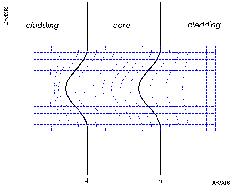
(a) The perturbed waveguide. The dashed lines show the effect of $\Gamma$ on the plane. In particular, they show how a rectangular grid in the $(s,t)$-plane is mapped in the $(x,z)$-plane.

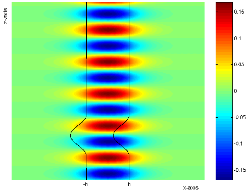
(b) Real part of $w^{(0)}$. Here, $w^{(0)}$ is a pure guided mode supported by the waveguide in the rectilinear configuration.

Figure 1: The perturbed waveguide and the real part of $w^{(0)}$.

In this section we study a perturbed slab waveguide as the one shown in Fig.1(a). In the case of a rectilinear slab waveguide it is possible to write the Green’s formula explicitly and numerically evaluate it (see [MS]).

Having in mind the approach proposed in Remark 9, we change the variables by using a $C^{2}-$function $\Gamma:\mathbb{R}^{2}\to\mathbb{R}^{2}$ of the following form:

$$\Gamma(s,t)=(s,t+\varepsilon S(s)T(t)),$$

where $S,T\in C_{c}^{2}(\mathbb{R})$; a good choice of $S$ and $T$ is represented in Fig.2. In Fig.1(a) we also show how $\Gamma$ transforms the plane, by plotting in the $(x,z)-$plane the image of a rectangular grid in the $(s,t)-$plane.

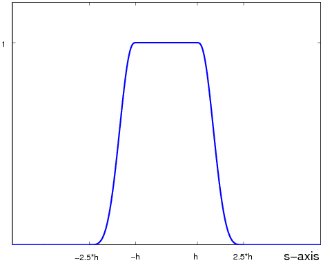
(a) The function $S$.

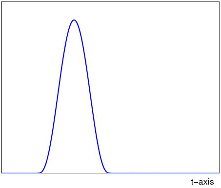
(b) The function $T$.

Figure 2: Our choice of the functions $S$ and $T$. Such a choice corresponds to a perturbed waveguide as in Fig.1(a).

By expanding $L_{\varepsilon}$ and $w$ by their Neumann series, we find that $w^{(0)}$ and $w^{(1)}$ (the zeroth and first order approximations of $w$, respectively) satisfy

$$\Delta w^{(0)}+k^{2}n(s)^{2}w^{(0)}=F(s,t),$$ (38a)

and

$$\Delta w^{(1)}+k^{2}n(s)^{2}w^{(1)}\\ =-2S^{\prime}(s)T(t)w_{ss}^{(0)}-2S(s)T^{\prime}(t)w_{st}^{(0)}-[S^{\prime\prime}(s)T(t)+S(s)T^{\prime\prime}(t)]w_{t}^{(0)},$$ (38b)

respectively.

In our simulations, we assume that $w^{(0)}$ is a pure guided mode and calculate $w^{(1)}$ by using (38) and the Green’s function (10). In other words, we are taking a special choice of $f$ and see what happens to the propagation of a pure guided mode in the presence of an imperfection of the waveguide.

In Figures 1(b), 3 and 4, we set $k=5.0,\,h=0.2,\,n_{co}=2,\,n_{cl}=1$. With such parameters, the waveguide supports two guided modes, corresponding to the following values of the parameter $\lambda$: $\lambda_{1}^{s}=23.7$ and $\lambda_{1}^{a}=73.5$.

As already mentioned, we are assuming that $w^{(0)}$ is a pure guided mode. Here, $w^{(0)}$ is forward propagating and corresponds to $\lambda_{1}^{s}$:

$$w^{(0)}(s,t)=v_{s}(s,\lambda_{1}^{s})e^{it\sqrt{k^{2}n_{*}^{2}-\lambda_{1}^{s}}};$$

the real part of $w^{(0)}$ is shown in Fig.1(b).

Figures 3(a) and 3(b) show the real part and the absolute value of $w^{(1)}$, respectively. We do not write here the numerical details of our computation and refer to [Ci1] and [Ci2] for a more detailed description.

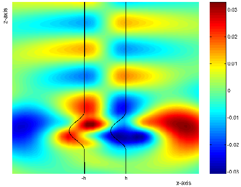
(a) Real part of $w^{(1)}$.

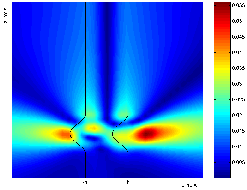
(b) Modulus of $w^{(1)}$.

Figure 3: The real part and modulus of $w^{(1)}$ (the first order approximation of $w$).

In Figures 4(a) and 4(b) we show the real part and the absolute value of $w^{(0)}+\varepsilon w^{(1)}$, respectively. Here, we choose $\varepsilon=1$ to emphasize the effect of the perturbation on the wave propagation. As is clear from Theorem 10, our existence result holds for $\varepsilon\in[0,\varepsilon_{0}]$, where $\varepsilon_{0}=(CK)^{-1}$ (which will be presumably less than $1$). The computation of $\varepsilon_{0}$ and the convergence of the Neumann series related to $w$ have not been considered here; again, we refer to [Ci1] and [Ci2] for a detailed study of such issues.

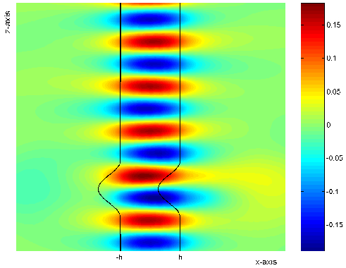
(a) Real part of $w^{(0)}+\varepsilon w^{(1)}$.

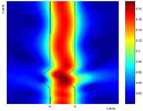
(b) Modulus of $w^{(0)}+\varepsilon w^{(1)}$.

Figure 4: The real part and modulus of $w^{(0)}+\varepsilon w^{(1)}$. The pictures clearly show the effect of a perturbation of the waveguide: due to the presence of an imperfection, the waveguide does not support the pure guided mode $w^{(0)}$ and the other supported guided mode and the radiating energy appear.

7 Conclusions

In this paper, we studied the electromagnetic wave propagation for non-rectilinear waveguides, assuming that the waveguide is a small perturbation of a rectilinear one. Thanks to the knowledge of a Green’s function for the rectilinear configuration, we provided a mathematical framework by which the existence of a solution for the scalar 2-D Helmholtz equation in the perturbed case is proven. Our work is based on careful estimates in suitable weighted Sobolev spaces which allow us to use a standard fix-point argument.

For the case of a slab waveguide (piecewise constant indices of refraction), numerical examples were also presented. We showed that our approach provide a method for evaluating how imperfections of the waveguide affect the wave propagation of a pure guided mode.

In a forthcoming paper, we will address the computational issues arising from the design of optical devices.

Appendix A Regularity results

In this section we study the global regularity of weak solutions of the Helmholtz equation. Since our results hold in $\mathbb{R}^{N}$, $N\geq 2$, it will be useful to denote a point in $\mathbb{R}^{N}$ by $x$, i.e. $x=(x_{1},\ldots,x_{N})\in\mathbb{R}^{N}$.

The results in this section can be found in literature in a more general context for $N\geq 3$ (see [Ag]). Here, under stronger assumptions on $n$ and $\mu$, we provide an ad hoc treatment that holds for $N\geq 2$.

We will suppose $f\in L^{2}(\mu^{-1})$. Since $\mu$ is bounded, it is clear that $f\in L^{2}(\mu)$ too.

Lemma 11.

Let $u\in H^{1}_{\textmd{loc}}(\mathbb{R}^{N})$ be a weak solution of

$$\Delta u+k^{2}n(x)^{2}u=f,\quad x\in\mathbb{R}^{N},$$ (39)

with $n\in L^{\infty}(\mathbb{R}^{N})$. Let $\mu$ satisfy the assumptions in (19). Then

$$\int\limits_{\mathbb{R}^{N}}|\nabla u|^{2}\mu dx\leq\frac{1}{2}\int\limits_{\mathbb{R}^{N}}|f|^{2}\mu dx+\left(2C_{2}+k^{2}n_{*}^{2}+\frac{1}{2}\right)\int\limits_{\mathbb{R}^{N}}|u|^{2}\mu dx,$$ (40)

where $n_{*}=\|n\|_{L^{\infty}(\mathbb{R}^{N})}$.

Proof.

Let $\eta\in C_{0}^{\infty}(\mathbb{R}^{N})$ be such that

$$\eta(0)=1,\quad 0\leq\eta\leq 1,\quad|\nabla\eta|\leq 1,\quad|\nabla^{2}\eta|\leq 1,$$ (41)

and consider the function defined by

$$\mu_{m}(x)=\mu(x)\eta\left(\frac{x}{m}\right).$$ (42)

Then $\mu_{m}(x)$ increases with $m$ and converges to $\mu(x)$ as $m\to+\infty$; furthermore

$$\begin{array}[]{l}\displaystyle|\nabla\mu_{m}(x)|\leq|\nabla\mu(x)|+\frac{1}{m}\mu(x)\leq\left(C_{1}+\frac{1}{m}\right)\mu(x),\\ \displaystyle|\nabla^{2}\mu_{m}(x)|\leq|\nabla^{2}\mu(x)|+\frac{2}{m}|\nabla\mu(x)|+\frac{1}{m^{2}}\mu(x)\leq\left(C_{2}+\frac{2C_{1}}{m}+\frac{1}{m^{2}}\right)\mu(x),\end{array}$$ (43)

for every $x\in\mathbb{R}^{N}$.

Since $u$ is a weak solution of (39), we have that

$$\int\limits_{\mathbb{R}^{N}}\nabla u\cdot\nabla\phi dx-k^{2}\int\limits_{\mathbb{R}^{N}}n(x)^{2}u\phi dx=-\int\limits_{\mathbb{R}^{N}}f\phi dx,$$

for every $\phi\in H^{1}_{\textmd{loc}}(\mathbb{R}^{N})$. We choose $\phi=\bar{u}\mu_{m}$ and obtain by Theorem 6.16 in [LL]:

$$\int\limits_{\mathbb{R}^{N}}|\nabla u|^{2}\mu_{m}dx=-\int\limits_{\mathbb{R}^{N}}\bar{u}\nabla u\cdot\nabla\mu_{m}dx+k^{2}\int\limits_{\mathbb{R}^{N}}n(x)^{2}|u|^{2}\mu_{m}dx-\int\limits_{\mathbb{R}^{N}}f\bar{u}\mu_{m}dx.$$ (44)

Integration by parts gives:

$${\rm{Re}}\int\limits_{\mathbb{R}^{N}}\bar{u}\nabla u\cdot\nabla\mu_{m}dx=-\frac{1}{2}\int\limits_{\mathbb{R}^{N}}|u|^{2}\Delta\mu_{m}dx;$$

hence, by considering the real part of (44), we obtain:

$$\int\limits_{\mathbb{R}^{N}}|\nabla u|^{2}\mu_{m}dx\leq 2\left(C_{2}+\frac{2C_{1}}{m}+\frac{1}{m^{2}}\right)\int\limits_{\mathbb{R}^{N}}|u|^{2}\mu dx+k^{2}n_{*}^{2}\int\limits_{\mathbb{R}^{N}}|u|^{2}\mu_{m}dx\\ +\left(\ \int\limits_{\mathbb{R}^{N}}|f|^{2}\mu_{m}dx\right)^{\frac{1}{2}}\left(\ \int\limits_{\mathbb{R}^{N}}|u|^{2}\mu_{m}dx\right)^{\frac{1}{2}};$$

here we have used (43) and Hölder inequality.

Young inequality and the fact that $\mu_{m}\leq\mu$ then yield:

$$\int\limits_{\mathbb{R}^{N}}|\nabla u|^{2}\mu_{m}dx\leq\left[2\left(C_{2}+\frac{2C_{1}}{m}+\frac{1}{m^{2}}\right)+k^{2}n_{*}^{2}+\frac{1}{2}\right]\int\limits_{\mathbb{R}^{N}}|u|^{2}\mu dx+\frac{1}{2}\int\limits_{\mathbb{R}^{N}}|f|^{2}\mu dx.$$

The conclusion then follows by the monotone convergence theorem. ∎

Lemma 12.

The following identity holds for every $u\in H^{2}_{\textmd{loc}}(\mathbb{R}^{N})$ and every $\phi\in C_{0}^{2}(\mathbb{R}^{N})$:

$$\int\limits_{\mathbb{R}^{N}}|\Delta u|^{2}\phi dx+\int\limits_{\mathbb{R}^{N}}|\nabla u|^{2}\Delta\phi dx=\int\limits_{\mathbb{R}^{N}}|\nabla^{2}u|^{2}\phi dx+{\rm{Re}}\int\limits_{\mathbb{R}^{N}}(\nabla^{2}\phi\nabla u,\nabla u)dx.$$ (45)

Proof.

It is obvious that, without loss of generality, we can assume that $u\in C^{3}(\mathbb{R}^{N})$; a standard approximation argument will then lead to the conclusion.

For $u\in C^{3}(\mathbb{R}^{N})$, (45) follows by integrating over $\mathbb{R}^{N}$ the differential identity

$$\phi\sum_{i,j=1}^{N}u_{ii}\bar{u}_{jj}-\phi\sum_{i,j=1}^{N}u_{ij}\bar{u}_{ij}+\sum_{i,j=1}^{N}u_{i}\bar{u}_{i}\phi_{jj}-{\rm{Re}}\sum_{i,j=1}^{N}u_{i}\bar{u}_{j}\phi_{ij}\\ ={\rm{Re}}\Bigg{\{}\sum_{i,j=1}^{N}\left[(\phi\bar{u}_{j}u_{ii})_{j}+(u_{i}\bar{u}_{i}\phi_{j})_{j}-(\phi\bar{u}_{j}u_{ij})_{i}-(u_{j}\bar{u}_{i}\phi_{j})_{i}\right]\Bigg{\}},$$

and by divergence theorem. ∎

Lemma 13.

Let $u\in H^{1}(\mu)$ be a weak solution of (39). Then

$$\int\limits_{\mathbb{R}^{N}}|\nabla^{2}u|^{2}\mu dx\leq 2\int\limits_{\mathbb{R}^{N}}|f|^{2}\mu dx+2k^{4}n_{*}^{4}\int\limits_{\mathbb{R}^{N}}|u|^{2}\mu dx+4C_{2}\int\limits_{\mathbb{R}^{N}}|\nabla u|^{2}\mu dx.$$ (46)

where $C_{2}$ is the constant in (43).

Proof.

From well-known interior regularity results on elliptic equations (see Theorem 8.8 in [GT]), we have that if $u\in H^{1}_{\textmd{loc}}(\mathbb{R}^{N})$ is a weak solution of (39), then $u\in H^{2}_{\textmd{loc}}(\mathbb{R}^{N})$. Then we can apply Lemma 12 to $u$ by choosing $\phi=\mu_{m}$:

$$\int\limits_{\mathbb{R}^{N}}|\Delta u|^{2}\mu_{m}dx+\int\limits_{\mathbb{R}^{N}}|\nabla u|^{2}\Delta\mu_{m}dx=\int\limits_{\mathbb{R}^{N}}|\nabla^{2}u|^{2}\mu_{m}dx+{\rm{Re}}\int\limits_{\mathbb{R}^{N}}(\nabla^{2}\mu_{m}\nabla u,\nabla u)dx.$$

From (39), (43) and the above formula, we have

$$\begin{split}\int\limits_{\mathbb{R}^{N}}|\nabla^{2}u|^{2}\mu_{m}dx&=\int\limits_{\mathbb{R}^{N}}|f-k^{2}n(x)^{2}u|^{2}\mu_{m}dx+\int\limits_{\mathbb{R}^{N}}|\nabla u|^{2}\Delta\mu_{m}dx-2{\rm{Re}}\int\limits_{\mathbb{R}^{N}}(\nabla^{2}\mu_{m}\nabla u,\nabla u)dx\\ &\leq 2\int\limits_{\mathbb{R}^{N}}|f|^{2}\mu_{m}dx+2k^{4}n_{*}^{4}\int\limits_{\mathbb{R}^{N}}|u|^{2}\mu_{m}dx\\ &\hskip 19.91684pt+2\left(C_{2}+\frac{2C_{1}}{m}+\frac{1}{m^{2}}\right)\int\limits_{\mathbb{R}^{N}}|\nabla u|^{2}\mu dx+2\int\limits_{\mathbb{R}^{N}}|\nabla^{2}\mu_{m}||\nabla u|^{2}dx\\ &\leq 2\int\limits_{\mathbb{R}^{N}}|f|^{2}\mu_{m}dx+2k^{4}n_{*}^{4}\int\limits_{\mathbb{R}^{N}}|u|^{2}\mu_{m}dx\\ &\hskip 19.91684pt+4\left(C_{2}+\frac{2C_{1}}{m}+\frac{1}{m^{2}}\right)\int\limits_{\mathbb{R}^{N}}|\nabla u|^{2}\mu dx.\end{split}$$

Since $\mu_{m}\leq\mu$, the proof is completed by taking the limit as $m\to\infty$. ∎

Acknowledgments

Part of this work was written while the first author was visiting the Institute of Mathematics and its Applications (University of Minnesota). He wishes to thank the Institute for the kind hospitality. The authors are also grateful to Prof. Fadil Santosa (University of Minnesota) for several helpful discussions.

References

[AC]O. Alexandrov and G. Ciraolo,
Wave propagation in a 3-D optical waveguide.
Math. Models Methods Appl. Sci. (M3AS), 14 (2004), no. 6, pp. 819–852.
[Ag]S. Agmon, Spectral Properties of
Schrödinger Operators and Scattering Theory, Ann. Sc. Norm.
Super. Pisa, Cl. Sci., IV. Ser. 2 (1975), pp. 151–218.
[Ci1]G. Ciraolo, Non-rectilinear waveguides: analytical and
numerical results based on the Green’s function, PhD Thesis,
http://www.math.unifi.it/~ciraolo/
[Ci2]G. Ciraolo, A method of variation of boundaries for
waveguide grating couplers, preprint,
http://www.math.unifi.it/~ciraolo/
[CL]E. A. Coddington and N. Levinson, Theory of Ordinary
Differential Equations, McGraw-Hill, New York, 1955.
[GT]D. Gilbarg and N. S. Trudinger, Elliptic partial differential equations of second
order. Springer-Verlag, 1983.
[Le]R. Leis, Initial boundary value problems in mathematical physics,
John Wiley, 1986.
[LL]E. H. Lieb and M. Loss, Analysis, American Mathematical Society, Providence, RI, 1997.
[LS]B. M. Levitan and I. S. Sargsjan, Introduction to spectral theory :
selfadjoint ordinary differential operators. Providence, R.I.,
American Mathematical Society, 1975.
[Ma]D. Marcuse,
Light Transmission Optics, Van Nostrand Reinhold Company, New York, 1982.
[MS]R. Magnanini and F. Santosa,
Wave propagation in a 2-D optical waveguide, SIAM J. Appl.
Math., 61 (2001), pp. 1237–1252.
[Ol]A. A. Oliner, Historical perspectives on microwave field theory, IEEE
Transactions on Microwave Theory and Techniques 32 (1984), no. 9,
pp. 1022–1045.
[SL]A. W. Snyder and D. Love,
Optical Waveguide Theory, Chapman and Hall, London, 1974.
[Ti]E. C. Titchmarsh,
Eigenfunction expansions associated with second-order differential
equations. Oxford at the Clarendon Press, Oxford, 1946.