Fano-Kondo effect through two-level system in triple quantum dots

Abstract

We theoretically study the Fano-Kondo effect in a triple quantum dot (QD) system where two QDs constitute a two-level system and the other QD works in a detector with electrodes. We found that the Fano dip is clearly modulated by strongly coupled QDs in a two-level system and a slow detector with no interacting QD. This setup suggests a new method of reading out qubit states.

I Introduction

Quantum dot (QD) systems have been providing opportunities to probe a wide variety of many-body effects of electronic transport properties in microelectronic structures. The Kondo effect, one of the main characteristics of these systems, is a result of quantum correlation between localized spin in QD and free electrons in electrodesTarucha . Recently, the Fano effect, which appears as a result of quantum interference between a discrete single energy level and a major electronic system, has also attracted the interests of many microelectronics researches. Typically, a dip structure can be observed in conductance plotted as a function of an energy level of a side QDGores ; Sato ; Kang ; Aligia .

A T-shaped QD system consists of two QDs, in which the first QD is connected to a source and a drain and the second QD is set beside the first QD. This system is well suited to investigation of both the Fano effect and Kondo effect (Fano-Kondo effect) and has been theoretically analyzed by many authorsWu ; Guclu ; Tanaka . There are a variety of parameter settings in a T-shaped QD system. Wu et al. assume that there is an infinite on-site Coulomb interaction in the first QD (hereafter we call it ‘detector QD’), and no interaction in the second side-QDWu . On the other hand, Güclü et al. assumes an infinite on-site Coulomb interaction in the second side-QD and no interaction in the detector-QDGuclu . In the former case, Kondo peak is dominant, whereas in the latter case, Fano dip structure is dominant in the transport properties of such a system. Tanaka et al. assume infinite on-site Coulomb interactions in both the detector-QD and the side-QD, showing that Fano dip structure appears in the middle of Kondo resonance peakTanaka .

Here we theoretically investigate the Fano-Kondo effect in a triple QD system, depicted in Fig. 1. When two QDs are coupled, the energy levels mix, and bonding and anti-bonding states are formed. Thus, it is expected that the current that flows through the detector-QD reflects these electronic states when coupling ratio $t_{C}/t_{d}$ is sufficiently large, and the Fano dip would thus be modulated due to this two-level system. We can also regard this setup as an extra impurity connected to a T-shaped QD system, or a charge qubit closely attached to a QD detector. Coupled QDs can be used as a charge qubittana0 ; Goan ; Korotkov ; tanahu ; Gilad . Charge qubits are usually capacitively coupled to detectors that are switched on only after quantum computation is finished. Results of quantum computation are readout through the field-effect (Coulomb interaction) depending on the positions of electrons in the charge qubittana0 ; Goan ; Korotkov ; tanahu ; Gilad . If transfer of an electron between a charge qubit and a detector is not prohibited ($t_{d}\neq 0$) as in the present setup, detector current is expected to be changed by the Fano-Kondo effect. This is an alternative method for reading out the quantum state of the charge qubit, although this method might change the quantum state of qubit more than the previous one, because detector electrons go through the charge qubit directly. To operate a coupled QD system as a charge qubit, we have to maintain the electronic state of the two QDs near the degeneracy point of charging energy, or hold the total number of excess electrons in the charge qubit to one. These requirements lead to stronger constraints on this system. Here, as a first step, we consider only an effect of a two-level system without discussing qubit behaviors.

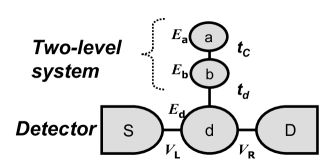
Figure 1: Schematic plot of QD system. QDs $a$ and $b$ constitute a two-level system that is coupled to QD $d$ only which is connected to the electrodes. We consider two cases with differing on the strength of on-site Coulomb interaction in QD $d$. In case I, there is no on-site Coulomb interaction in QD $d$. In case II, there is infinite on-site Coulomb interaction in QD $d$.

A. W. Rushforth et al. experimentally investigated the Fano-Kondo effect when there are two side QDs near the electronic transport regionRushforth . They showed that Fano dip is modulated by the path of electrons through two side QDs. Compared with a simple T-shaped QD system, there are more parameters in this system due to the existence of extra QD. Correspondingly, the Fano-Kondo effect in this system is expected to show more variety of dip behaviors than that in the T-shaped QDs as shown in Ref.Rushforth ; Sasaki . To make the problem transparent without loss of generality, we assume that there is a single energy level in each QD and that the two energy levels of the QD $a$ and QD $b$ coincide and correspond to gate voltages that are applied to those QDs. For convenience, hereafter we call QD $a$ and $b$ a “two-level system”. We mainly investigate the change of conductance as a function of the gate bias.

We use slave boson mean field theory (SBMFT) with the help of nonequilibrium Keldysh Green’s functions. The formulation of SBMFT is very useful and a good starting point to study the transport properties of a strongly correlated QD system. Thus, this method is widely used, although it is only usable at a lower temperature ($T$) region than the Kondo temperature $T_{K}$Newns ; Lopez , that is $T<T_{K}$. Here, we investigate two cases differing in the amount of Coulomb interaction in QD $d$. In case I, there is no Coulomb interaction ($U_{d}=0$) and in case II, there is an infinite Coulomb interaction ($U_{d}=\infty$). The case I experimentally corresponds to a large QD $d$ and the case II corresponds to a small QD $d$. It is expected that we can see clear Fano effect in case I, and a Kondo resonance peak strongly changes Fano dip in case II. Actually, it will be shown that, in order to see the effects of bonding-antibonding states in the detector current, coupling between the two side QDs should be strong and the detector should be sufficiently slow only in case I.

II Formulation

The Hamiltonian for the case II is different from that for the case I in that the former has an additional constraint on QD $d$. The mean field Hamiltonian for the case II is described in terms of slave bosons $b_{\alpha_{1}}$ $(\alpha_{1}=a,b,d)$ as:

$$H^{\rm(II)}=\sum_{\alpha=L,R}\sum_{k_{\alpha},s}E_{k_{\alpha}}c_{k_{\alpha}s}^{\dagger}c_{k_{\alpha}s}+\sum_{\alpha_{1}=a,b,d}\sum_{s}E_{\alpha_{1}}f_{\alpha_{1}s}^{\dagger}f_{\alpha_{1}s}+\sum_{\alpha_{1}=a,b,d}\lambda_{\alpha_{1}}\left(\sum_{s}f_{\alpha_{1}s}^{\dagger}f_{\alpha_{1}s}+b_{\alpha_{1}}^{\dagger}b_{\alpha_{1}}-1\right)$$ (1)

$$+ \!\frac{t_{C}}{N}\sum_{s}(f_{as}^{\dagger}b_{a}b_{b}^{\dagger}f_{bs}+f_{bs}^{\dagger}b_{b}b_{a}^{\dagger}f_{as})+\frac{t_{d}}{N}\sum_{s}(f_{ds}^{\dagger}b_{d}b_{b}^{\dagger}f_{bs}+f_{bs}^{\dagger}b_{b}b_{d}^{\dagger}f_{ds})+\sum_{\alpha=L,R}\frac{V_{\alpha}}{\sqrt{N}}\sum_{k_{\alpha},s}(c_{k_{\alpha}s}^{\dagger}b_{d}^{\dagger}f_{ds}+f_{ds}^{\dagger}b_{d}c_{k_{\alpha}s})$$

where $E_{k_{\alpha}}$ is the energy level for source ($\alpha=L$) and drain ($\alpha=R$) electrodes. $E_{a}$, $E_{b}$ and $E_{d}$ are energy levels for the triple QDs, respectively. $t_{C}$, $t_{d}$ and $V_{\alpha}$ are the tunneling coupling strength between QD $a$ and QD $b$, that between QD $b$ and QD $d$, and that between QD $d$ and electrodes, respectively. $c_{k_{\alpha}s}$ and $f_{\alpha_{1}s}$ are annihilation operators of the electrodes, and of the triple QDs $(\alpha_{1}=a,b,d)$, respectively. $s$ is spin degree of freedom with spin degeneracy $N$; here we apply $N=2$. $\lambda_{\alpha_{1}}$ is a Lagrange multiplier. We take $z_{\alpha_{1}}\equiv b_{\alpha_{1}}^{\dagger}b_{\alpha_{1}}/2$ and $\tilde{E}_{\alpha_{1}}\equiv E_{\alpha_{1}}+\lambda_{\alpha_{1}}$ as mean field parameters. The Hamiltonian for case I is similar to $H^{\rm(II)}$ except that $\lambda_{d}=0$ and $b_{d}=1$ in Eq.(1).

By applying a conventional procedureNewns ; Lopez to this Hamiltonian, we derive Green’s functions for QDs, for example, $G_{dd}^{r}(\omega)=D_{ab}/B_{00}$ etc., where $D_{ab}\equiv(\omega-\tilde{E}_{a})(\omega-\tilde{E}_{b})-\tilde{t}_{C}^{2}$, $B_{00}\equiv{D_{ab}B_{r}-(\omega-\tilde{E}_{a})|\tilde{t}_{d}|^{2}}$ and $B_{r}\equiv\omega-\tilde{E}_{d}+i\Gamma$ with $\tilde{t}_{C}=t_{C}b_{a}b_{b}^{\dagger}/N$ and $\tilde{t}_{d}=t_{d}b_{d}b_{b}^{\dagger}/N$ (see Appendix). Here, $\Gamma_{\alpha}\equiv 2\pi\rho_{\alpha}(E_{F})|V_{\alpha}|^{2}$ is the tunneling rate between $\alpha$ electrode and QD $d$ with a density of states (DOS), $\rho_{\alpha}(E_{F})$, for each electrode at Fermi energy $E_{F}$. $\Gamma\equiv(\Gamma_{L}+\Gamma_{R})/2$ and we assume $\Gamma_{L}=\Gamma_{R}$.

Four self-consistent equations for case I are given.

$$\tilde{t}_{C}\sum_{s}\langle f_{bs}^{\dagger}f_{as}\rangle\!+\!\lambda_{a}|b_{a}|^{2}=0,$$ (2)

$$\tilde{t}_{C}\sum_{s}\langle f_{as}^{\dagger}f_{bs}\rangle+\tilde{t}_{d}\sum_{s}\langle f_{ds}^{\dagger}f_{bs}\rangle\!+\!\lambda_{b}|b_{b}|^{2}=0,$$ (3)

$$\sum_{s}\langle f_{\alpha_{1}s}^{\dagger}f_{\alpha_{1}s}\rangle+|b_{\alpha_{1}}|^{2}=1,\ \ (\alpha_{1}=a,b),$$ (4)

For case II, we have to add two more equations regarding constraints on QD $d$ with $\tilde{V}_{\alpha}=V_{\alpha}b_{d}/\sqrt{N}$:

$$\tilde{t}_{d}^{*}\sum_{s}\langle f_{bs}^{\dagger}f_{ds}\rangle\!\!\! + \!\!\!\!\!\!\!\sum_{\alpha=L,R}\sum_{k_{\alpha},s}\tilde{V}_{\alpha}^{*}\langle c_{k_{\alpha}s}^{\dagger}f_{ds}\rangle\!+\!\lambda_{d}|b_{d}|^{2}\!=\!0$$ (5)

$$\sum_{s}\langle f_{ds}^{\dagger}f_{ds}\rangle + |b_{d}|^{2}=1.$$ (6)

To see the Fano-Kondo effect, we calculate conductance $G\equiv dI_{L}/dV$ at zero bias $V=0$. Source current $I_{L}$ is calculated from Green’s functions as $I_{L}=\frac{e}{\hbar}\int\frac{d\omega}{\pi}\frac{|D_{ab}|^{2}z_{d}^{2}}{B_{00}}\Gamma_{R}\Gamma_{L}(f_{L}(\omega)-f_{R}(\omega))$ with $f_{L}(\omega)\equiv[\exp((\omega+eV)/T)+1]^{-1}$ and $f_{R}(\omega)\equiv[\exp(\omega/T)+1]^{-1}$. Then, we obtain a conductance formula:

$$G=-\frac{e}{\hbar}\int\frac{d\omega}{\pi}\frac{|D_{ab}|^{2}z_{d}^{2}}{B_{00}}\Gamma_{R}\Gamma_{L}\frac{\partial f_{L}(\omega)}{\partial\omega}$$ (7)

The ratio $t_{C}/t_{d}$ compares the internal coupling strength in a two-level system with that between the two-level system and the detector. Here, we regard the case where $t_{C}/t_{d}=5$ as a strongly coupled two-level system and the case where $t_{C}/t_{d}=1$ as a weakly coupled two-level system. Because $\Gamma_{L}\Gamma_{R}/(\Gamma_{L}+\Gamma_{R})$ ($=\Gamma$ ; we assume $\Gamma_{L}=\Gamma_{R}$) can be approximately estimated as a tunneling rate through the detector, if $\Gamma/t_{d}$ is sufficiently large, the electron that flows through QD $d$ is so fast that it cannot detect the oscillation of an electron in the coupled QDs $a$ and $b$. In contrast, if $\Gamma/t_{d}$ is small, the electron that flows through QD $d$ can observe the oscillation between bonding and antibonding states. Therefore, we call a detector with large $\Gamma/t_{d}=2$ a fast detector, and one with smaller $\Gamma/t_{d}=0.4$ a slow detector. $T_{K}$ is estimated as $T_{K}\sim De^{-\pi|\tilde{E}_{d}-E_{F}|/\Gamma}$ $\sim 1.6t_{d}$ ($D$ is a bandwidth), when we assume that $D=20t_{d}$, $|E_{d}|<0.4t_{d}$, $\Gamma>0.4t_{d}$ and $E_{F}=0$.

III Numerical calculations

Here, we numerically investigate the transport properties of our triple QD system for case I ($U_{d}=0$) and case II ($U_{d}=\infty$).

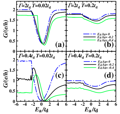
Figure 2: Conductance $G$ as a function of an energy level of the two-level system $E_{a}(=E_{b})$ with a strong coupling ($t_{C}/t_{d}=5$) in case I ($U_{d}=0$). (a) $T/t_{d}=0.02$ and (b) $T/t_{d}=0.2$ for a fast detector ($\Gamma/t_{d}=2$). (c) $T/t_{d}=0.02$ and (d)$T/t_{d}=0.2$ for a slow detector ($\Gamma/t_{d}=0.4$). Comparison of (a) with (c) shows that the dip structure is modulated in a slow detector when energy level $E_{d}$ is changed. $E_{F}=0$. Numerical results are obtained in $10^{-4}$ relative error range.

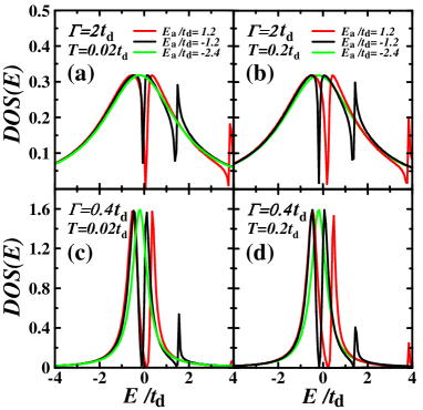
Figure 3: Density of states Eq.(8) for a strong coupling ($t_{C}/t_{d}=5$) in case I ($U_{d}=0$). (a) $T/t_{d}=0.02$ and (b) $T/t_{d}=0.2$ for a fast detector ($\Gamma/t_{d}=2$). (c) $T/t_{d}=0.02$ and (d)$T/t_{d}=0.2$ for a slow detector ($\Gamma/t_{d}=0.4$). $E_{d}=-0.2t_{d}$.$E_{F}=0$.

Figure 4: Mean field values as a function of $E_{a}(=E_{b})$: solutions of the self-consistent equations in case I. (a) fast detector. (b) slow detector. $T=0.02t_{d}$. $E_{d}=-0.2t_{d}$. $t_{d}=0.05$. $E_{F}=0$.

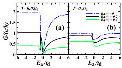
Figure 5: Conductance $G$ as a function of $E_{a}(=E_{b})$ for a weak coupling ($t_{C}/t_{d}=1$) in case I ($U_{d}=0$). (a) $T/t_{d}=0.02$ and (b)$T/t_{d}=0.2$ for a slow detector ($\Gamma/t_{d}=0.4$). Figure (a) shows that the dip structure is modulated for a slow detector when energy level $E_{d}$ is changed. $E_{F}=0$.

III.1 Case I: $U_{d}=0$

Figure 2 shows a conductance $G$ for strongly coupled two-level system ($t_{C}/t_{d}=5$) in case I. For a fast detector with $\Gamma/t_{d}=2$ (Fig. 2(a) and (b)), clear Fano dip can be seen in both low temperature ($T/t_{d}=0.02$) and high temperature ($T/t_{d}=0.2$). However, we cannot see the effect of the change caused by the bonding-antibonding state, even if we change $E_{d}$. When $\Gamma$ is reduced as shown in Fig.2 (c), we can see that the Fano dip is changed from a simple dip form to an asymmetric form at low temperature. The modulation of the structure in the $E_{d}<0$ region is considered to be an effect of the bonding-antibonding oscillation in the two-level system. These behaviors can be understood from DOS, which is derived from $\rho_{d}(\omega)=-{\rm Im}G_{dd}^{r}(\omega)/\pi$ :

$$\rho_{d}(\omega)=\frac{(\Gamma/\pi)D_{ab}^{2}}{\tilde{t}_{d}^{4}(\omega-\tilde{E}_{a})^{2}-2\tilde{t}_{d}^{2}(\omega-\tilde{E}_{d})(\omega-\tilde{E}_{a})D_{ab}+D_{ab}^{2}|B_{r}|^{2}}.$$ (8)

Instead of a single dip in the numerator in a T-shaped QDsWu , $D_{ab}$ in the numerator of Eq.(8) indicates double dips, that comes from bonding-antibonding state of side-QDs. Figure 3 shows four DOSs, which are displayed corresponding to Fig.2. We can see that there is a single peak for $E_{a}/t_{d}=-2.4$, closely distributed three peaks for $E_{a}/t_{d}=-1.2$, and separated three peaks for $E_{a}/t_{d}=1.2$. By comparing Figs. 3(a) and (c) with Figs. 3(b) and (d), respectively, we can see that temperature dependence on the shape of DOS is weak. Temperature slightly shifts the peak position. In contrast, $\Gamma$ dependence is large, similar to a Breit-Wigner function. The DOS of the slow detector (Fig. 3 (c)(d)) is sharper than that of the fast detector (Fig. 3 (a)(b)). $\Gamma$ mainly determines the width and the maximum value similar to T-shaped QD system. Because Eq.(7) is expressed as $G=-(2e/\hbar)\int d\omega\rho_{d}(\omega)z_{d}\Gamma_{R}\Gamma_{L}/(\Gamma_{R}+\Gamma_{L})\partial f_{L}(\omega)/\partial\omega$, conductance reflects an energy region $\pm T$ around $E_{F}$ in DOS. From $\partial f_{L}(\omega)/\partial\omega\rightarrow\delta(\omega)$ when $T\rightarrow 0$, at low temperature, conductance can detect the change of closely distributed three peaks in the DOS if those peaks are sufficiently sharp such as a slow detector. On the other hand, the present results show that the peak structure for a fast detector is not sufficiently sharp to detect the three peaks. At higher temperature, conductance integrates peak structures in DOS, resulting in the single-dip structures shown in Fig.2 (b) and (d). These are reasons of higher sensitivity of the slow detector at low temperature.

Figure  4 also shows the difference between a slow detector and a fast detector. Oscillations of mean field values for a fast detector (Fig.4 (a) ) are weaker than those for a slow detector (Fig.4 (b)) at $E_{a}<0$.

Figure 5 shows the case of weak coupling ($t_{C}/t_{d}=1$) in a slow detector. Fano dip modulation exists at lower temperature, but is smaller than that of Figure 2(c). At the higher temperature region of $T=0.2t_{d}$, we can observe a small and calm dip structure for both fast and slow detectors.

III.2 Case II: $U_{d}=\infty$

In this case, full self-consistent equations are applied so that the total number of electrons in QD $d$ is less than one, and we have to solve the six self-consistent equations from Eq.(2) to Eq.(6). Without QD $a$ and QD $b$, a Kondo peak is expected. In the case of T-shaped QDs, the Fano dip appears in the middle of Kondo peak conductanceTanaka . In the present case, the two energy levels in the side-QDs couple with the Kondo peak and produces the complicated conductance structure shown in Fig.6. Here, overall structure of $G$ does not change even in the region of $E_{d}<0$.

Figure 6: Conductance $G$ as a function of an energy level of the two-level system $E_{a}(=E_{b})$ for a strong coupling ($t_{C}/t_{d}=5$) in case II ($U_{d}=\infty$). (a) $\Gamma/t_{d}=2$ and (b)$\Gamma/t_{d}=0.4$. $E_{d}=E_{F}=0$.

IV Discussion

As noted in the introduction, the present model can be applied to several situations. If we look at QD $a$ as an extra trap site for the T-shaped QD system composed of QD $b$ and QD $d$ with both electrodes, the present calculation shows that a simple dip structure is most likely to be observed, and when the extra trap site is strongly coupled to the side QD $b$ and the energy level of QD $d$ is sufficiently low, the modulation of Fano dip could be observed. Experimentally, this would happen because it is not easy to exclude all trap sites from the QD system due to the difficulty of nanofabricationGores . The present calculations also indicate that when there are many additional trap sites, the Fano dip structure would be modulated further.

To construct a charge qubittana0 ; tanahu in the present case, the total number of electrons in QD $a$ and QD $b$ should be one. However, in the present setup, we only apply less than one electron in each QD. Thus, we need more restriction to hold one electron through the QD $a$ and QD $b$, for example, by introducing an exchange interaction such as that discussed in Ref.Lopez .

Although SBMFT is believed to be valid in previous works for one or two QDs, it has not yet been proved that this approximation is valid for many QD systems in the context of the Fano-Kondo effect. The effect of fluctuations around mean fields should be investigated in the near future.

V Conclusion

We have studied the transport properties of a triple QD system, in particular, emphasizing the Fano-Kondo effect through two-level system. We have used slave-boson mean field theory to describe quantum interference between electrons in discrete energy levels and free electrons in electrodes. We found that the Fano dip structure is modulated from simple dip to clear asymmetric form, when the coupling strength between the QDs in two-level system is large, using a slow detector without on-site Coulomb interaction in the detector QD. We also found that the Fano dip is strongly changed by Kondo resonance peak when there is an infinite Coulomb interaction in the detector QD.

Appendix A Green’s functions

Green’s functions are obtained based on equations of motion for the time ordered Green’s functions. Fourier-transferred diagonal Green’s functions for QDs are given as $G_{aa}^{r}(\omega)=[(\omega-\tilde{E}_{b})B_{r}-|\tilde{t}_{d}|^{2}]/B_{00}$ and $G_{bb}^{r}(\omega)=[(\omega-\tilde{E}_{a})B_{r}]/B_{00}$ other than $G_{dd}^{r}(\omega)$ expressed in the main text. We also have off-diagonal Green’s function by using relations $(\omega-\tilde{E}_{a})G_{ab}(\omega)=\tilde{t}_{C}G_{bb}(\omega)$ and $(\omega-\tilde{E}_{b}-|\tilde{t}_{d}|^{2}/(\omega-\tilde{E}_{a}))G_{ab}(\omega)=\tilde{t}_{d}G_{dd}(\omega)$. $G_{dk_{\alpha}}(\omega)$ and $G_{k_{\alpha}k_{\alpha}^{\prime}}(\omega)$($\alpha=L,R$) are obtained by $\{\omega-\tilde{E}_{d}-\Sigma_{b}-|\tilde{t}_{d}|^{2}/[\omega-\tilde{E}_{b}-|\tilde{t}_{d}|^{2}/(\omega-\tilde{E}_{a})]\}G_{dk_{\alpha}}(\omega)=V_{\alpha}/(\omega-E_{k_{\alpha}})$ and $(\omega-E_{k_{\alpha}})G_{k_{\alpha}k_{\alpha}^{\prime}}(\omega)=\delta_{k_{\alpha}k_{\alpha}^{\prime}}+V_{\alpha}G_{dk_{\alpha}}(\omega)$, with $\Sigma_{b}\equiv\sum_{\alpha}\sum_{k_{\alpha}}|V_{\alpha}|^{2}/(\omega-E_{k_{\alpha}})$. After applying analytic continuation rules, we obtain lesser Green’s functions in the current formula in the main text.

References

- (1) W. G. van der Wiel, S. De Franceschi, T. Fujisawa, J. M. Elzerman, S. Tarucha, and L. P. Kouwenhoven, Science 289 2105 (2000).
- (2) J. Göres, D. Goldhaber-Gordon, S. Heemeyer, and M. A. Kastner, H. Shtrikman, D. Mahalu, and U. Meirav, Phys. Rev. B62, 2188 (2000).
- (3) M. Sato, H. Aikawa, K. Kobayashi, S. Katsumoto, and Y. Iye, Phys. Rev. Lett. 95, 066801 (2005); K. Kobayashi, H. Aikawa, A. Sano, S. Katsumoto, and Y. Iye, Phys. Rev. 70, 035319 (2004).
- (4) K. Kang, S. Y. Cho, J. J. Kim and S. C. Shin, Phys. Rev. B 63, 113304 (2001).
- (5) A. A. Aligia and C. R. Proetto, Phys. Rev. B 65, 165305 (2002).
- (6) B. H. Wu, J. C. Cao and K. H. Ahn, Phys. Rev. B72, 165313 (2005).
- (7) A. D. Güclü, Q. F. Sun and H. Guo, Phys. Rev. B68, 245323 (2003).
- (8) Y. Tanaka and N. Kawakami, Phys. Rev. B72, 085304 (2005).
- (9) T. Tanamoto, Phys. Rev. A61, 022305 (2000), ibid,64 062306 (2001).
- (10) H. S. Goan, G. J. Milburn, H. M. Wiseman and H. B. Sun, Phys. Rev. B 63, 125326 (2001).
- (11) A. N. Korotkov, Phys. Rev. B 63, 115403 (2001).
- (12) T. Tanamoto and X. Hu, Phys. Rev. B69, 115301 (2004).
- (13) T. Gilad and S.A. Gurvitz, Phys. Rev. Lett. 97, 116806 (2006).
- (14) A. W. Rushforth, C. G. Smith, I. Farrer, D. A. Ritchie, G. A. C. Jones, D. Anderson, and M. Pepper, Phys. Rev. B 73, 081305(R) (2006).
- (15) S. Sasaki, S. Kang, K. Kitagawa, M. Yamaguchi, S. Miyashita, T. Maruyama, H. Tamura, T. Akazaki, Y. Hirayama and H. Takayanagi, Phys. Rev. B 73, 161303(R) (2006); H. Tamura and L. Glazman, Phys. Rev. B 72, 121308(R) (2005).
- (16) D M. Newns and N. Read, Adv. Phys. 36, 799 (1987); P. Coleman, Phys. Rev. B 35, 5072 (1987).
- (17) R. López, R. Aguado, and G. Platero, Phys. Rev. Lett. 89, 136802 (2002); T. Aono and M. Eto, Phys. Rev. B63, 125327 (2001).
- (18) C. A. Büsser, A. Moreo and E. Dagotto, Phys. Rev. 70, 035402 (2004); Z.-T. Jiang, Q.-F. Sun and Y. Wang, Phys. Rev. B72, 045332 (2005); R. Zitko, J. Bonca, A. Ramsak and T. Rejec, Phys. Rev. 73, 153307 (2006).