Multicriticality of the $(2+1)$-dimensional gonihedric model: A realization of the $(d,m)=(3,2)$ Lifshitz point

Abstract

Multicriticality of the gonihedric model in $2+1$ dimensions is investigated numerically. The gonihedric model is a fully frustrated Ising magnet with the finely tuned plaquette-type (four-body and plaquette-diagonal) interactions, which cancel out the domain-wall surface tension. Because the quantum-mechanical fluctuation along the imaginary-time direction is simply ferromagnetic, the criticality of the $(2+1)$-dimensional gonihedric model should be an anisotropic one; that is, the respective critical indices of real-space ($\perp$) and imaginary-time ($\parallel$) sectors do not coincide. Extending the parameter space to control the domain-wall surface tension, we analyze the criticality in terms of the crossover (multicritical) scaling theory. By means of the numerical diagonalization for the clusters with $N\leq 28$ spins, we obtained the correlation-length critical indices $(\nu_{\perp},\nu_{\parallel})=(0.45(10),1.04(27))$, and the crossover exponent $\phi=0.7(2)$. Our results are comparable to $(\nu_{\perp},\nu_{\parallel})=(0.482,1.230)$, and $\phi=0.688$ obtained by Diehl and Shpot for the $(d,m)=(3,2)$ Lifshitz point with the $\epsilon$-expansion method up to O$(\epsilon^{2})$.

I Introduction

Recently, a thorough investigation of the Lifshitz point was made by Diehl and Shpot with the $\epsilon$-expansion method up to O$(\epsilon^{2})$ Diehl00 ; Shpot01 ; see also Refs. Diehl03 ; Leite03a ; Leite03b ; Hornreich75 ; Mergulhao98 ; Mergulhao99 . The field theory for the Lifshitz point has an anisotropic dispersion like $\omega({\bf k})=\frac{1}{2}\sum_{i=1}^{m}k_{i}^{4}+\frac{1}{2}\sum_{i=m+1}^{d}k_{i}^{2}$, preventing us from going beyond order O$(\epsilon^{2})$. Reflecting this anisotropy, the critical indices within the subspaces, $i=1,2,\dots,m$ ($\perp$) and $i=m+1,m+2,\dots,d$ ($\parallel$), are no longer identical. In Ref. Shpot01 , the critical indices within each subspace are tabulated systematically for the generic values of $(d,m)$.

Such an anisotropic criticality is realized by the $d$-dimensional Ising model fully-frustrated within the $m$-dimensional subspace. The problem is that a naive computer simulation for the equilateral cluster does not yield adequate finite-size scaling. Rather, one has to adjust the shape of the cluster (that is, the system sizes of each subspace $L_{\parallel,\perp}$) so as to fix the following scaled ratio to a constant value;

$$L_{\perp}^{z}/L_{\parallel}=const.$$ (1)

Here, the index $z$ denotes the dynamical critical exponent, which characterizes the anisotropy. The significant point is that the exponent $z$ itself is an unknown parameter, and it has to be determined through some preliminary analyses. After that, one is able to perform large-scale simulations. So far, the case of $(d,m)=(3,1)$, namely, the axial-next-nearest-neighbor-Ising model, has been studied extensively by means of the Monte Carlo method Selke78 ; Kaski85 ; Pleimling01 . The simulation results are in agreement with the above-mentioned field-theoretical considerations as well as the series-expansion results Oitmaa85 ; Mo91 .

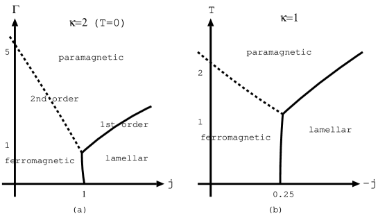
Figure 1: (a) A schematic drawing of the ground-state phase diagram of the $(2+1)$-dimensional gonihedric model, Eq. (2), with the self-avoidance parameter $\kappa=2$. We aim to investigate the multicritical point at $j=1$. (b) As a comparison, we present the phase diagram of the $d=3$ (classical) gonihedric model, Eq. (4), with $\kappa=1$ Cirillo97b ; Nishiyama04 ; here, the parameter $T$ denotes the temperature. The phase diagram is essentially the same as that of the quantum-mechanical model; the discrepancy $j\leftrightarrow-j$ is due to the difference of parameterization.

In this paper, we consider the case of $(d,m)=(3,2)$. For that purpose, we investigate the ground-state phase transition of the gonihedric model in $2+1$ dimensions. The gonihedric model is a fully frustrated Ising magnet with the finely tuned plaquette-type (four-body and plaquette-diagonal) interactions, for which the domain-wall surface tension vanishes; so far, the classical version has been studied in detail Savvidy94 ; Ambartzumian92 ; Cirillo97b ; Koutsoumbas02 ; Espriu97 . Making a contrast to the frustrated magnetism within the real space ($\perp$), the quantum fluctuation along the imaginary-time direction ($\parallel$) is simply ferromagnetic, and the ground-state criticality should be an anisotropic one. In Fig. 1 (a), we present a schematic phase diagram of the $(2+1)$-dimensional gonihedric model subjected to the transverse magnetic field $\Gamma$ and the frustration $j$; we explain the details in Sec. II. The multicritical point at $j=1$, where the magnetism is fully frustrated, is our main concern.

In order to simulate the $(2+1)$-dimensional gonihedric model, we utilize the numerical-diagonalization method. This approach may have the following advantages. First, we implemented Novotny’s method Novotny90 to represent the Hamiltonian-matrix elements; this method is readily applicable to the quantum-mechanical system as well Nishiyama07 . Owing to this method, we are able to treat an arbitrary number of spins $N=8,12,\dots,28$ constituting the $d=2$ cluster; note that conventionally, the number of spins is restricted within $N(=L^{2})=9,16,25,\dots$. Such an arbitrariness allows us to make a systematic finite-size scaling analysis. Second, the diagonalization method is free from the slowing-down problem; this problem becomes severe for such a frustrated magnetism, deteriorating the efficiency of the Monte Carlo sampling. Last, the constraint $L_{\perp}^{z}/L_{\parallel}\to 0$ [Eq. (1)] is always satisfied, because the system size along the imaginary-time direction is infinite $L_{\parallel}\to\infty$; note that the system size along the imaginary time corresponds to the inverse temperature $L_{\parallel}=1/T\to\infty$.

In fairness, it has to be mentioned that our research owes its basic idea to the following pioneering studies. First, an equivalence between the $(2+1)$-dimensional fully frustrated magnetism and the $(d,m)=(3,2)$ Lifshitz point was argued field-theoretically in Refs. Dutta97 ; Dutta98 . Second, in Ref. Pal90 , the biaxial-next-nearest-neighbor Ising model in $d=3$ was studied with the Monte Carlo method. It was reported that the Lifshitz (multicritical) point collapses at zero temperature. On the contrary, the gonihedric model has an extra tunable parameter $\kappa$. Setting $\kappa\geq 2$, we attain desirable multicriticality as depicted in Fig. 1 (a).

The rest of this paper is organized as follows. In Sec. II, we explain the $(2+1)$-dimensional gonihedric model. To elucidate the underlying physics, we make an overview of the classical gonihedric model in $d=3$. In Sec. III, we present the simulation results. The simulation scheme is explained in the Appendix. In Sec. IV, we present a summary and discussions.

II Quantum gonihedric model in $2+1$ dimensions: A realization of the $(d,m)=(3,2)$ Lifshitz point

In this section, we propose the $(2+1)$-dimensional gonihedric model as a realization of the $(d,m)=(3,2)$ Lifshitz point. To elucidate the underlying physics, we make an overview of the original (classical) gonihedric model in $d=3$.

II.1 Quantum gonihedric model in $d=2$

As mentioned in the Introduction, we propose the $(2+1)$-dimensional gonihedric model as a realization of the $(d,m)=(3,2)$ Lifshitz point. To be specific, we consider the Hamiltonian

$${\cal H}=-J_{1}\sum_{\langle ij\rangle}\sigma_{i}^{z}\sigma_{j}^{z}-J_{2}\sum_{\langle\langle ij\rangle\rangle}\sigma^{z}_{i}\sigma^{z}_{j}-J_{3}\sum_{[ijkl]}\sigma^{z}_{i}\sigma^{z}_{j}\sigma^{z}_{k}\sigma^{z}_{l}-\Gamma\sum_{i}\sigma^{x}_{i},$$ (2)

with the coupling constants $J_{1}=\kappa$, $J_{2}=-\kappa/2$, and $J_{3}=(1-\kappa)/2$. Here, the operators $\{\sigma^{\alpha}_{i}\}$ denote the Pauli matrices placed at the square-lattice points $i$. The summations $\sum_{\langle ij\rangle}$, $\sum_{\langle\langle ij\rangle\rangle}$, and $\sum_{[ijkl]}$ run over all possible nearest-neighbor, next-nearest-neighbor (plaquette diagonal), and plaquette-four-body spins, respectively. The transverse magnetic field $\Gamma$ controls the amount of quantum fluctuations. At a certain $\Gamma_{c}$, a ground-state phase transition may occur.

As mentioned above, the gonihedric model has finely tuned coupling constants $\{J_{i}\}$, which cancel out the domain-wall surface tension. Actually, the domain-wall energy of the gonihedric model (apart from the off-diagonal term $-\Gamma\sum_{i}\sigma^{x}_{i}$) admits a geometric representation $E=n_{2}+4\kappa n_{4}$ Savvidy94 . Here, $n_{2}$ denotes the number of points where two domain walls meet at a right angle (domain-wall undulation), and $n_{4}$ is the number of points where four domain walls meet at a right angle (self-intersection point). That is, the parameter $\kappa$ controls the self-avoidance of the domain walls with the bending elasticity unchanged. (Notably enough, the interfacial energy lacks the surface-tension term. Accordingly, the domain-wall undulations are promoted, giving rise to a peculiar type of criticality.) The gonihedric model has a tunable parameter $\kappa$ with the zero surface tension maintained. This redundancy is an advantage over other frustrated magnetisms such as the biaxial-next-nearest-neighbor Ising model. We survey the regime $\kappa\geq 2$, where we observed a clear indication of the Lifshitz-type criticality.

In this paper, we extend the above-mentioned parameterization space. That is, introducing a new controllable parameter $j$, we investigate the parameter space

$$J_{1}=\kappa,\ J_{2}=-\frac{\kappa j}{2},\ J_{3}=\frac{1-\kappa}{2}.$$ (3)

Note that at $j=1$, the parameter space, Eq. (3), reduces to the above-mentioned one (original gonihedric model). Owing to the extension, the magnetic domain wall now acquires a finite domain-wall surface tension $\propto 1-j$. In other worlds, in terms of this extended parameter space, we identify the Lifshitz point as a multicritical point; see the phase diagram in Fig. 1 (a). This viewpoint was proposed in Ref. Cirillo97b , where the authors investigate the criticality of the classical $d=3$ gonihedric model with the cluster-variation method. In the next section, we will overview the properties of the classical gonihedric model, which may be relevant to the present study.

II.2 Phase diagram of the classical gonihedric model: A brief overview

Let us make an overview of the past studies of the (classical) gonihedric model. The model was introduced by Savvidy and Wegner as a lattice-regularized version of the string field theory Savvidy94 ; Ambartzumian92 . However, recent developments dwell on the $d=3$ case, aiming at a potential applicability to microemulsions. The criticality should belong to the Lifshitz point with the index $(d,m)=(3,3)$, because the classical gonihedric model is isotropically frustrated. The $(d,m)=(3,3)$ criticality may be realized by the ternary mixture Dawson88 of water, oil and surfactant Huang81 ; Honorat84 ; Aschauer93 ; Seto96 ; actually, a crossover from the $d=3$-Ising universality to an exotic one was reported in Refs. Schwahn99 ; Stepanek02 .

We present a schematic phase diagram of the (classical) $d=3$ gonihedric model in Fig. 1 (b) Cirillo97b ; Nishiyama04 . The Hamiltonian of the classical $d=3$ gonihedric model is given by

$$H=-\sum_{\langle ij\rangle}S_{i}S_{j}-j\sum_{\langle\langle ij\rangle\rangle}S_{i}S_{j}-\frac{1-\kappa}{4\kappa}\sum_{[ijkl]}S_{i}S_{j}S_{k}S_{l}.$$ (4)

(The Ising-spin variables $\{S_{i}\}$ are placed at the $d=3$ lattice points.) We notice that the phase diagram resembles that of the quantum gonihedric model; the discrepancy as to $j\leftrightarrow-j$ is merely due to the difference of parameterization, and the subspace $-j=1/4$ corresponds to the fully-frustrated gonihedric model.

A few remarks on the phase diagram follow: First, the Lifshitz point at $-j=1/4$ is identified as an end-point of the critical branch ($-j<1/4$) belonging to the $d=3$-Ising universality. In fact, the multicritical (crossover) scaling theory applies successfully Cirillo97b ; Nishiyama04 to clarifying the nature of the Lifshitz point. (Direct numerical simulation at $-j=1/4$ appears to be rather problematic Hellmann93 .) We will accept this cross-over viewpoint as for the quantum gonihedric model. Second, in Refs. Koutsoumbas02 ; Espriu97 , it was reported that for small $\kappa<0.5$, the multicritical point becomes a discontinuous one, accompanied with pronounced hysteresis. In particular, at $\kappa=0$, the model reduces to the so-called $p$-spin model Shore91 , which is notorious for its slow relaxation to the thermal equilibrium (metastability). We found that a similar difficulty arises in the quantum gonihedric model. Hence, we devote ourselves to the large-$\kappa$ regime such as $\kappa\geq 2$, where we observed a clear indication of the Lifshitz-type criticality. Last, the phase boundary separating the lamellar and ferromagnetic phases is (almost) vertical. This feature ensures that the multicritical point is located at $-j=1/4$. The quantum gonihedric model possesses this property as shown in the next section. Actually, this is the most significant benefit of the parameterization scheme, Eq. (3).

III Numerical results

In this section, we present the numerical results. Our aim is to estimate the critical indices $(\nu_{\perp},\nu_{\parallel})$ and $\phi$. As mentioned in the Introduction, we utilize Novotny’s method to diagonalize the Hamiltonian (2) numerically. We explain the technical details in the Appendix. By means of this method, we simulated finite clusters with $N\leq 28$ spins. The linear dimension of the cluster $L$ is given by the formula

$$L=\sqrt{N},$$ (5)

because the $N$ spins constitute a $d=2$ cluster.

III.1 Finite-size scaling of the critical branch: $d=3$-Ising universality

In this section, we survey the critical branch $j<1$; see Fig. 1 (a). We show that the criticality belongs to the ordinary $d=3$-Ising universality class. This finding provides a foundation for the subsequent analyses with the crossover-scaling theory.

In Fig. 2, we plot the Roomany-Wyld approximate beta function Roomany80

$$\beta^{RW}_{N}(\Gamma)=\frac{1+\ln(\Delta E_{N}(\Gamma)/\Delta E_{N-4}(\Gamma))/\ln(\sqrt{N}/\sqrt{N-4})}{\sqrt{\partial_{\Gamma}\Delta E_{N}(\Gamma)\partial_{\Gamma}\Delta E_{N-4}(\Gamma)/\Delta E_{N}(\Gamma)/\Delta E_{N-4}(\Gamma)}},$$ (6)

with the excitation energy gap $\Delta E_{N}(\Gamma)$ for the system size $N$. Here, we fixed the self-avoidance parameter $\kappa=2$, and varied the frustration as $j=-1.2$, $-0.8$, $-0.4$, $0$, and $0.4$. The zero point of the beta function indicates the location of the critical point $\Gamma_{c}(j)$. Basically, the critical branch depicted in Fig. 1 (a) follows from this analysis; afterward, we determine the critical point $\Gamma_{c}$ more precisely.

The slope of the beta function at $\Gamma=\Gamma_{c}$ yields an estimate for the inverse of the correlation-length critical exponent, $1/\nu$. In Fig. 2, as a reference, we presented a slope (dotted line) $1/\nu=1.5868$ Deng03 corresponding to the $d=3$-Ising universality class. We see that the criticality is maintained in the $d=3$-Ising universality class for a wide range of $j$. Actually, we obtained $1/\nu=1.55$, $1.54$, $1.51$, $1.46$, and $1.39$ for $j=-1.2$, $-0.8$, $-0.4$, $0$, and $0.4$, respectively. These results demonstrate that the critical branch belongs to the $d=3$-Ising universality class. It would be noteworthy that the shape of the beta function becomes distorted as $j\to 1$. That is, the regime exhibiting the slope $1/\nu$ shrinks gradually as $j\to 1$, indicating that a new type of criticality emerges at the multicritical point $j=1$. Actually, we consider this crossover behavior rather in detail in the following sections.

In Fig. 3, we present the approximate critical point $\Gamma_{c}(L_{1},L_{2})$ for $[2/(L_{1}+L_{2})]^{1/\nu+\omega}$ Binder81 with $\kappa=2$, $j=-0.4$, and $8\leq N_{1}<N_{2}\leq 28$ ($L_{1,2}=\sqrt{N_{1,2}}$); here, we used the corrections-to-scaling exponent $\omega=0.821$ and the exponent $\nu=1.5868^{-1}$ reported in Ref. Deng03 . The approximate critical point $\Gamma_{c}(L_{1},L_{2})$ is determined by the zero point of the beta function. That is, it satisfies the equation

$$\sqrt{N_{1}}\Delta E_{N_{1}}(\Gamma_{c}(L_{1},L_{2}))=\sqrt{N_{2}}\Delta E_{N_{2}}(\Gamma_{c}(L_{1},L_{2})).$$ (7)

From the least-squares fit to the data in Fig. 3, we obtained the critical point $\Gamma_{c}=7.073(55)$ in the thermodynamic limit $L\to\infty$. We make use of $\Gamma_{c}$ in the following scaling analyses.

III.2 End-point singularity of the critical amplitude

The above analysis indicates that the multicriticality at $j=1$ is merely an end-point singularity of the ordinary $d=3$-Ising critical branch. That is, the crossover-scaling theory should apply to clarifying the nature of the multicritical point.

In this section, we consider the singularity of the critical amplitude of $\Delta E$ beside the multicritical point. The amplitude $G^{\pm}$ is defined by the relation

$$\Delta E\approx G^{\pm}(j)|\Gamma-\Gamma_{c}(j)|^{\nu}.$$ (8)

The amplitude exhibits the singularity

$$G^{\pm}(\Delta)\sim\Delta^{(\nu_{\parallel}-\nu)/\phi},$$ (9)

with the crossover exponent $\phi$. (As mentioned in the Introduction, the exponent $\nu_{\parallel}$ denotes the critical index along the imaginary-time direction.) The variable $\Delta$ stands for the distance from the multicritical point

$$\Delta=1-j.$$ (10)

Here, we postulated that the multicritical point locates at $j=1$, and we justify this claim in Sec. III.4. The above formula is a straightforward consequence of the crossover-scaling hypothesis

$$\Delta E\approx|\Gamma-\Gamma_{c}|^{\nu_{\parallel}}f(\Delta/|\Gamma-\Gamma_{c}|^{\phi}).$$ (11)

Actually, this relation provides a definition of the crossover exponent $\phi$.

To begin with, we determine the critical amplitude $G^{+}$. In Fig. 4, we plot the scaled energy gap $(\Gamma-\Gamma_{c})L^{1/\nu}$-$\Delta E/|\Gamma-\Gamma_{c}|^{\nu}$ for $\kappa=2$, $j=-0.4$, and $N=8,12,\dots,28$. The critical point $\Gamma_{c}=7.073$ is determined in the above section, and likewise, we postulated the $d=3$-Ising universality class $1/\nu=1.5868$ Deng03 . The data collapse into a scaling-function curve. We again confirm that the phase transition belongs to the $d=3$-Ising universality class. From the limiting value of the high-$\Gamma$ side of the scaling function, we estimate the critical amplitude as $G^{+}=4.28(8)$; here, we read off the value around the scaling regime $(\Gamma-\Gamma_{c})L^{1/\nu}=15$, and accepted the data scatter among $N=20$, $24$ and $28$ as an error indicator.

Similarly, we determined $G^{+}$ for various values of $j$ and $\kappa=2$, 4, and 6. In Fig. 5, we plotted the amplitude $G^{+}$ for $\Delta(=1-j)$ with the logarithmic scale. [In the cases of $\kappa=2$, $4$, and $6$, we read off $G^{+}$ from the scaling plot at the scaling regime $(\Gamma-\Gamma_{c})L^{1/\nu}=15$, 40, and 60, respectively. In the case of $\kappa=2$, we omitted the data of $N=16$ for its rather insystematic behavior particularly for small $\Delta$.] In the plot, we also presented a slope (dotted line) of $G^{+}\propto\Delta^{0.6}$. We observe a signature of the power-law singularity with the exponent $(\nu_{\parallel}-\nu)/\phi\approx 0.6$ as $\Delta\to 0$. Hence, we confirm that the crossover behavior (9) is realized in the vicinity of the multicritical point. In fact, from $\nu=0.63020(12)$ Deng03 and the present results, Eqs. (19) and (16), obtained in Sec. III.3, we arrive at the slope

$$\frac{\nu_{\parallel}-\nu}{\phi}=0.59(42),$$ (12)

fairly consistent with the above observation. With use of $G^{+}$ calculated in this section, we crosscheck the validity of the critical indices obtained in the following section.

III.3 Finite-size-scaling analysis of $(\nu_{\perp},\nu_{\parallel})$ and $\phi$

In this section, we make an analysis of each critical exponent with use of the crossover scaling, Eq. (11).

First, we consider the Binder parameter

$$U=1-\frac{\langle M^{4}\rangle}{3\langle M^{2}\rangle^{2}},$$ (13)

with the magnetization $M=\sum_{i=1}^{N}\sigma^{z}_{i}$. [Note that the simulation was not done right at the Lifshitz point; we calculated the data in the vicinity of the Lifshitz point (crossover scaling). Hence, the ferromagnetic order parameter $M$ is still of use in the data analysis.] The symbol $\langle\dots\rangle$ denotes the expectation value at the ground state. According to the crossover-scaling theory, the Binder parameter obeys the formula

$$U=\tilde{U}((\Gamma-\Gamma_{c})L^{1/\nu_{\perp}},\Delta L^{\phi/\nu_{\perp}}).$$ (14)

(Here, we made use of the fact that the Binder parameter is scale-invariant at the critical point.) As noted in the Introduction, the index with the subscript $\perp$ denotes the critical exponent within the real space. In Fig. 6, we present the crossover-scaling plot, $(\Gamma-\Gamma_{c})L^{1/\nu_{\perp}}$-$U$, with $\kappa=2$ and $\Delta L^{\phi/\nu_{\perp}}=8$. Here, we set the scaling parameters $\nu_{\perp}=0.45$ and $\phi=0.7$, where we found the best data collapse. Surveying $\kappa=4$ and $6$ as well, we arrive at the estimates

$$\nu_{\perp}=0.45(10),$$ (15)

and

$$\phi=0.7(2).$$ (16)

Second, we consider the energy gap $\Delta E$. The energy gap obeys the crossover-scaling relation

$$\Delta E=L^{-z}g((\Gamma-\Gamma_{c})L^{1/\nu_{\perp}},\Delta L^{\phi/\nu_{\perp}}),$$ (17)

with the dynamical critical exponent $z$. In Fig. 7, we present the crossover-scaling plot, $(\Gamma-\Gamma_{c})L^{1/\nu_{\perp}}$-$L^{z}\Delta E$, with $\kappa=2$ and $\Delta L^{\phi/\nu_{\perp}}=8$. Here, we set $z=2.3$, and the other scaling parameters are the same as those of Fig. 6. Surveying $\kappa=4$ and $6$ as well, we estimate the critical index as

$$z=2.3(3).$$ (18)

Through $z=\nu_{\parallel}/\nu_{\perp}$, the above results lead to

$$\nu_{\parallel}=1.04(27).$$ (19)

Let us address a remark. As mentioned in the above section, the indices, Eqs. (16) and (19), are consistent with the end-point singularity of $G^{+}$, indicating the self-consistency of the present analyses.

III.4 Phase transition between the ferromagnetic and lamellar phases

The above analysis stems from the proposition that the multicritical point locates at $j=1$; in other words, the phase boundary separating the ferromagnetic and lamellar phases is (almost) vertical. In this section, we justify this proposition. (Actually, this feature was confirmed in the case of the classical $d=3$ gonihedric model Cirillo97b .)

In Fig. 8, we plot the ground-state energy per unit cell $E_{0}/N$ with the system sizes $N=8,12,\dots,28$ for $\kappa=2$ and $\Gamma=0.6$; namely, we surveyed the regime slightly below the multicritical point. We observe a distinct signature of the first-order phase transition around $j\approx 1$, where the slope of $E_{0}/N$ changes rather abruptly (level crossing). The transition point seems to converge into the regime $0.9\leq j_{c}\leq 1$ as $N\to\infty$. Noticeably enough, the transition point is close to $j=1$.

We argue this behavior more in detail: First, the data $E_{0}/N$ in $j<j_{c}$ (ferromagnetic phase) appear to reach the thermodynamic limit, whereas in $j>j_{c}$ (lamellar phase), the plots are still scattered insystematically. Possibly, the incommensurability of the lamellar-type structure (periodicity of the domain walls) causes such an irregularity. Surveying the cases of $\kappa=2$, $4$, and $6$, we found that the data of $N=8$, 16, and 24 are rather robust against this incommensurability effect. Hence, we conclude that the transition point locates within $0.9\leq j_{c}\leq 1$. Last, we found that such a slight deviation of $j_{c}$ from $j=1$ is negligible in the sense that the influence is less than the error margins. In other worlds, the parameterization, Eq. (3), is sensible to explore the multicriticality in terms of the cross-over scaling; this point was noted in the case of the classical gonihedric model Cirillo97b .

IV Summary and discussions

We investigated the criticality of the $(2+1)$-dimensional gonihedric model, Eq. (2), with the extended parameter space, Eq. (3). This extended parameter space allows us to survey the criticality in terms of the crossover-scaling theory; see Fig. 1 (a). We employed Novotny’s method to diagonalize the Hamiltonian. With use of this method, we treated an arbitrary (integral) number of spins $N=8,12,\dots,28$. Because the quantum-mechanical fluctuation along the imaginary time direction is ferromagnetic, the criticality of the quantum gonihedric model should be an anisotropic one accompanied with the dynamical critical exponent $z(=\nu_{\parallel}/\nu_{\perp})\neq 1$. Our estimates for the critical indices are $(\nu_{\perp},\nu_{\parallel})=(0.45(10),1.04(27))$ and $\phi=0.7(2)$. We also confirmed that the estimates are consistent with the end-point singularity of the critical amplitude $G^{+}$; see Fig. 5

As mentioned in the Introduction, Diehl and Shpot made an analysis of the Lifshitz point with the $\epsilon$-expansion method up to O$(\epsilon^{2})$. Their conclusions for $(d,m)=(3,2)$ are

$$(\nu_{\perp},\nu_{\parallel})=(0.387,0.795)\ and\ \phi=0.686.$$ (20)

They also provided the convergence-accelerated results with the $[1/1]$ Padé method;

$$(\nu_{\perp},\nu_{\parallel})=(0.482,1.230)\ and\ \phi=0.688.$$ (21)

Our simulation data support their claim.

Lastly, let us make a few comments on the advantages of the diagonalization approach. First, the numerical diagonalization is free from the slowing-problem problem, which deteriorates the efficiency of the Monte Carlo sampling for the frustrated magnetism. Second, we do not have to worry about the constraint (1). The constraint is always satisfied, because the system size along the imaginary-time direction is infinite. However, the diagonalization method suffers from the severe limitation as to the available system sizes. In this paper, we surmount this difficulty with the aide of Novotny’s method, which allows us to treat a variety of system sizes $N=8,12,\dots,28$ sufficient to manage systematic finite-size scaling.

Appendix A Construction of the Hamiltonian-matrix elements: Quantum Novotny’s method

In this Appendix, we explain the simulation scheme. As mentioned in the Introduction, we applied the Novotny method Novotny90 to diagonalizing the Hamiltonian (2). Novotny’s method allows us to construct the Hamiltonian-matrix elements systematically for the cluster with an arbitrary (integral) number of spins $N=8,12,\dots,28$; note that conventionally, the number of spins is restricted within $N(=L^{2})=9,16,25,\dots$. Originally, Novotny’s method was formulated for the classical Ising model (transfer-matrix formalism) Novotny90 . In Ref. Nishiyama07 , it was extended to adopt the quantum-mechanical interaction (Hamiltonian formalism). Here, we follow the notation of Ref. Nishiyama07 , and make a slight extension to incorporate the plaquette-type interactions; see Eq. (26).

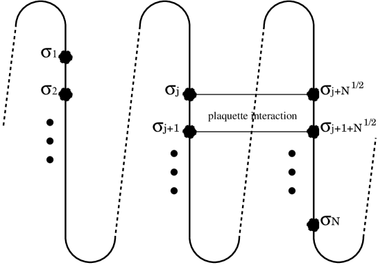
Figure 9: Construction of the spin cluster for the gonihedric model (2). As indicated above, the spins constitute a $d=1$-dimensional alignment $\{\sigma_{i}\}$ ($i=1,2,\dots,N$), and the dimensionality is lifted to $d=2$ by introducing the bridges (long-range interactions) over the ($N^{1/2}$)th-neighbor pairs.

Before we commence a detailed discussion, we explain the basic idea of Novotny’s method. In Fig. 9, we present a schematic drawing of a finite-size cluster for the $d=2$ gonihedric model, Eq. (2). As seen in the figure, the spins $\{\sigma_{i}\}$ ($i=1,2,\dots,N$) constitute a $d=1$-dimensional (zig-zag) structure. This feature is essential for us to construct the cluster with an arbitrary (integral) number of spins $N$. The dimensionality is lifted to $d=2$ by the long-range interactions over the $\sqrt{N}$th-neighbor distances; owing to the long-range interaction, the $N$ spins constitute a $\sqrt{N}\times\sqrt{N}$ rectangular network effectively. (The significant point is that the number $\sqrt{N}$ is not necessarily an integral nor rational number.)

Let us formulate the above idea explicitly. To begin with, we set up the Hilbert-space bases $\{|\sigma_{1},\sigma_{2},\dots,\sigma_{N}\rangle\}$ ($\sigma_{i}=\pm 1$) for the quantum spins $\{\sigma_{i}^{\alpha}\}$ ($i=1,2,\dots,N$). The bases diagonalize the operator $\sigma^{z}_{i}$; namely, the relation

$$\sigma_{j}^{z}|\{\sigma_{i}\}\rangle=\sigma_{j}|\{\sigma_{i}\}\rangle,$$ (22)

holds.

We decompose the Hamiltonian into two components

$${\cal H}={\cal H}^{(D)}(\{J_{i}\})+{\cal H}^{(O)}(\Gamma).$$ (23)

The component ${\cal H}^{(D)}(\{J_{i}\})$ describes the exchange interactions, depending on the coupling constants $\{J_{i}\}$. On the other hand, the component ${\cal H}^{(O)}(\Gamma)$ originates from the single-spin term, which depends on the transverse magnetic field $\Gamma$. The former component is a diagonal matrix, whereas the latter is off-diagonal.

First, we consider the diagonal component ${\cal H}^{(D)}$. We propose the following formula Nishiyama07

$${\cal H}^{(D)}=\frac{1}{2}(H(\sqrt{N})+H(-\sqrt{N})).$$ (24)

Here, the component $H(v)$ is a diagonal matrix, which describes the $v$th-neighbor interaction among the $N$-spin alignment. The diagonal elements are given by

$$H_{\{\sigma_{i}\},\{\sigma_{i}\}}(v)=\langle\{\sigma_{i}\}|H(v)|\{\sigma_{i}\}\rangle=\langle\{\sigma_{i}\}|TP^{v}|\{\sigma_{i}\}\rangle.$$ (25)

Here, the matrix $T$ denotes the plaquette-type interaction between the arrays $\{\sigma_{i}\}$ and $\{\tau_{i}\}$;

$$\langle\{\sigma_{i}\}|T|\{\tau_{i}\}\rangle=\sum_{k=1}^{N}\left(-\frac{J_{1}}{2}(\sigma_{k}\sigma_{k+1}+\tau_{k}\tau_{k+1}+\sigma_{k}\tau_{k}+\sigma_{k+1}\tau_{k+1})-J_{2}(\sigma_{k}\tau_{k+1}+\sigma_{k+1}\tau_{k})-J_{3}\sigma_{k}\sigma_{k+1}\tau_{k}\tau_{k+1}\right).$$ (26)

The operator $P$ denotes the translational operator, which satisfies $P|\{\sigma_{i}\}\rangle=|\{\sigma_{i+1}\}\rangle$; here, we imposed the periodic-boundary condition. Note that the operator insertion of $P^{v}$ in Eq. (25) introduces the long-range interaction over the $v$th-neighbor pairs. The denominator $2$ in Eqs. (24) and (26) compensates the duplicated sum.

Lastly, we consider the off-diagonal component ${\cal H}^{(O)}$. The matrix element is given by

$${\cal H}^{(O)}_{\{\sigma_{i}\},\{\tau_{i}\}}=\langle\{\sigma_{i}\}|{\cal H}^{(O)}|\{\tau_{i}\}\rangle.$$ (27)

The expression is quite standard, because the component ${\cal H}^{(O)}$ simply concerns the individual spins, and has nothing to do with the connectivity among them.

The above formulas complete our basis to simulate the Hamiltonian (2) numerically. The results are shown in Sec. III.

Figure 2: The beta function $\beta^{RW}_{28}(\Gamma)$ (6) is plotted for $\kappa=2$ and various $j$. The symbols, $+$, $\times$, $*$, $\Box$, and $\blacksquare$, denote the data for $j=0.4$, $0$, $-0.4$, $-0.8$, and $-1.2$, respectively. For a comparison, we presented a slope (dotted line) corresponding to the $d=3$-Ising universality class ($\nu=0.6294$ Deng03 ). We see that the criticality is maintained to be that of the $d=3$-Ising universality class for a wide range of $j$; see text for details.

Figure 3: The approximate critical point $\Gamma_{c}(L_{1},L_{2})$ is plotted for $[2/(L_{1}+L_{2})]^{1/\nu+\omega}$ with $8\leq N_{1}<N_{2}\leq 28$, $\kappa=2$, and $j=-0.4$; the corrections-to-scaling exponent $\omega=0.821$ and the exponent $1/\nu=1.5868$ are taken from Ref. Deng03 . The least-squares fit to these data yields $\Gamma_{c}=7.073(55)$ in the thermodynamic limit.

Figure 4: The scaling plot for the energy gap, $(\Gamma-\Gamma_{c})L^{1/\nu}$- $\Delta E/|\Gamma-\Gamma_{c}|^{\nu}$, is shown. The parameters are the same as those of Fig. 3. We postulated the $d=3$-Ising universality class $\nu=0.6302$ Deng03 . The symbols, $+$, $\times$, $*$, $\Box$, $\blacksquare$, and $\circ$, denote the system sizes of $N=8$, 12, 16, 20, 24, and 28, respectively. We confirm that the transition belongs to the $d=3$-Ising universality class. Furthermore, from the plateau in the high-$\Gamma$ side, we obtain an estimate for the critical amplitude $G^{+}=4.28(8)$; see text for details.

Figure 5: The correlation-length critical amplitude $G^{+}$ (9) is plotted for various $\Delta(=1-j)$ and $\kappa=2$, 4, and 6. The symbols $\times$, $\Box$, and $\circ$ denote the data for $\kappa=2$, 4, and 6, respectively. As a reference, we presented a slope (dotted line) of $G^{+}\propto\Delta^{0.6}$. The data indicate a power-law singularity, Eq. (9), with the exponent $(\nu_{\parallel}-\nu)/\phi\approx 0.6$; see text for details.

Figure 6: The crossover-scaling plot (14), $(\Gamma-\Gamma_{c})L^{1/\nu_{\perp}}$-$U$, for $\kappa=2$ and $\Delta L^{\phi/\nu_{\perp}}=8$ is shown. Here we set $\nu_{\perp}=0.45$ and $\phi=0.7$, for which we found the best data collapse. The symbols, $+$, $\times$, $*$, $\Box$, $\blacksquare$, and $\circ$, denote the system sizes of $N=8$, 12, 16, 20, 24, and 28, respectively.

Figure 7: The crossover-scaling plot (17), $(\Gamma-\Gamma_{c})L^{1/\nu_{\perp}}$-$L^{z}\Delta E$, is shown. Here, we set $z=2.3$, and the other scaling parameters are the same as those of Fig. 6. The symbols, $+$, $\times$, $*$, $\Box$, $\blacksquare$, and $\circ$, denote the system sizes of $N=8$, 12, 16, 20, 24, and 28, respectively.

Figure 8: The ground-state energy per unit cell $E_{0}/N$ is plotted for $\kappa=2$ and $\Gamma=0.6$. The symbols, $+$, $\times$, $*$, $\Box$, $\blacksquare$, and $\circ$, denote the system sizes of $N=8$, 12, 16, 20, 24, and 28, respectively. There occurs a transition separating the ferromagnetic and lamellar phases. The transition point seems to converge into the regime $0.9\leq j_{c}\leq 1$ as $N\to\infty$; see text for details,

References

- (1) H. W. Diehl and M. Shpot, Phys. Rev. B 62, 12338 (2000).
- (2) M. Shpot and H. W. Diehl, Nucl. Phys. B 612, 340 (2001).
- (3) H. W. Diehl and M. Shpot, Phys. Rev. B 68, 066401 (2003).
- (4) M. M. Leite, Phys. Rev. B 67, 104415 (2003).
- (5) M. M. Leite, Phys. Rev. B 68, 066402 (2003).
- (6) R. M. Hornreich, M. Luban, and S. Shtrikman, Phys. Rev. Lett. 35, 1678 (1975).
- (7) C. Mergulhão, Jr and C. E. I. Carneiro, Phys. Rev. B 58, 6047 (1998).
- (8) C. Mergulhão, Jr and C. E. I. Carneiro, Phys. Rev. B 59, 13954 (1999).
- (9) W. Selke, Z. Phys. B 29, 133 (1978).
- (10) K. Kaski and W. Selke, Phys. Rev. B 31, 3128 (1985).
- (11) M. Pleimling and M. Henkel, Phys. Rev. Lett. 87, 125702 (2001).
- (12) J. Oitmaa, J. Phys. A: Math. Gen. 18, 365 (1985).
- (13) Z. Mo and M. Ferer, Phys. Rev. B 43, 10890 (1991).
- (14) G.K. Savvidy and F.J. Wegner, Nucl. Phys. B 413, 605 (1994).
- (15) R.V. Ambartzumian, G.S. Sukiasian, G.K. Savvidy, and K.G. Savvidy, Phys. Lett. B 275, 99 (1992).
- (16) E.N.M. Cirillo, G. Gonnella, and A Pelizzola, Phys. Rev. E 55, R17 (1997).
- (17) G. Koutsoumbas and G.K. Savvidy, Mod. Phys. Lett. A 17, (2002) 751.
- (18) D. Espriu, M. Baig, D.A. Johnston, and Ranasinghe P.K.C. Malmini, J. Phys. A: Math. Gen. 30, 405 (1997).
- (19) M.A. Novotny, J. Appl. Phys. 67, 5448 (1990).
- (20) Y. Nishiyama, Phys. Rev. E 75, 011106 (2007).
- (21) A. Dutta, B. K. Chakrabarti, and J. K. Bhattacharjee, Phys. Rev. B 55, 5619 (1997).
- (22) A. Dutta, J. K. Bhattacharjee, and B. K. Chakrabarti, Eur. Phys. J. B 3, 97 (1998).
- (23) B. Pal and S. Dasgupta, Z. Phys. B 78, 489 (1990).
- (24) K.A. Dawson, M.D. Lipkin, and B. Widom, J. Chem. Phys. 88, 5149 (1988).
- (25) J. S. Huang and M. W. Kim, Phys. Rev. Lett. 47, 1462 (1981).
- (26) P. Honorat, D. Roux, and A. M. Bellocq, J. Phys. (Paris) Lett. 45, L-961 (1984).
- (27) R. Aschauer and D. Beysens, Phys. Rev. E 47, 1850 (1993).
- (28) H. Seto, D Schwahn, M Nagao, E Yokoi, S Komura, M Imai, and K Mortensen, Phys. Rev. E 54, 629 (1996).
- (29) D. Schwahn, K. Mortensen, H. Frielinghaus, and K. Almdal, Phys. Rev. Lett. 82, 5056 (1999).
- (30) P. Štěpánek, T. L. Morkved, K. Krishnan, T. P. Lodge, and F. S. Bates, Physica A 314, 411 (2002).
- (31) Y. Nishiyama, Phys. Rev. E 70, 026120 (2004).
- (32) R.K. Hellmann, A.M. Ferrenberg, D.P. Landau, and R.W. Gerling, Computer Simulation Studies in Condensed-Matter Physics IV, edited by D.P. Landau, K.K. Mon, and H.-B. Schüttler (Springer-Verlag, Berlin, 1993).
- (33) J.D. Shore and J.P. Sethna, Phys. Rev. B 43, 3782 (1991).
- (34) H.H. Roomany and H.W. Wyld, Phys. Rev. D 21, 3341 (1980).
- (35) Y. Deng and H.W.J. Blöte, Phys. Rev. E 68, 036125 (2003).
- (36) K. Binder, Z. Phys. B: Condens. Matter 43, 119 (1981).