Statistics of an Unstable Barotropic Jet from a Cumulant Expansion

Abstract

Low-order equal-time statistics of a barotropic flow on a rotating sphere are investigated. The flow is driven by linear relaxation toward an unstable zonal jet. For relatively short relaxation times, the flow is dominated by critical-layer waves. For sufficiently long relaxation times, the flow is turbulent. Statistics obtained from a second-order cumulant expansion are compared to those accumulated in direct numerical simulations, revealing the strengths and limitations of the expansion for different relaxation times.

1 Introduction

Many geophysical flows are subject to the effects of planetary rotation and to forcing and dissipation on large scales. For example, the kinetic energy of atmospheric macroturbulence is generated by baroclinic instability and is then partially transferred to mean flows, whose energy dissipation can often be represented by large-scale dissipation. Statistically steady states of such flows can exhibit regions of strong mixing that are clearly separated from regions of weak or no mixing, implying that the mixing is non-ergodic in the sense that flow states are not phase-space filling on phase space surfaces of constant inviscid invariants such as energy and enstrophy (Shepherd 1987). As a consequence, concepts from equilibrium statistical mechanics, which rely on ergodicity assumptions and can account for the statistics of two-dimensional flows in the absence of large-scale forcing and dissipation (e.g., Miller 1990; Robert and Sommeria 1991; Turkington et al. 2001; Majda and Wang 2006), generally cannot be used in developing statistical closures for such flows.

In this paper, we investigate the inhomogeneous statistics of what may be the simplest flow subject to rotation, large-scale forcing, and dissipation that exhibits mixing and no-mixing regions in statistically steady states: barotropic flow on a rotating sphere driven by linear relaxation toward an unstable zonal jet. Depending on a single control parameter, the relaxation time, this prototype flow exhibits behavior in the mixing region near the jet center that ranges from critical-layer waves at short relaxation times to turbulence at sufficiently long relaxation times. This permits systematic tests of non-equilibrium statistical closures in flow regimes ranging from weakly to strongly nonlinear.

We study a non-equilibrium statistical closure based on a second-order cumulant expansion (CE) of the equal-time statistics of the flow. The CE is closed by constraining the third and higher cumulants to vanish, and the resulting second-order cumulant equations are solved numerically. The CE is weakly nonlinear in that nonlinear eddy–eddy interactions are assumed to vanish. We show that for short relaxation times, the CE accurately reproduces equal-time statistics obtained by direct numerical simulation (DNS). For long relaxation times, the CE does not quantitatively reproduce the DNS statistics but still provides information, for example, on the location of the boundary between the mixing and the no-mixing region—information that local closures (e.g., diffusive closures) do not easily provide.

Section 2 introduces the equations of motion for the flow and discusses their symmetries and conservation laws. Section 3 describes the DNS, including the accumulation of low-order equal-time statistics during the course of the simulation. The CE and its associated closure approximation are outlined in section 4. Section 5 compares DNS and CE. Implications of the results are discussed in section 6.

2 Barotropic jet on a rotating sphere

a Equations of motion

We study forced-dissipative barotropic flow on a sphere of radius $a$ rotating with angular velocity $\Omega$. Though not crucial for this paper, we prefer to work on the sphere and not in the $\beta$-plane approximation, as the sphere can support interesting phenomena not found on the plane (e.g., Cho and Polvani 1996). The absolute vorticity $q$ is given by

$$q = \zeta+f$$ (1)

$$= \nabla^{2}\psi+f$$

where $\zeta$ is the relative vorticity, $\psi$ is the stream function, $\nabla^{2}$ is the Laplacian on the sphere, and

$$f(\phi)=2\Omega\sin\phi$$ (2)

is the Coriolis parameter, which varies with latitude $\phi$. The time evolution of the absolute vorticity is governed by the equation of motion (EOM)

$${{\partial q}\over{\partial t}}+J[\psi,q]=\frac{q_{\rm jet}-q}{\tau},$$ (3)

where

$$J[\psi,q]\equiv\frac{1}{a^{2}\cos(\phi)}\left(\frac{\partial\psi}{\partial\lambda}\frac{\partial q}{\partial\phi}-\frac{\partial\psi}{\partial\phi}\frac{\partial q}{\partial\lambda}\right)$$ (4)

is the Jacobian on the sphere and $\lambda$ is longitude. Forcing and dissipation are represented by the term on the right-hand-side of Eq. (3), which linearly relaxes the absolute vorticity $q$ to the absolute vorticity $q_{\rm jet}$ of a zonal jet on a relaxation time $\tau$.

The zonal jet is symmetric about the equator and is characterized by constant relative vorticities $\pm\Gamma$ on the flanks far away from the apex and by a rounding width $\Delta\phi$ of the apex,

$$q_{\rm jet}(\phi)=f(\phi)-\Gamma\tanh\left(\frac{\phi}{\Delta\phi}\right)\ .$$ (5)

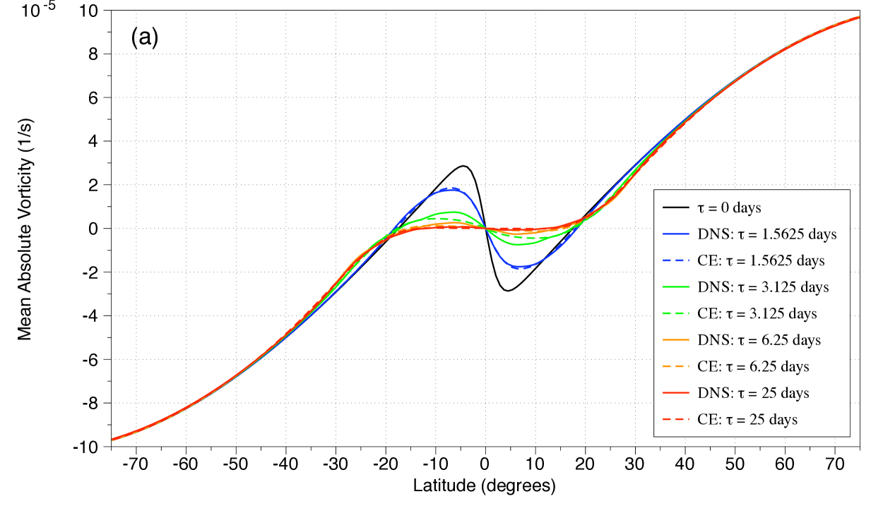
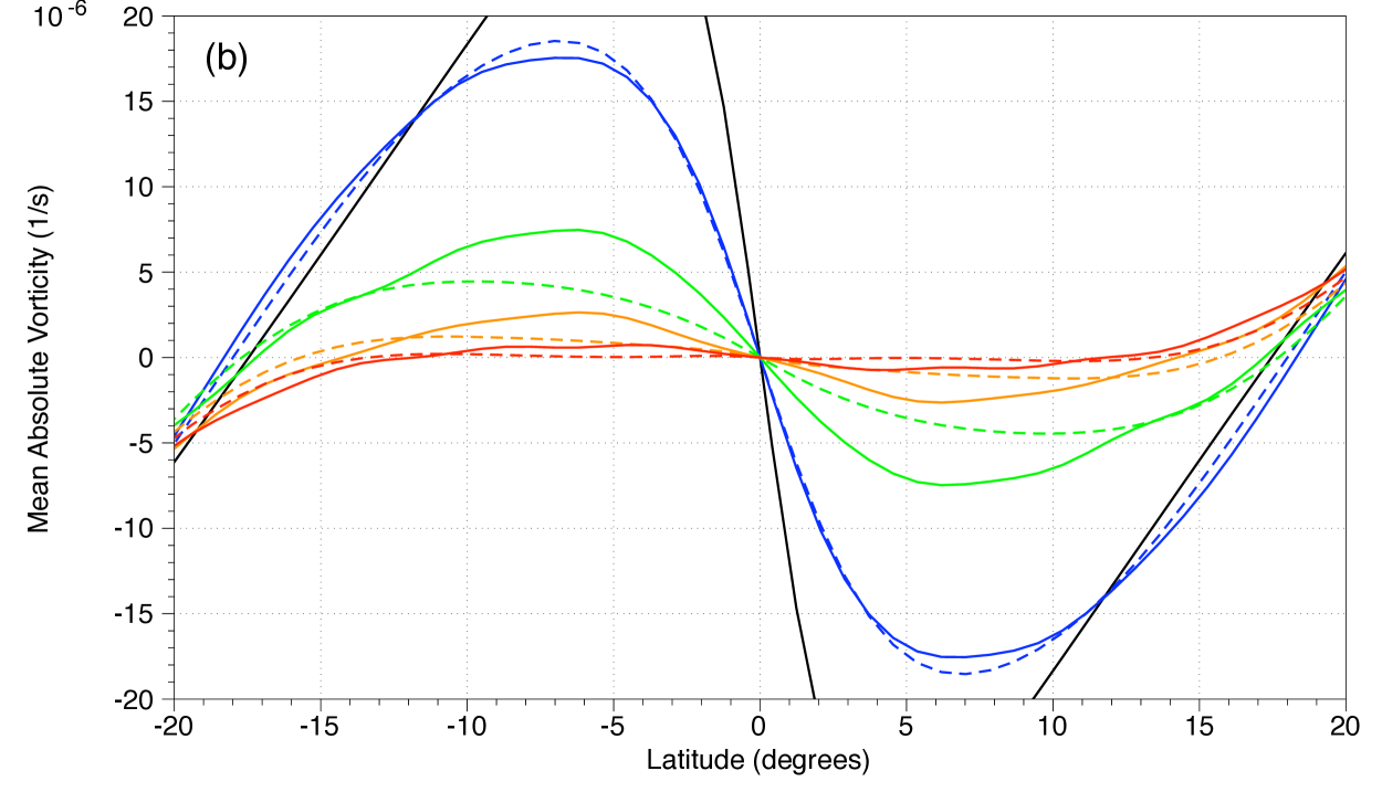
Figure 5: (a) Mean absolute vorticity $q_{1}$ as a function of latitude for different relaxation times. Zonally averaged results from DNS (solid lines) are compared to those from the CE (dashed lines). The black line ($\tau=0$) is the absolute vorticity of the fixed jet $q_{\rm jet}(\phi)$. (b) Magnified view of central jet region. Note the antisymmetry of the mean absolute vorticity (the first cumulant) under equatorial reflections.

The meridional profile (5) in our simulations is shown in Fig. 5 below. In the limiting zero-width case $\Delta\phi\rightarrow 0$ of a point jet,

$$\zeta_{\rm jet}(\phi)\equiv q_{\rm jet}(\phi)-f(\phi)=-\Gamma~{}{\rm sgn}(\phi)~{},$$ (6)

and the jet velocity has zonal and meridional components

$$u_{\rm jet}(\phi) = \Gamma a\tan(|\phi|/2-\pi/4),$$

$$v_{\rm jet}(\phi) = 0.$$ (7)

For $\Gamma>0$, the zonal velocity attains its most negative value $-\Gamma a$ at the equator.

For $\Gamma>0$, the gradient of the absolute vorticity (5) changes sign at the equator, so the jet satisfies the Rayleigh-Kuo necessary condition for inviscid barotropic instability. Lindzen et al. (1983) showed that the linear stability problem for the barotropic point jet on a $\beta$-plane is homomorphic to the Charney problem for baroclinic instability. The analog of the horizontal sign change of the absolute vorticity gradient in the barotropic problem is the vertical sign change of the generalized potential vorticity gradient in the baroclinic problem (with the generalized potential vorticity gradient including a singular surface contribution from the surface potential temperature gradient). What is the meridional coordinate in the barotropic problem corresponds to the vertical coordinate rescaled by the Prandtl ratio in the baroclinic problem.

The analogy to the baroclinic Charney problem motivated extensive study of the barotropic point-jet instability and its nonlinear equilibration, with the forcing and dissipation on the right-hand side of Eq. (3) as a barotropic analog of radiative forcing by Newtonian relaxation and Rayleigh drag (e.g., Schoeberl and Lindzen 1984; Nielsen and Schoeberl 1984; Schoeberl and Nielsen 1986; Shepherd 1988). Building on this body of work, here we focus on the statistically steady states of the flow and study their dependence on the relaxation time $\tau$. This allows us to test non-equilibrium closures systematically in two-dimensional barotropic flows that exhibit similar phenomena as analogous three-dimensional baroclinic flows, with the caveat, of course, that additional degrees of freedom in three-dimensional baroclinic flows, such as adjustment of the static stability, make the equilibration of baroclinic instabilities different from that of barotropic instabilities.

b Symmetries and conservation laws

Because the jet to which the flow relaxes is symmetric about the equator, steady-state statistics of the flow are hemispherically symmetric. Deviations from hemispheric symmetry can be used to gauge the degree of convergence towards statistically steady states. They will also highlight a qualitative problem with the statistics calculated by the CE (see section 5 below).

The EOM, Eq. (3), is invariant under a rotation of the azimuth, $\lambda\rightarrow\lambda+\alpha$, and under an inversion of the coordinates,

$$\phi \rightarrow -\phi$$

$$\lambda \rightarrow -\lambda$$

$$q \rightarrow q$$

$$q_{\rm jet} \rightarrow q_{\rm jet}\ .$$ (8)

Furthermore, the vorticities change sign under a north-south reflection about the equator,

$$\phi \rightarrow -\phi$$

$$\lambda \rightarrow \lambda$$

$$q \rightarrow -q$$

$$q_{\rm jet} \rightarrow -q_{\rm jet}~{}.$$ (9)

These symmetries are reflected in the statistics discussed below.

As a consequence of the constancy of the relaxation time $\tau$, statistically steady states satisfy two constraints that can be obtained by integrating the EOM over the domain. Kelvin’s circulation and Kelvin’s impulse of long-time averages $\langle\cdot\rangle$ in a statistically steady state are both equal to those of the jet to which the flow relaxes,

$$\int\langle q(\boldsymbol{\mathrm{r}},t)\rangle~{}d\boldsymbol{\mathrm{r}} = \int q_{\mathrm{jet}}~{}d\boldsymbol{\mathrm{r}},$$ (10)

$$\int\langle q(\boldsymbol{\mathrm{r}},t)\rangle\sin\phi~{}d\boldsymbol{\mathrm{r}} = \int q_{\mathrm{jet}}\sin\phi~{}d\boldsymbol{\mathrm{r}},$$ (11)

where $\boldsymbol{\mathrm{r}}\equiv(\phi,\lambda)$ is a position vector. Conservation of circulation (10) is trivially satisfied because vorticity integrals vanish at each moment in time,

$$\int q(\boldsymbol{\mathrm{r}},t)~{}d\boldsymbol{\mathrm{r}}=\int\zeta(\boldsymbol{\mathrm{r}},t)~{}d\boldsymbol{\mathrm{r}}=\int q_{\mathrm{jet}}(\boldsymbol{\mathrm{r}},t)~{}d\boldsymbol{\mathrm{r}}=0.$$ (12)

However, conservation of impulse (11), which is equivalent to conservation of the angular momentum about the rotation axis, is not trivial and must be respected by statistical closures.

3 Direct numerical simulation

a Parameters and implementation

All vorticities and their statistics can be expressed in units of $\Omega$, but to give a sense of scale, we set the rotation period to $2\pi/\Omega=1$ day. We use Arakawa’s (1966) energy- and enstrophy-conserving discretization scheme for the Jacobian on a $M\times N$ grid. For all results reported below, there are $M=400$ zonal points and $N=200$ meridional points. The lattice points are evenly spaced in latitude and longitude, apart from two polar caps that eliminate the coordinate singularities at the poles. Each cap subtends 0.15 radians ($8.6^{\circ}$) in angular radius and, following Arakawa, consists of a union of triangles radiating from the pole that match the grid along their base; scalar fields are constrained to be constant in each cap. At the initial time $t=0$, we set $q=q_{\rm jet}$ plus a small perturbation that breaks the azimuthal symmetry and triggers the instability. The time integration is then carried out with a standard second-order leapfrog algorithm using a time step of $\Delta t=15\,\mathrm{s}$. The accuracy of the numerical calculation was checked, in the absence of the jet, against exact analytic solutions that are available for special initial conditions (Gates and Riegel 1962). The jet parameters are fixed to be $\Gamma=0.6\Omega$ and $\Delta\phi=0.05$ radians ($2.9^{\circ}$). Though unphysically fast for Earth, the jet illustrates the strengths and shortcomings of the CE. Code implementing the numerical calculation is written in the Objective-C programming language, as its object orientation and dynamic typing are well suited for carrying out a comparison between DNS and the CE.

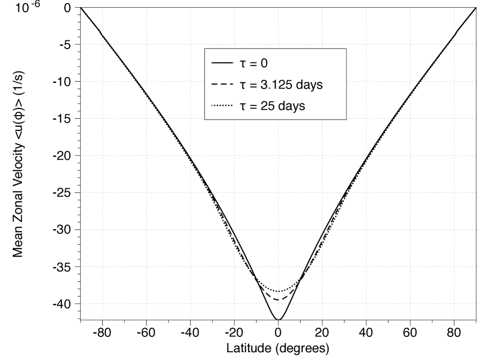
Figure 1: Mean zonal component of the velocity $\langle u(\phi)\rangle$ on a unit sphere of radius $a=1$. Relaxation times of $\tau=0$ [corresponding to the profile of the fixed jet $u_{\mathrm{jet}}(\phi)$], $3.125$ days, and $25$ days are plotted.

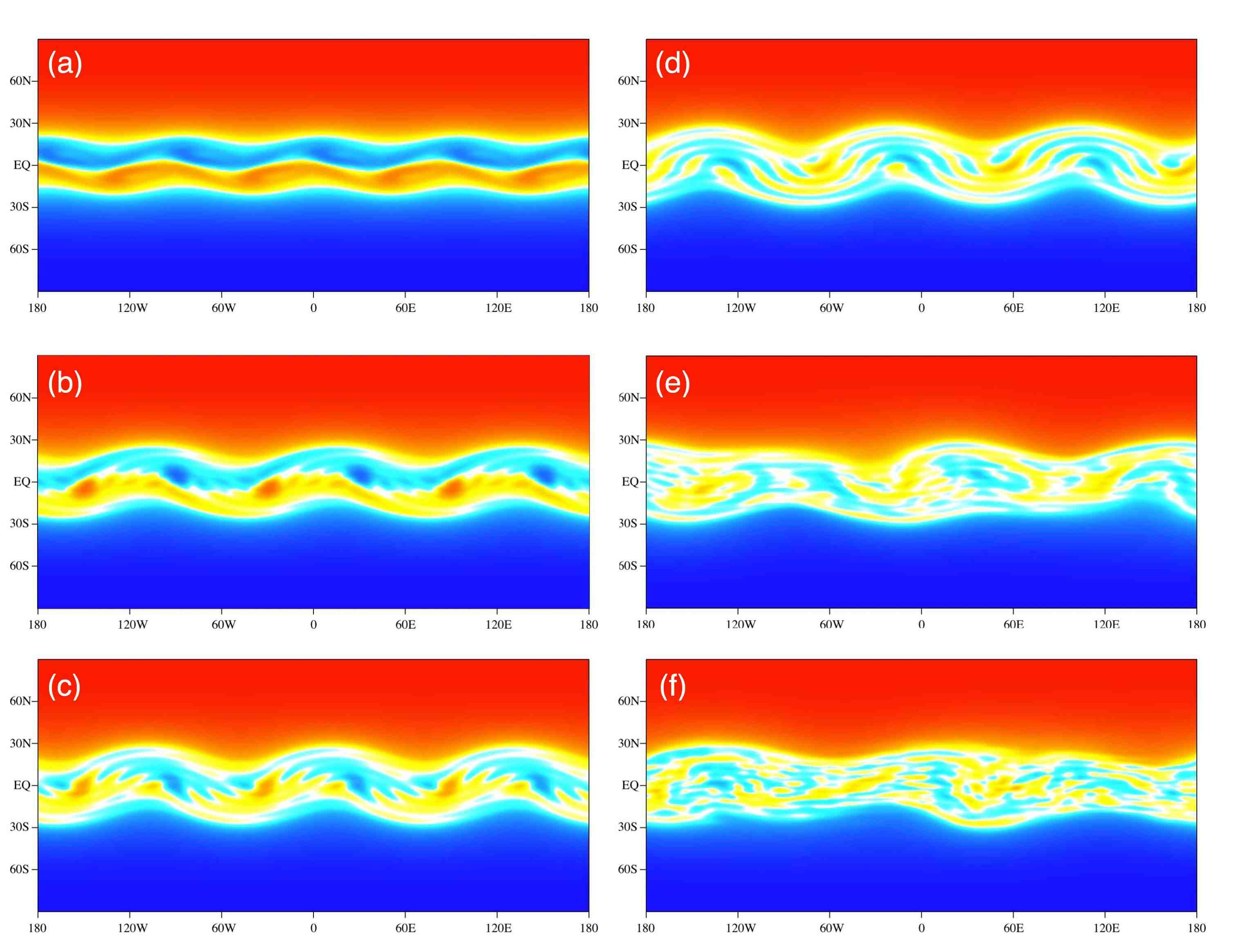
Figure 3: Snapshots of absolute vorticity in statistically steady states in a cylindrical projection. The relaxation times are (a) $\tau=1.5625$, (b) $3.125$, (c) $6.25$, (d) $12.5$, (e) $25$, and (f) $50$ days. As in Fig. 1, deep red (blue) corresponds to $q=\pm 10^{-4}$ s^-1.

Figure  1 shows the zonal velocity of the fixed jet $u_{\mathrm{jet}}(\phi)$ and the mean zonal velocity of the flow $\langle u(\phi)\rangle$ for two different relaxation times. Rounding of the jet due to mixing is evident. The absolute vorticity during the evolution of the instability and in the statistically steady state eventually reached in a typical DNS are shown in Fig. 2. Figure 3 displays snapshots of the absolute vorticity in the steady-state regime for six different choices of $\tau$. In the limit of vanishingly short relaxation time $\tau\rightarrow 0$ and strong coupling to the underlying jet, the fixed jet dominates, and $q=q_{\rm jet}$ with no fluctuations in the flow. For $\tau>0$, instabilities develop, and irreversible mixing begins to occur in critical-layer waves, which form Kelvin cats’ eyes that are advected zonally with the local mean zonal flow (e.g., Stewartson 1981; Maslowe 1986). At sufficiently large relaxation times ($\tau\gtrsim 12$ days), the jet becomes turbulent, and as $\tau$ increases further, turbulence increasingly homogenizes the absolute vorticity in a mixing region in the center of the jet. The dynamics are strongly out of equilibrium and nonlinear for intermediate values of $\tau$, yet continue to be statistically steady at long times. In the limit of long relaxation time $\tau\rightarrow\infty$ and weak coupling to the underlying jet, and upon addition of some small viscosity to the EOM, the system reaches an equilibrium configuration at long times (Salmon 1998; Turkington et al. 2001; Weichman 2006; Majda and Wang 2006), and again the fluctuations vanish. Here we restrict attention to the geophysically most relevant case of short and intermediate relaxation times.

Part of what makes this flow an interesting prototype problem to test statistical closures is that, except in the extreme limits of vanishing or infinite relaxation time, irreversible mixing is confined to the center of the jet and does not cover the domain. An estimate of the extent of the mixing region can be obtained by considering the state that would result by mixing absolute vorticity in the center of the jet such that it is, in the mean, homogenized there and continuous with the unmodified absolute vorticity of the underlying jet at the boundaries of the mixing region. Because of the symmetry of the jet, this state would have mean absolute vorticity

$$\langle q\rangle=\begin{cases}0&\text{for }|\phi|\leq\phi_{c},\\ q_{\mathrm{jet}}&\text{for }|\phi|\geq\phi_{c},\end{cases}$$ (13)

and the boundaries of the mixing region would be at the latitudes at which $q_{\mathrm{jet}}=0$, which are, with our parameter values, $\phi_{c}\approx\Gamma/(2\Omega)\approx 17^{\circ}$ (cf. Schoeberl and Lindzen 1984; Shepherd 1988). The meridional gradient of the resulting mean absolute vorticity does not change sign, so the corresponding flow would be stable according to the Rayleigh-Kuo criterion. It represents a zonal jet that is parabolic near the equator. However, while the mean absolute vorticity satisfies the circulation constraint (10) not only in the domain integral but integrated over the mixing region between $\pm\phi_{c}$, it does not satisfy the impulse constraint (11). To satisfy the impulse constraint, the mixing region in a statistically steady state extends beyond the latitudes $\phi_{c}$, as can be seen in Fig. 3 and will be discussed further below. Statistical closures must account for the structure of the transition between the mixing and no-mixing regions in this flow.

b Low-order equal-time statistics

The first cumulant (or first moment) $c_{1}$ of the relative vorticity depends only on latitude $\phi$, reflecting the azimuthal symmetry of the EOM,

$$c_{1}(\boldsymbol{\mathrm{r}})=\langle\zeta(\boldsymbol{\mathrm{r}})\rangle=c_{1}(\phi)~{}.$$ (14)

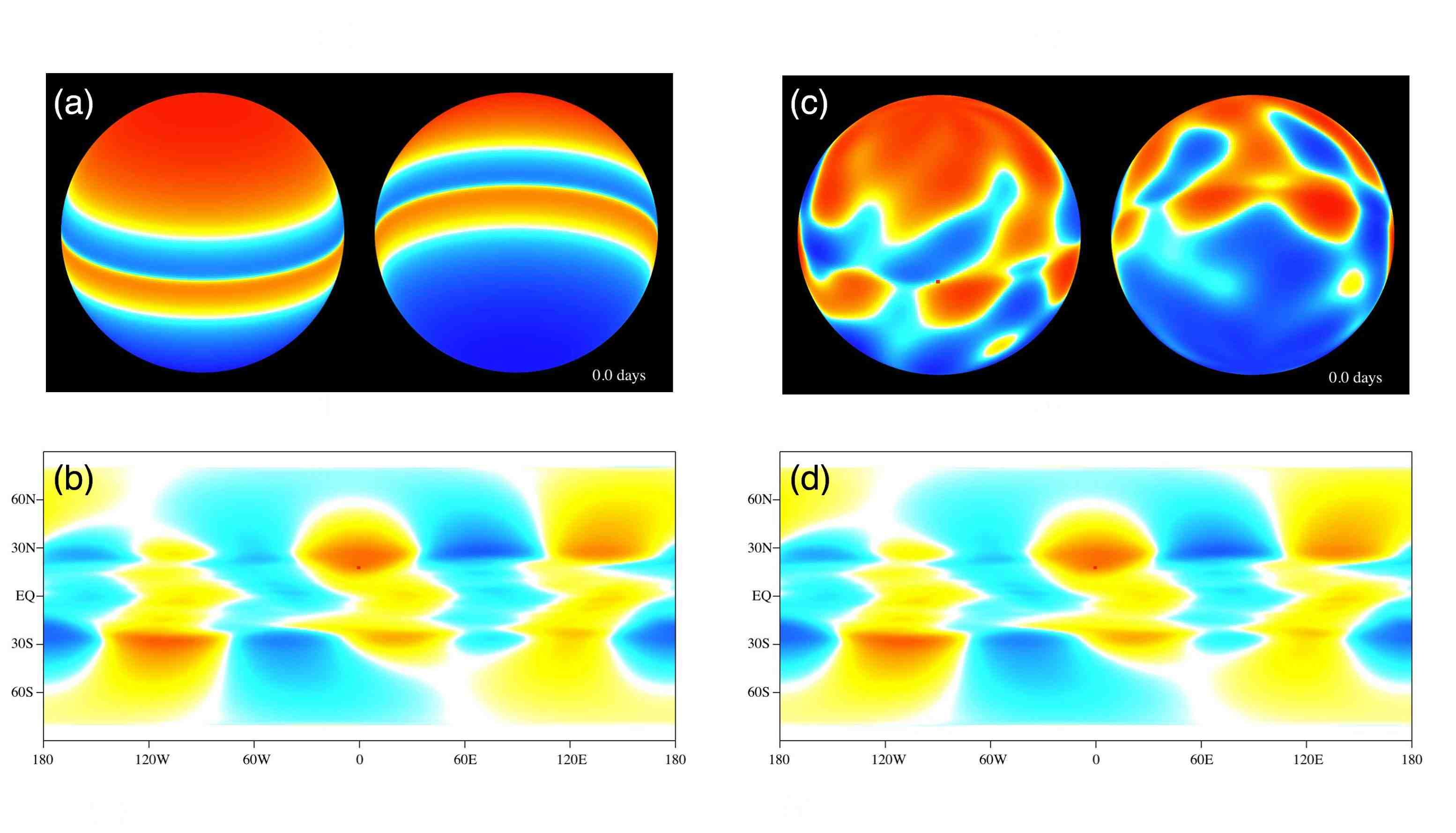
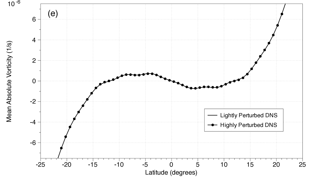
Figure 4: Different initial conditions yield the same low-order equal time statistics. The case of relaxation time $\tau=25$ days is illustrated. (a) Lightly perturbed initial absolute vorticity (from Fig. 1). (b) Second cumulant obtained from the lightly perturbed initial condition with reference point (orange square) positioned along the central meridian ($\lambda^{\prime}=0$) and at latitude $\phi^{\prime}=18^{\circ}$. Colors indicate positive (deep red is $10^{-10}$ s^-2) and negative (deep blue is $-10^{-10}$ s^-2) correlations with respect to the reference point. (c) Highly perturbed initial condition. (d) Second cumulant obtained from the highly perturbed initial condition. (e) Comparison of the zonally averaged mean absolute vorticity in the central jet region.

It is also convenient to define the first moment of the absolute vorticity, $q_{1}(\phi)\equiv\langle q(\boldsymbol{\mathrm{r}})\rangle=c_{1}(\phi)+f(\phi)$. The calculation of the time averages $\langle\cdot\rangle$ commences once the jet has reached a statistically steady state. As the adjustment of the mean flow is controlled by the relaxation time $\tau$, reaching a statistically steady state takes longer for larger $\tau$. Statistics are then accumulated every $100$ minutes for a minimum of $100$ days of model time, until adequate convergence is obtained. We have verified that the long-time averages thus obtained are typically independent of the particular choice of initial condition; see, for instance, Fig. 4. (The one exception is the case of $\tau=3.125$ days, in which, depending on initial conditions, critical-layer waves of wavenumber three or four are present in the statistically steady states. As the wavenumber-three mode has slightly lower kinetic energy, and is reached from strongly perturbed initial conditions, we focus on it here.) As expected, azimuthal symmetry is recovered in such long time-averages, as can be seen, for instance, in the final panel of Fig. 2. In addition, the first cumulant changes sign under reflections about the equator,

$$c_{1}(-\phi)=-c_{1}(\phi)\ ,$$ (15)

a consequence of the reflection symmetry (9).

The second cumulant of the relative vorticity, given in terms of its first and second moments by

$$c_{2}(\boldsymbol{\mathrm{r}},\boldsymbol{\mathrm{r}}^{\prime})=\langle\zeta(\boldsymbol{\mathrm{r}})~{}\zeta(\boldsymbol{\mathrm{r}}^{\prime})\rangle_{C}\equiv\langle\zeta(\boldsymbol{\mathrm{r}})~{}\zeta(\boldsymbol{\mathrm{r}}^{\prime})\rangle-\langle\zeta(\boldsymbol{\mathrm{r}})\rangle\langle\zeta(\boldsymbol{\mathrm{r}}^{\prime})\rangle\ ,$$ (16)

depends on the latitude of both points $\boldsymbol{\mathrm{r}}$ and $\boldsymbol{\mathrm{r}}^{\prime}$, but only on the difference in the longitudes:

$$c_{2}(\boldsymbol{\mathrm{r}},\boldsymbol{\mathrm{r}}^{\prime})=c_{2}(\phi,\phi^{\prime},\lambda-\lambda^{\prime})\ .$$ (17)

It is essential to take advantage of the azimuthal symmetry of the second cumulant, Eq. (17), to reduce the amount of memory required to store the second cumulants by a factor of $M$, from $M^{2}N^{2}$ to $MN^{2}$ scalars. In the DNS, the reduction is realized by averaging the second cumulant over $\lambda^{\prime}$ for each value of $\Delta\lambda\equiv\lambda-\lambda^{\prime}$. The averaging also improves the accuracy of the statistic.

By definition, the second cumulant is symmetric under an interchange of coordinates, $c_{2}(\boldsymbol{\mathrm{r}},\boldsymbol{\mathrm{r}}^{\prime})=c_{2}(\boldsymbol{\mathrm{r}}^{\prime},\boldsymbol{\mathrm{r}})$. It also possesses the discrete symmetry

$$c_{2}(-\phi,-\phi^{\prime},\Delta\lambda)=c_{2}(\phi,\phi^{\prime},\Delta\lambda)~{},$$ (18)

a consequence of the reflection operation (9).

4 Second-order cumulant expansion

The jets considered here are inhomogeneous and possess nontrivial mean flows. As a consequence, the leading-order nonlinearity is the interaction between the mean flow and eddies (fluctuations about the mean flow), and already the mean flow, a first-order statistic, is of interest in closure theories (e.g. Schoeberl and Lindzen 1984). In contrast, the leading-order nonlinearity in homogeneous flows is the interaction of eddies with each other, and only higher-order statistics are of interest in closure theories. Many higher-order closure approximations impose a requirement of homogeneity (e.g., Holloway and Hendershott 1977; Legras 1980; Huang et al. 2001) and are not directly applicable to systems with inhomogeneous flows.

The second-order closure we consider is based on an expansion of vorticity statistics in equal-time cumulants. The cumulant expansion can be formulated either using the Hopf functional approach (Frisch 1995; Ma and Marston 2005) or by a standard Reynolds decomposition of each scalar field into a mean component plus fluctuations or eddies (denoted with a prime):

$$q(\boldsymbol{\mathrm{r}}) = \langle\zeta(\boldsymbol{\mathrm{r}})\rangle+f(\phi)+\zeta^{\prime}(\boldsymbol{\mathrm{r}})$$

$$\psi(\boldsymbol{\mathrm{r}}) = \langle\psi(\boldsymbol{\mathrm{r}})\rangle+\psi^{\prime}(\boldsymbol{\mathrm{r}})\ .$$ (19)

The EOMs for the first and second cumulants may be written most conveniently by introducing the following auxiliary statistical quantities:

$$p_{1}(\boldsymbol{\mathrm{r}}) \equiv \langle\psi(\boldsymbol{\mathrm{r}})\rangle$$

$$p_{2}(\boldsymbol{\mathrm{r}},\boldsymbol{\mathrm{r}}^{\prime}) \equiv \langle\psi(\boldsymbol{\mathrm{r}})\zeta(\boldsymbol{\mathrm{r}}^{\prime})\rangle_{C}$$ (20)

$$= \langle\psi^{\prime}(\boldsymbol{\mathrm{r}})\zeta^{\prime}(\boldsymbol{\mathrm{r}}^{\prime})\rangle\ .$$

These quantities contain no new information as $c_{1}=\nabla^{2}p_{1}$ and $c_{2}=\nabla^{2}p_{2}$, where it is understood that unprimed differential operators such as $\nabla^{2}$ and $J[~{},~{}]$ act only on the unprimed coordinates $\boldsymbol{\mathrm{r}}$. Substituting Eq. (19) into Eq. (3) and applying the averaging operation $\langle\cdot\rangle$ yields the EOM for the first moment or cumulant:

$${{\partial c_{1}(\boldsymbol{\mathrm{r}})}\over{\partial t}} = J[c_{1}(\boldsymbol{\mathrm{r}})+f(\phi),~{}p_{1}(\boldsymbol{\mathrm{r}})]+\int J[\delta^{2}(\boldsymbol{\mathrm{r}}-\boldsymbol{\mathrm{r}}^{\prime}),~{}p_{2}(\boldsymbol{\mathrm{r}},\boldsymbol{\mathrm{r}}^{\prime})]~{}d\boldsymbol{\mathrm{r}}^{\prime}+\frac{\zeta_{\rm jet}(\phi)-c_{1}(\boldsymbol{\mathrm{r}})}{\tau}\ .$$

(21)

Here partial integration over $\boldsymbol{\mathrm{r}}^{\prime}$ has been used to group $\psi^{\prime}$ and $\zeta^{\prime}$ that appear as separate arguments of the Jacobian operator into the statistical quantity $p_{2}$. Similarly, multiplication of Eq. (3) by $\zeta^{\prime}(\boldsymbol{\mathrm{r}}^{\prime})$ followed by averaging yields the EOM for the second cumulant, which upon discarding the term cubic in the fluctuations may be written as

$${{\partial c_{2}(\boldsymbol{\mathrm{r}},\boldsymbol{\mathrm{r}}^{\prime})}\over{\partial t}} = J[c_{1}(\boldsymbol{\mathrm{r}})+f(\phi),~{}p_{2}(\boldsymbol{\mathrm{r}},\boldsymbol{\mathrm{r}}^{\prime})]+J[c_{2}(\boldsymbol{\mathrm{r}},\boldsymbol{\mathrm{r}}^{\prime}),~{}p_{1}(\boldsymbol{\mathrm{r}})]-\frac{c_{2}(\boldsymbol{\mathrm{r}},\boldsymbol{\mathrm{r}}^{\prime})}{\tau}+(\boldsymbol{\mathrm{r}}\leftrightarrow\boldsymbol{\mathrm{r}}^{\prime}),$$

where $(\boldsymbol{\mathrm{r}}\leftrightarrow\boldsymbol{\mathrm{r}}^{\prime})$ is shorthand notation for terms that maintain the symmetry $c_{2}(\boldsymbol{\mathrm{r}},\boldsymbol{\mathrm{r}}^{\prime})=c_{2}(\boldsymbol{\mathrm{r}}^{\prime},\boldsymbol{\mathrm{r}})$. Closure has been achieved at second order in the expansion by constraining the third and higher cumulants to be zero

$$c_{3}=\langle\zeta(\boldsymbol{\mathrm{r}})~{}\zeta(\boldsymbol{\mathrm{r}}^{\prime})~{}\zeta(\boldsymbol{\mathrm{r}}^{\prime\prime})\rangle_{C}=0,\ {\rm etc.}$$ (23)

Otherwise an additional term would appear in Eq. (LABEL:2ndCumulantEOM) that couples the second and third cumulants. The closure approximation $c_{3}=0$ amounts to neglecting eddy-eddy interactions while retaining eddy-mean flow interactions (e.g., Herring 1963; Schoeberl and Lindzen 1984).

The EOMs for the two cumulants are integrated numerically using the same algorithms and methods as those employed for DNS, starting from the initial conditions $c_{1}(\boldsymbol{\mathrm{r}})=\zeta_{\rm jet}(\boldsymbol{\mathrm{r}})$ and $c_{2}(\boldsymbol{\mathrm{r}},\boldsymbol{\mathrm{r}}^{\prime})=c~{}\delta^{2}(\boldsymbol{\mathrm{r}}-\boldsymbol{\mathrm{r}}^{\prime})-c/4\pi$ with small positive $c$. The cumulants evolve toward the fixed point

$${{\partial c_{1}(\boldsymbol{\mathrm{r}})}\over{\partial t}}={{\partial c_{2}(\boldsymbol{\mathrm{r}},\boldsymbol{\mathrm{r}}^{\prime})}\over{\partial t}}=0\ .$$ (24)

As a practical matter, we consider that the fixed point has been reached when the cumulants do not change significantly with further time evolution. It is essential for the second cumulant to have an initial non-zero value as otherwise it would be zero for all time, corresponding to axisymmetric flow, which is unstable with respect to non-axisymmetric perturbations.

The programming task of solving the equations of motion for the cumulants is simplified by implementing the CE as a subclass of the DNS class, inheriting all of the lattice DNS methods without modification. The azimuthal symmetry of the statistics, Eqs. (14) and (17), and the discrete symmetries, Eqs. (15) and (18), are exploited to reduce the amount of memory required to store $c_{2}$ and $p_{2}$. The symmetries also speed up the calculation and help thwart the development of numerical instabilities. The time step $\Delta t$ is permitted to adapt, increasing as the fixed point is reached. Various consistency checks on the numerical solution are performed during the course of the time integration. For instance we verify that

$$c_{2}(\boldsymbol{\mathrm{r}},\boldsymbol{\mathrm{r}})=c_{2}(\phi,\phi,\Delta\lambda=0)\geq 0$$ (25)

at all lattice points $\boldsymbol{\mathrm{r}}$. Furthermore from Eq. (12) it must be the case that

$$\int c_{1}(\boldsymbol{\mathrm{r}})~{}d\boldsymbol{\mathrm{r}}=\int c_{2}(\boldsymbol{\mathrm{r}},\boldsymbol{\mathrm{r}}^{\prime})~{}d\boldsymbol{\mathrm{r}}=0\ .$$ (26)

Likewise, as the second-order cumulant expansion conserves Kelvin’s impulse, it follows from the impulse constraint (11) that

$$\int c_{1}(\boldsymbol{\mathrm{r}})\sin(\phi)~{}d\boldsymbol{\mathrm{r}}=\int q_{\rm jet}(\phi)\sin(\phi)~{}d\boldsymbol{\mathrm{r}}$$ (27)

and

$$\int c_{2}(\boldsymbol{\mathrm{r}},\boldsymbol{\mathrm{r}}^{\prime})\sin(\phi)~{}d\boldsymbol{\mathrm{r}}=0~{}.$$ (28)

Finally the local mean kinetic energy is non-negative,

$$\langle E(\boldsymbol{\mathrm{r}})\rangle=-p_{2}(\boldsymbol{\mathrm{r}},\boldsymbol{\mathrm{r}})-p_{1}(\boldsymbol{\mathrm{r}})c_{1}(\boldsymbol{\mathrm{r}})\geq 0,$$ (29)

because the statistics governed by Eqs. (21) and (LABEL:2ndCumulantEOM) are realizable: They can be obtained from a linear equation of motion for the vorticity that is driven by Gaussian stochastic forcing (Orszag 1977; Salmon 1998). The total kinetic energy obtained by CE compares well to that determined by DNS.

5 Comparison between DNS and CE

The equal-time statistics accumulated in the DNS can be directly compared to the results of the CE because both calculations are based on the same jet model with the same finite-difference approximations on the same $M\times N$ lattice. Thus any differences between the DNS and CE statistics may be ascribed solely to the closure approximation. Results similar to those below are obtained on a coarser $200\times 100$ lattice.

Figure 5 shows the mean absolute vorticity calculated with the two approaches. Closest agreement between DNS and the CE is found at the shortest relaxation time of $\tau=1.5626$ days. The CE is accurate for short relaxation times because fluctuations are suppressed by the strong coupling to the fixed jet. The second cumulant is reduced in size, and errors introduced by the closure approximation that neglects the third cumulant are small. For longer relaxation times, the CE systematically flattens out the mean absolute vorticity in the center of the jet too strongly. The largest absolute discrepancy in the mean vorticity appears at an intermediate relaxation time of $\tau=3.125$ days. At longer relaxation times, the mean absolute vorticities in the DNS and CE become small in the central jet region; however, their fractional discrepancy increases, and the second cumulants show increasing quantitative and even qualitative discrepancies.

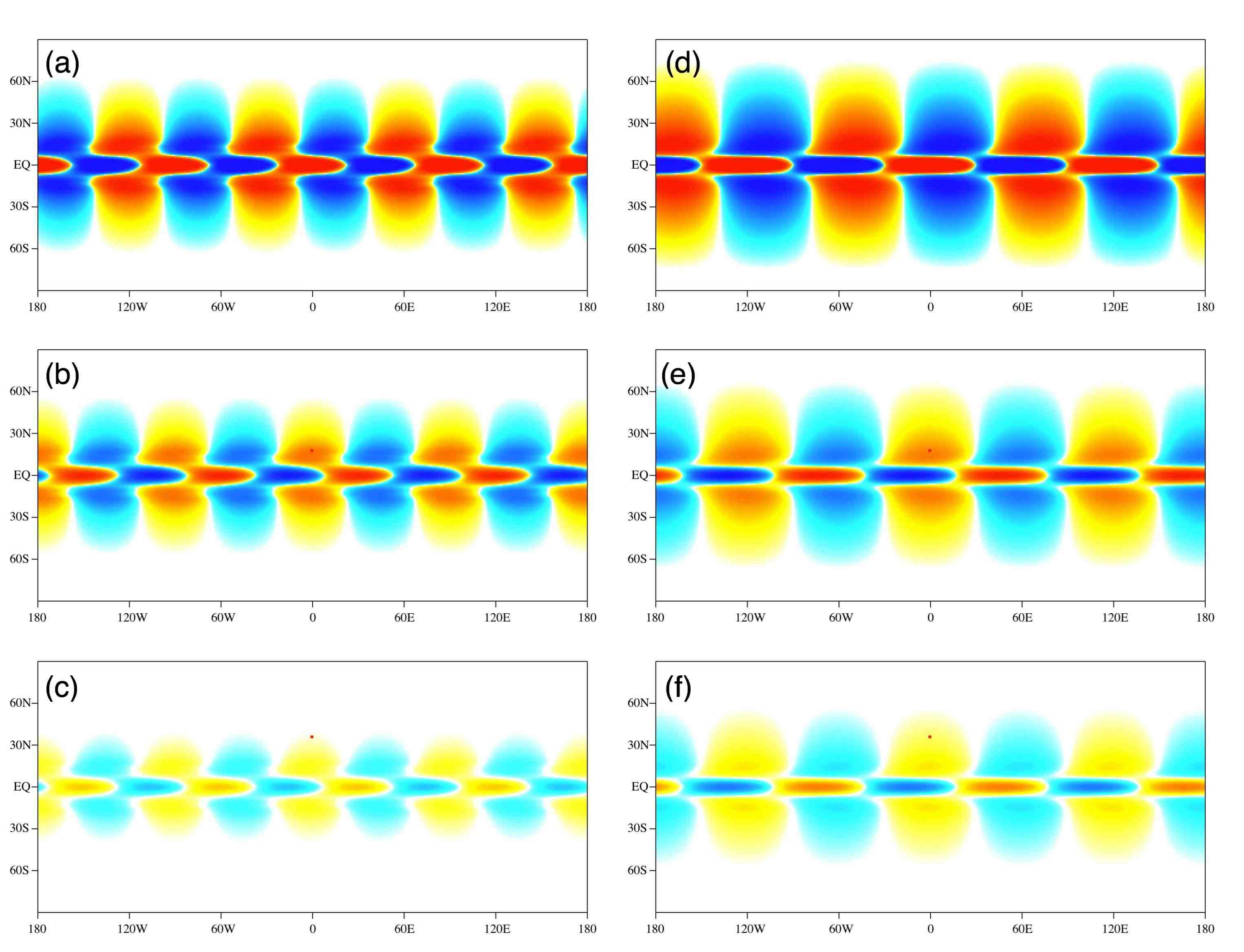
Figure 6: The second cumulant of the relative vorticity field, $c_{2}(\phi,\phi^{\prime},\lambda-\lambda^{\prime})$, for relaxation time $\tau=1.5625$ days. (a), (b) and (c): DNS. (d), (e), and (f): CE. The reference point (orange square) is positioned along the central meridian ($\lambda^{\prime}=0$) and at latitudes of $\phi^{\prime}=0$ for (a) and (d), $\phi^{\prime}=18^{\circ}$ for (b) and (e), and $\phi^{\prime}=36^{\circ}$ for (c) and (f). Colors indicate positive (deep red is $10^{-10}$ s^-2) and negative (deep blue is $-10^{-10}$ s^-2) correlations with respect to the reference point.

Comparison of the second cumulants for $\tau=1.5625$ days (Fig. 6) reveals a qualitative discrepancy. The two-point correlations as calculated in the CE exhibit wavenumber-three periodicity, in disagreement with the wavenumber-four periodicity of the critical-layer wave dominating the fluctuating flow component in DNS (Fig 3). In this regard, the CE mimics the wavenumber-three periodicity found in DNS at the longer relaxation times. In both DNS and CE, the correlations are strongest in absolute value when one of the two points of the second cumulant is located near the equator. Interestingly, the second cumulant from the DNS exhibits a near-exact symmetry that is not a symmetry of the EOM,

$$c_{2}(-\phi,\phi^{\prime},\Delta\lambda)\approx c_{2}(\phi,\phi^{\prime},\Delta\lambda)~{},$$ (30)

in addition to the symmetries of Eqs. (15) and (18). This approximate symmetry, which holds exactly for the second-order CE, may be attributed in the case of the DNS to the small size of the third cumulant. The fixed point of the second-order CE as described by Eqs. (21), (LABEL:2ndCumulantEOM), and (24) possesses the artificial symmetry, for under the north-south reflection $\phi\rightarrow-\phi$ the Jacobian operator (4) changes sign, as do both $c_{1}(\phi)$ and $p_{1}(\phi)$, and the fixed point equations remain unchanged provided that the second cumulant obeys Eq. (30). The artificial symmetry would, however, be broken in general by any coupling of the second cumulant to a third (non-zero) cumulant or, equivalently, by the inclusion of eddy-eddy interactions, which can redistribute eddy enstrophy spatially. Thus the artificial symmetry (30) is an artifact of the closure (23).

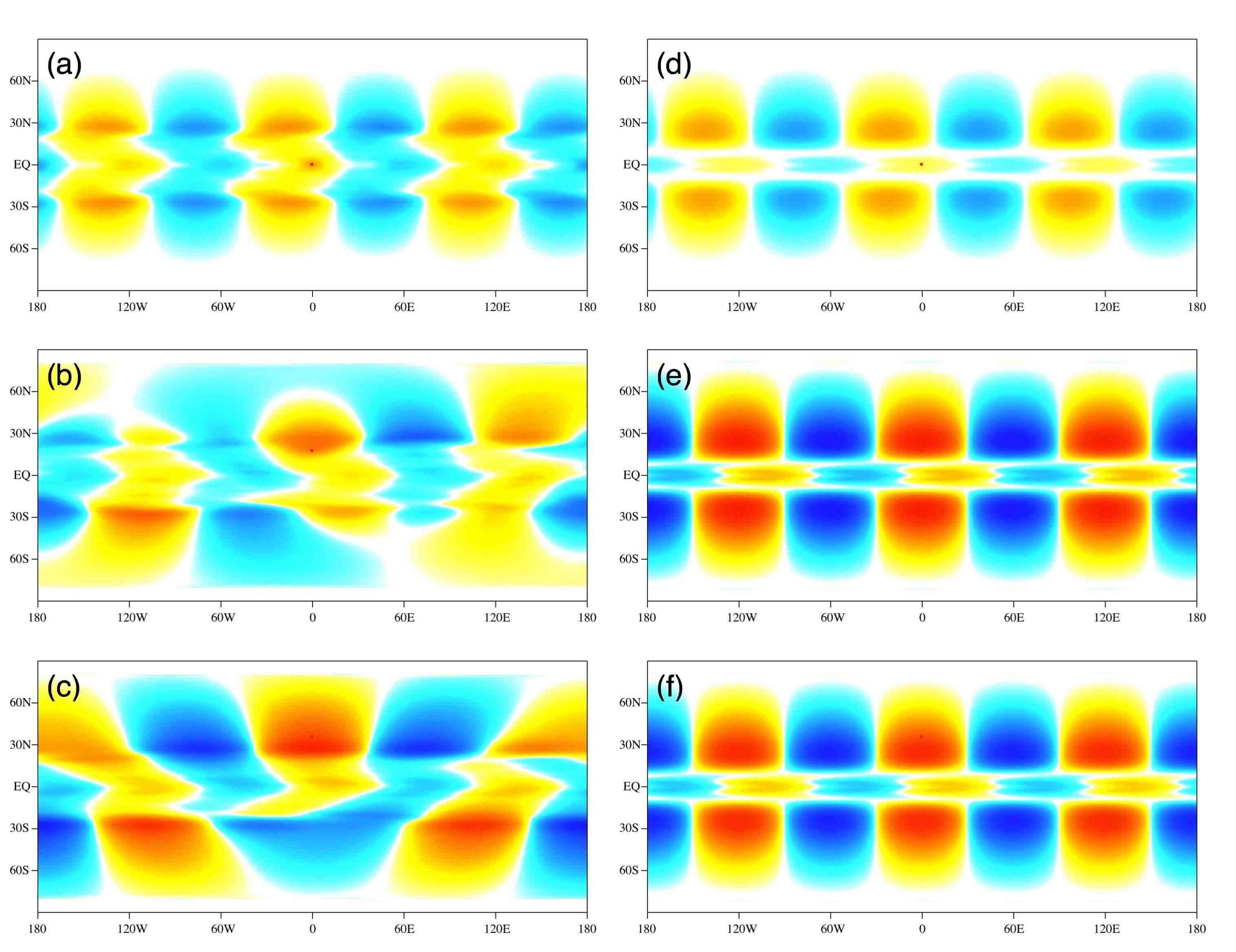
Figure 7: Same as Fig. 5 except for a relaxation time of $\tau=25$ days. The reflection symmetry about the equator seen in the CE, an artifact of the closure truncation, is not present in the DNS.

Other qualitative discrepancies appear at longer relaxation times (Fig. 7). For $\tau=25$ days, the second cumulant calculated by DNS no longer shows the artificial symmetry (30), whereas the symmetry continues to be present in the CE due to the closure approximation. In contrast to the $\tau=1.5625$ case, the largest two-point correlations occur when one of the two points is away from the equator, reflecting the fact that correlations are washed out by the strong turbulence near the jet center. Finally, the second cumulant as calculated by CE shows a wavenumber-three periodicity, with excessively strong correlations at large separations, as a result of the neglect of eddy-eddy interactions, which strongly distort the eddy fields in the DNS. Nonetheless, even for relatively long relaxation times for which differences between the CE and the DNS at the center of the jet are apparent, the CE does capture the structure of the transition from the mixing region in the center of the jet to the non-mixing region away from the center, where the mean absolute vorticity in the DNS and the absolute vorticity of the underlying jet coincide.

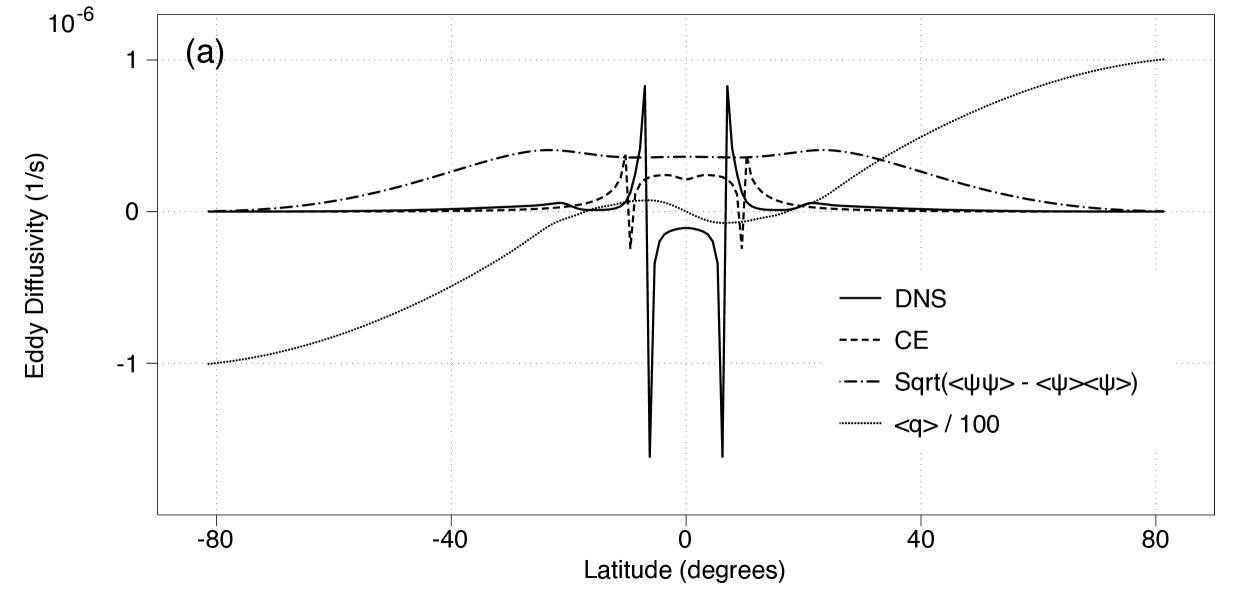
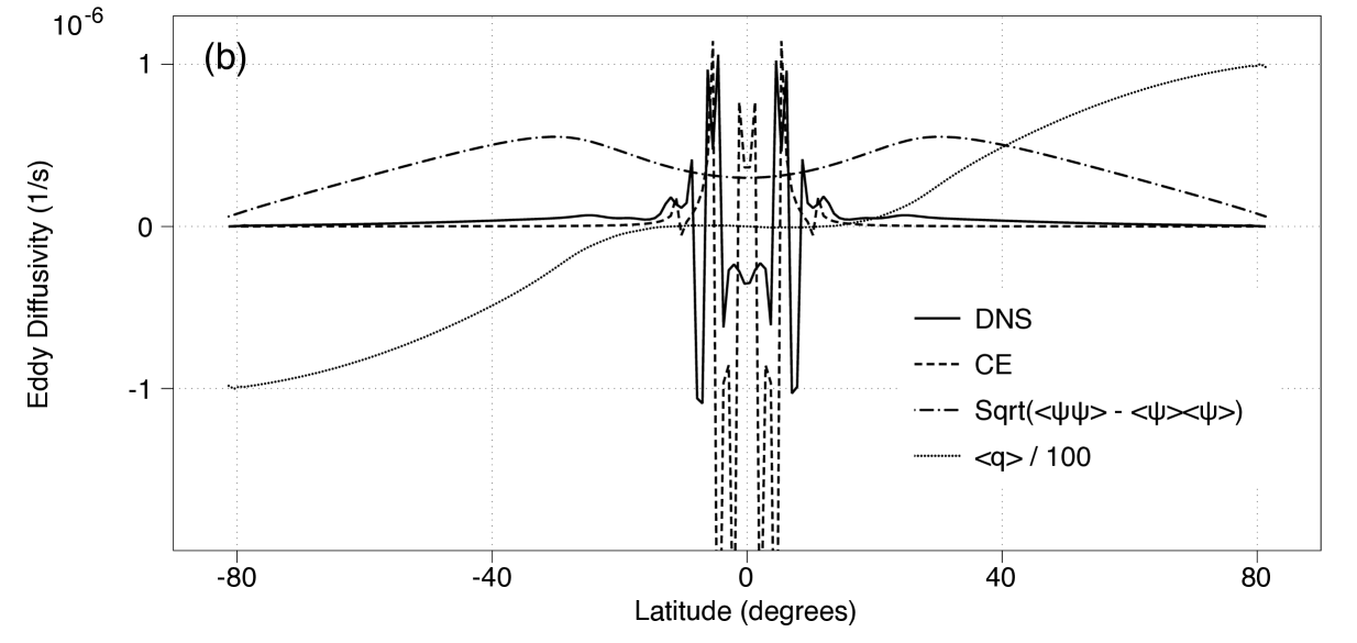
Figure 8: (a) Eddy diffusivity $\kappa$ for the case of relaxation time $\tau=3.125$ days on the unit sphere ($a=1$) as calculated by DNS and CE. Also plotted for comparison are the DNS calculation of the square root of the variance in the streamfunction, $\sqrt{\langle\psi^{2}(\boldsymbol{\mathrm{r}})\rangle-\langle\psi(\boldsymbol{\mathrm{r}})\rangle^{2}}$, and the first moment of the absolute vorticity. (b) Same as (a) except for $\tau=25$ days.

Figure 8 compares the eddy diffusivity $\kappa$ of absolute vorticity in the meridional direction as calculated by DNS and CE for the two cases of $\tau=3.125$ and $25$ days. The diffusivity is defined by second-order statistics:

$$\kappa(\phi) =-\langle v^{\prime}(\boldsymbol{\mathrm{r}})q^{\prime}(\boldsymbol{\mathrm{r}})\rangle\left(\frac{\partial\langle q(\boldsymbol{\mathrm{r}})\rangle}{\partial(a\phi)}\right)^{-1}$$ (DNS)

$$=\frac{1}{\cos\phi}\frac{\partial p_{2}(\phi,\phi,\Delta\lambda)}{\partial(\Delta\lambda)}\left(\frac{\partial q_{1}(\phi)}{\partial\phi}\right)^{-1} \text{(CE)}.$$ (31)

The diffusivities calculated by the two methods are qualitatively similar: diffusion is largely confined to the mixing region of the jet; it is negative near critical layers within the mixing region (cf. Schoeberl and Lindzen 1984). However, there are significant quantitative differences between DNS and CE, as might be expected given that second-order statistics will generally be poorly reproduced in a second-order closure.

6 Discussion and conclusions

The barotropic flows considered here attain statistically steady states after sufficient time has passed. They are out of equilibrium on large scales as the fixed zonal jet to which they relax is both a source and a sink of energy. Statistical approaches that have been developed to describe the equilibrium states of geophysical flows in the absence of large-scale forcing and dissipation therefore are not applicable here. For example, approaches based on maximizing an entropy functional subject to constraints on energy, enstrophy, and possibly higher-order inviscid invariants (Miller 1990; Robert and Sommeria 1991; Salmon 1998; Turkington et al. 2001; Weichman 2006; Majda and Wang 2006) assume ergodic mixing and therefore would give statistical equilibrium states with mixing throughout the domain, rather than mixing confined to the region in the center of the jet.

One-point closures likewise are generally not adequate for the inhomogeneous flows we considered. For example, as one ingredient of a diffusive one-point closure one might postulate a linear relationship between an eddy diffusivity $\kappa(\phi)$ and rms fluctuations in the streamfunction $\sqrt{\langle\psi^{2}(\boldsymbol{\mathrm{r}})\rangle-\langle\psi(\boldsymbol{\mathrm{r}})\rangle^{2}}$, which has the same physical dimension (Holloway and Kristmannsson 1984; Holloway 1986; Stammer 1998). Figure 8 reveals that fluctuations in the streamfunction persist to much higher latitudes owing to Rossby wave dynamics outside the mixing region. A diffusive closure in which the diffusivity is a linear function of rms streamfunction fluctuations would therefore also lead to mean states with mixing in an overly large fraction of the domain.

We have tested the simplest non-trivial two-point closure approximation based on a cumulant expansion of vorticity statistics, obtained by discarding the third and higher cumulants. This corresponds to neglecting eddy-eddy interactions while retaining eddy-mean flow interactions. The second-order CE is realizable, has no adjustable parameters (such as eddy damping terms), and is not restricted to homogeneous flows. For short relaxation times, the expansion reproduces the first moment fairly accurately. For longer relaxation times, it is quantitatively less accurate, but it still captures the transition from a mixing region at the center of the jet to a no-mixing region away from the center.

The steady-state statistics from the CE can be found with much less computational effort than that required to calculate time-averaged statistics using DNS, as the partial differential equations governing the fixed point (24) are time-independent. This is especially true if a good initial guess is available for the cumulants $c_{1}$ and $c_{2}$ because the fixed point can then be reached rapidly by iteration. Furthermore, as the statistics vary much more slowly in space than any given realization of the underlying dynamics (see Fig. 2), it may be possible to employ coarser grids without sacrificing accuracy. Thus the CE realizes a program envisioned by Lorenz (1967) long ago by solving directly for the statistics, but it does so at the cost of a closure approximation that compromises the accuracy of the statistics, especially for flows with more strongly nonlinear eddy-eddy interactions. There is evidence, however, that nonlinear eddy-eddy interactions in Earth’s atmosphere are weak (Schneider and Walker 2006). O’Gorman and Schneider (2007) have shown that several features of atmospheric flows, such as scales of jets and the shape of the atmospheric turbulent kinetic energy spectrum, can be recovered in an idealized general circulation model in which eddy-eddy interactions are suppressed. In particular, baroclinic jets form spontaneously and are maintained by eddy-mean flow interactions even in the absence of nonlinear eddy-eddy interactions. So a second-order CE may be worth exploring for more realistic models. Extensions of the CE to multi-layer models governed by either quasigeostrophic dynamics or the primitive equations are straightforward. The storage requirement for the second cumulant grows as the square of the number of layers, but it remains feasible so long as the models retain azimuthal symmetry. The incorporation of topography and other symmetry-breaking effects is more problematic because of the much larger storage requirement.

Whether more sophisticated closures can be devised that are more accurate and yet only require comparable computational effort remains an open question. In the case of isotropic turbulence, renormalization-group inspired closures show some promise (McComb 2004), but these typically make extensive use of translation invariance in actual calculations. Investigation of more sophisticated approximations for non-isotropic and inhomogeneous systems, such as the barotropic flows we considered, may be warranted in view of the partial success of the cumulant expansion reported here.

Acknowledgments.

We thank Greg Holloway, Paul Kushner, Ookie Ma, and Peter Weichman for helpful discussions. This work was supported in part by the National Science Foundation under grants DMR-0213818 and DMR-0605619. It was initiated during the Summer 2005 Aspen Center for Physics workshop “Novel Approaches to Climate,” and J. B. M. and T. S. thank the Center for its support.

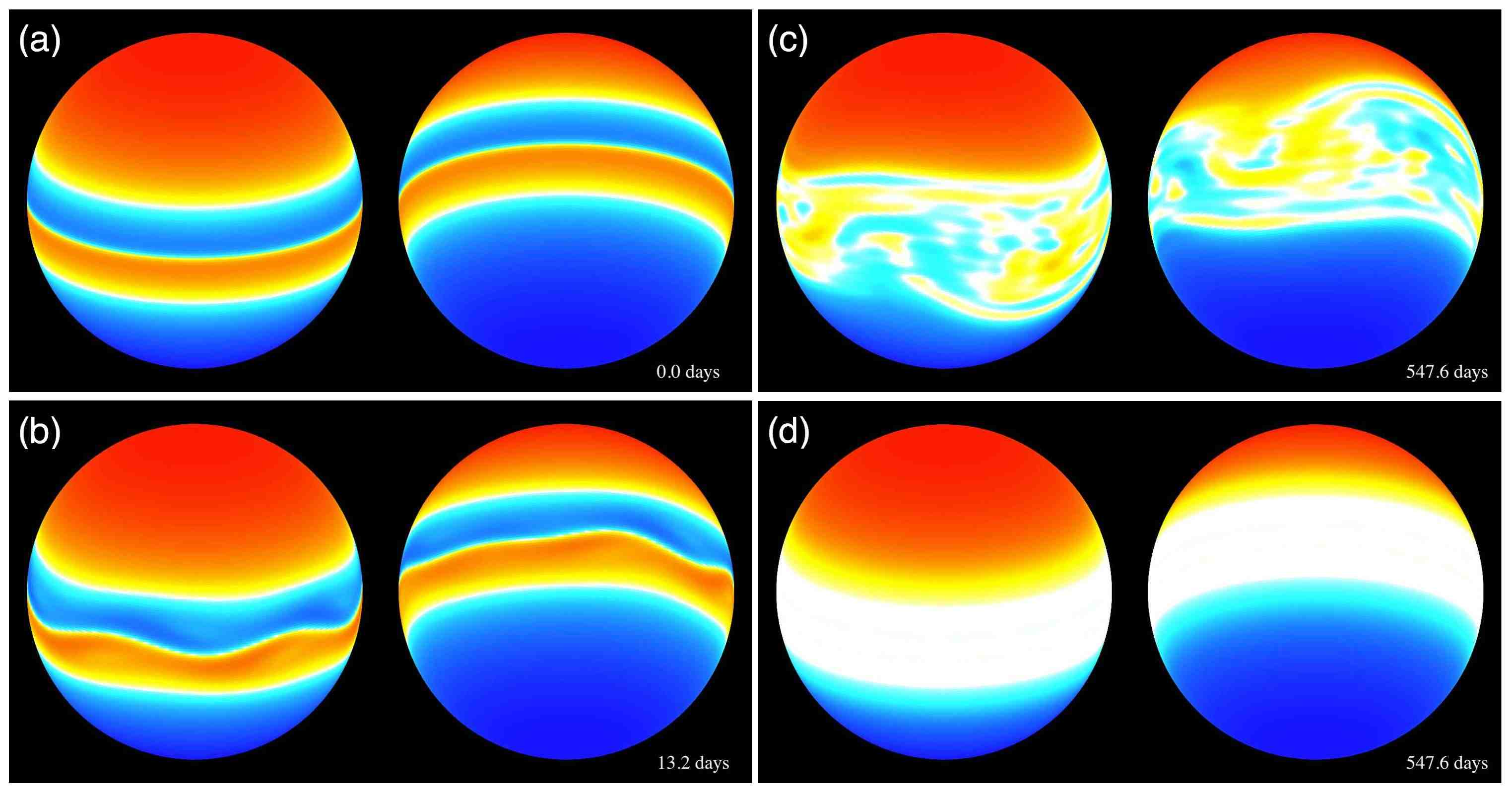
Figure 2: Absolute vorticity $q$ as calculated by DNS for a relaxation time of $\tau=25$ days. The left and right hemispheres are shown in each panel; each is inclined by $20^{\circ}$ to make the poles visible. Deep red (blue) corresponds to $q=\pm 10^{-4}$ s^-1. (a) Initial state with equatorial zonal jet. (b) Early development of instability. (c) Statistically steady state. (d) Mean absolute vorticity $q_{1}(\boldsymbol{\mathrm{r}})\equiv\langle q(\boldsymbol{\mathrm{r}})\rangle$ in statistically steady state, showing the effect of turbulence on the mean absolute vorticity profile and the recovery of azimuthal symmetry in the statistic.

References

- Arakawa (1966) Arakawa, A., 1966: Computational design for long-term numerical integration of the equations of fluid motion: Two-dimensional incompressible flow. Part I. J. Comp. Phys., 1, 119–143.
- Cho and Polvani (1996) Cho, J. Y.-K., and L. M. Polvani, 1996: The emergence of jets and vortices in freely evolving, shallow-water turbulence on a sphere. Phys. Fluids, 8, 1531–1552.
- Frisch (1995) Frisch, U., 1995: Turbulence: The Legacy of A. N. Kolmogorov. Cambridge University Press, 296 pp.
- Gates and Riegel (1962) Gates, W. L., and C. A. Riegel, 1962: A study of numerical errors in the integration of barotropic flow on a spherical grid. J. Geophys. Res., 67, 773–784.
- Held (1978) Held, I. M., 1978: The vertical scale of an unstable baroclinic wave and its importance for eddy heat flux parameterizations. J. Atmos. Sci., 35, 572–576.
- Herring (1963) Herring, J. R., 1963: Investigation of problems in thermal convection. J. Atmos. Sci., 20, 325–338.
- Holloway (1986) Holloway, G., 1986: Estimation of oceanic eddy transports from satellite altimetry. Nature, 323, 243–244.
- Holloway and Hendershott (1977) Holloway, G., and M. C. Hendershott, 1977: Stochastic closure for nonlinear rossby waves. J. Fluid Mech., 82, 747–765.
- Holloway and Kristmannsson (1984) Holloway, G., and S. S. Kristmannsson, 1984: Stirring and transport of tracer fields by geostrophic turbulence. J. Fluid Mech., 141, 27–50.
- Huang et al. (2001) Huang, H.-P., B. Galperin, and S. Sukoriansky, 2001: Anisotropic spectra in two-dimensional turbulence on the surface of a rotating sphere. Phys. Fluids, 13, 225–240.
- Legras (1980) Legras, B., 1980: Turbulent phase shift of rossby waves. Geophys. Astrophys. Fluid Dynamics, 15, 253–281.
- Lindzen et al. (1983) Lindzen, R. S., A. J. Rosenthal, and R. Farrell, 1983: Charney’s problem for baroclinic instability applied to barotropic instability. J. Atmos. Sci., 40, 1029–1034.
- Lorenz (1967) Lorenz, E. N., 1967: The Nature and Theory of the General Circulation of the Atmosphere. WMO Publications, Vol. 218, World Meteorological Organization, 161 pp.
- Ma and Marston (2005) Ma, O., and J. B. Marston, 2005: Exact equal time statistics of Orszag-McLaughlin dynamics investigated using the Hopf characteristic functional approach. Journal of Statistical Mechanics: Theory and Experiment, 2005, P10 007 (10 pages).
- Majda and Wang (2006) Majda, A. J., and X. Wang, 2006: Nonlinear Dynamics and Statistical Theories for Basic Geophysical Flows. Cambridge University Press, 564 pp.
- Maslowe (1986) Maslowe, S. A., 1986: Critical layers in shear flows. Ann. Rev. Fluid Mech., 18, 405–432.
- McComb (2004) McComb, W. D., 2004: Renormalization Methods: A Guide for Beginners. Oxford University Press, 330 pp.
- Miller (1990) Miller, J., 1990: Statistical mechanics of Euler equations in two dimensions. Phys. Rev. Lett., 65, 2137–2140.
- Nielsen and Schoeberl (1984) Nielsen, J. E., and M. R. Schoeberl, 1984: A numerical simulation of barotropic instability. Part II: Wave-wave interaction. J. Atmos. Sci., 41, 2869–2881.
- O’Gorman and Schneider (2007) O’Gorman, P. A., and T. Schneider, 2007: Recovery of atmospheric flow statistics in a general circulation model without nonlinear eddy-eddy interactions. Geophys. Res. Lett. (in press).
- Orszag (1977) Orszag, S. A., 1977: Statistical theory of turbulence. R. Balian and J. L. Peube, Eds., Fluid Dynamics, 1973 Les Houches Summer School on Physics, Gordon and Breach, 235–374.
- Robert and Sommeria (1991) Robert, R., and J. Sommeria, 1991: Statistical equilibrium states for two-dimensional flows. J. Fluid Mech., 229, 291–310.
- Salmon (1998) Salmon, R., 1998: Lectures on Geophysical Fluid Dynamics. Oxford University Press, 378 pp.
- Schneider and Walker (2006) Schneider, T., and C. C. Walker, 2006: Self-organization of atmospheric macroturbulence into critical states of weak nonlinear eddy-eddy interactions. J. Atmos. Sci., 63, 1569–1586.
- Schoeberl and Lindzen (1984) Schoeberl, M. R., and R. S. Lindzen, 1984: A numerical simulation of barotropic instability. Part I: Wave-mean flow interaction. J. Atmos. Sci., 41, 1368–1379.
- Schoeberl and Nielsen (1986) Schoeberl, M. R., and J. E. Nielsen, 1986: A numerical simulation of barotropic instability. Part III: Wave-wave interaction in the presence of dissipation. J. Atmos. Sci., 43, 1045–1050.
- Shepherd (1987) Shepherd, T. G., 1987: Non-ergodicity of inviscid two-dimensional flow on a beta-plane and on the surface of a rotating sphere. J. Fluid Mech., 184, 289–302.
- Shepherd (1988) Shepherd, T. G., 1988: Rigorous bounds on the nonlinear saturation of instabilities to parallel shear flows. J. Fluid Mech., 196, 291–322.
- Stammer (1998) Stammer, D., 1998: On eddy characteristics, eddy transports, and mean flow properties. J. Phys. Ocean., 28, 727–739.
- Stewartson (1981) Stewartson, K., 1981: Marginally stable inviscid flows with critical layers. IMA J. Appl. Math., 27, 133–175.
- Turkington et al. (2001) Turkington, B., A. Majda, K. Haven, and M. DiBattista, 2001: Statistical equilibrium predictions of jets and spots on Jupiter. Proc. Natl. Acad. Sci., 99, 12 346–12 350.
- Weichman (2006) Weichman, P. B., 2006: Equilibrium theory of coherent vortex and zonal jet formation in a system of nonlinear rossby waves. Phys. Rev. E, 73, 036 313 (5 pages).