Checking Equivalence of Quantum Circuits and States

Abstract

Quantum computing promises exponential speed-ups for important simulation and optimization problems. It also poses new CAD problems that are similar to, but more challenging, than the related problems in classical (non-quantum) CAD, such as determining if two states or circuits are functionally equivalent. While differences in classical states are easy to detect, quantum states, which are represented by complex-valued vectors, exhibit subtle differences leading to several notions of equivalence. This provides flexibility in optimizing quantum circuits, but leads to difficult new equivalence-checking issues for simulation and synthesis. We identify several different equivalence-checking problems and present algorithms for practical benchmarks, including quantum communication and search circuits, which are shown to be very fast and robust for hundreds of qubits.

1 Introduction

Quantum computing (QC) is a recently discovered alternative to conventional computer technology that offers not only miniaturization, but massive performance speed-ups for certain tasks [13, 20, 12] and new levels of protection in secure communications [5, 6]. Information is stored in particle states and processed using quantum-mechanical operations referred to as quantum gates. The analogue of the classical bit, qubit, has two basic states denoted $\left|{0}\right\rangle$ and $\left|{1}\right\rangle$, but can also exist in a superposition of these two states $\left|{\phi}\right\rangle=\alpha\left|{0}\right\rangle+\beta\left|{1}\right\rangle$, where $|\alpha|^{2}+|\beta|^{2}=1$. A composite system consisting of $n$ such qubits requires $2^{n}$ parameters (amplitudes) indexed by $n$-bit binary numbers $\left|{\Phi}\right\rangle=\Sigma_{i=1}^{2^{n}}\alpha_{i}\left|{i}\right\rangle$, where $\Sigma|\alpha_{i}|^{2}=1$. Quantum gates transform such states by applying unitary matrices to them. Measurement of a quantum state produces classical bits with probabilities dependent on $\alpha_{i}$. Combining several gates, as in Figure 1, yields quantum circuits [15] that compactly describe more sophisticated transformations that play the role of quantum algorithms.

Based on the success of CAD for classical logic circuits, new algorithms have been proposed for synthesis and simulation of quantum circuits [4, 18, 21, 11, 2, 24, 26]. In particular, the DAC 2007 paper [14], describes what amounts to placement and physical synthesis for quantum circuits — “adapting the circuit to particulars of the physical environment which restricts/complicates the establishment of certain direct interactions between qubits.” Another example is given in [18, Section 6]. Traditionally, such transformations must be verified by equivalence-checking, but the quantum context is more difficult because qubits and quantum gates may differ by global and relative phase (defined below), yet be equivalent upon measurement [15]. To this end, our work is the first to develop techniques for quantum phase-equivalence checking.

Two quantum states $\left|{\psi}\right\rangle$ and $\left|{\varphi}\right\rangle$ are equivalent up to global phase if $\left|{\varphi}\right\rangle=e^{i\theta}\left|{\psi}\right\rangle$, where $\theta\in\mathbb{R}$. The phase $e^{i\theta}$ will not be observed upon measurement of either state [15]. By contrast, two states are equal up to relative phase if a unitary diagonal matrix can transform one into the other:

$$\left|{\varphi}\right\rangle=\mathrm{diag}(e^{i\theta_{0}},e^{i\theta_{1}},\ldots,e^{i\theta_{N-1}})\left|{\psi}\right\rangle.$$ (1)

The probability amplitudes of the state $U\left|{\psi}\right\rangle$ will in general differ by more than relative phase from those of $U\left|{\varphi}\right\rangle$, but the measurement outcomes may be equivalent. One can consider a hierarchy in which exact equivalence implies global-phase equivalence, which implies relative-phase equivalence, which in turn implies measurement outcome equivalence. The equivalence checking problem is also extensible to quantum operators with applications to quantum-circuit synthesis and verification, which involves computer-aided generation of minimal quantum circuits with correct functionality. Extended notions of equivalence create several design opportunities. For example, the well-known three-qubit Toffoli gate can be implemented with fewer controlled-NOT (CNOT) and $1$-qubit gates up to relative phase [4, 21] as shown in Figure 1. The relative-phase differences can be canceled out if every pair of these gates in the circuit is strategically placed [21]. Since circuit minimization is being pursued for a number of key quantum arithmetic circuits with many Toffoli gates, such as modular exponentiation [23, 10, 19, 18], this optimization could reduce the number of gates even further.

Figure 1: Margolus’ circuit is equivalent up to relative phase to the Toffoli gate, which otherwise requires six $CNOT$ and eight $1$-qubit gates to implement [17].

The inner product and matrix product may be used to determine such equivalences, but in this work, we present new decision-diagram (DD) algorithms to accomplish the task more efficiently. In particular, we make use of the quantum information decision diagram (QuIDD) [25, 24], a datastructure with unique properties that are exploited to solve this problem asymptotically faster in practical cases.

Empirical results confirm the algorithms’ effectiveness and show that the improvements are more significant for the operators than for the states. Interestingly, solving the equivalence problems for the benchmarks considered requires significantly less time than creating the DD representations, which indicates that such problems can be reasonably solved in practice using quantum-circuit CAD tools.

The structure of this work is as follows. Section 2 provides a review of the QuIDD datastructure. Section 3 describes both linear-algebraic and QuIDD algorithms for checking global-phase equivalence of states and operators. Section 4 covers relative-phase equivalence checking algorithms. Sections 3 and 4 also contain empirical studies comparing the algorithms’ performance on various benchmarks. Lastly, conclusions and a summary of computational complexity results for all algorithms are provided in Section 5.

2 Background

The QuIDD is a variant of the reduced ordered binary decision diagram (ROBDD or BDD) datastructure [8] applied to quantum circuit simulation [25, 24]. Like other DD variants, it has all of the key properties of BDDs as well as a few other application-specific attributes (see Figure 2 for examples).

• It is a directed acyclic graph with internal nodes whose edges represent assignments to binary variables

• The leaf or terminal nodes contain complex values

• Each path from the root to a terminal node is a functional mapping of row and column indices to complex-valued matrix elements ($f:\{0,1\}^{n}\to\mathbb{C}$)

• Nodes are unique and shared, meaning that any nodes $v$ and $v^{\prime}$ with isomorphic subgraphs do not exist

• Variables whose values do not affect the function output for a particular path (not in the support) are absent

• Binary row ($R_{i}$) and column ($C_{i}$) index variables have evaluation order $R_{0}\prec C_{0}\prec\ldots R_{n-1}\prec C_{n-1}$

$\mspace{-5.0mu}\begin{array}[]{rl}R_{0}R_{1}&\\ \begin{array}[]{c}0\ 0\\ 0\ 1\\ 1\ 0\\ 1\ 1\end{array}&\mspace{-25.0mu}\left[\begin{array}[]{c}0.707107\\ -0.707107\\ 0.707107\\ -0.707107\end{array}\right]\end{array}$ $\updownarrow$		$\mspace{-15.0mu}\leftrightarrow\mspace{-10.0mu}\begin{array}[]{rc}&C_{0}C_{1}\\ R_{0}R_{1}&\mspace{-25.0mu}00\mspace{9.0mu}01\mspace{9.0mu}10\mspace{9.0mu}11\\ \begin{array}[]{c}0\ 0\\ 0\ 1\\ 1\ 0\\ 1\ 1\end{array}&\mspace{-25.0mu}\left[\begin{array}[]{cccc}1&0&0&0\\ 0&1&0&0\\ 0&0&0&1\\ 0&0&1&0\end{array}\right]\end{array}$
(a)	(b)

Figure 2: Sample QuIDDs of (a) a $2$-qubit equal superposition with relative phases and (b) the $CNOT$ operator. Each internal node (circle) is unique and depends on a variable listed to the left (dashed (solid) edge is $0$ ($1$) assignment). Internal node labels are unique hexadecimal identifiers based on each node’s memory address. Terminal nodes (squares) contain complex values.

The algorithms which manipulate DDs are just as important as the properties of the DDs. In particular, the $\mathbf{Apply}$ algorithm (see Figure 3) performs recursive traversals on DD operands to build new DDs using any desired unary or binary function [8]. Although originally intended for digital logic operations, $\mathbf{Apply}$ has been extended to linear-algebraic operations such as matrix addition and multiplication [3, 9], as well as quantum-mechanical operations such as measurement and partial trace [25, 24]. The runtime and memory complexity of $\mathbf{Apply}$ is $O(|A||B|)$, where $|A|$ and $|B|$ are the sizes in number of internal and terminal nodes of the DDs $A$ and $B$, respectively [8]. Thus, the complexity of DD-based algorithms is tied to the compression achieved by the datastructure. These complexity bounds are important for analyzing many of the algorithms presented in this work.

$\begin{array}[]{l}\mathbf{Apply}(A,B,b\_op)\ \{\\ \hskip 10.00002pt\mathbf{if}\ (Is\_Constant(A)\ \mathbf{and}\ Is\_Constant(B))\ \{\\ \hskip 20.00003pt\mathbf{return}\ New\_Terminal(b\_op(Value(A),\\ \hskip 30.00005ptValue(B)));\\ \hskip 10.00002pt\}\\ \hskip 10.00002pt\mathbf{if}\ (Table\_Lookup(R,b\_op,A,B))\ \mathbf{return}\ R;\\ \hskip 10.00002ptv\ =\ Top\_Var(A,B);\\ \hskip 10.00002ptT\ =\ \mathbf{Apply}(A_{v},B_{v},b\_op);\\ \hskip 10.00002ptE\ =\ \mathbf{Apply}(A_{v^{\prime}},B_{v^{\prime}},b\_op);\\ \hskip 10.00002ptR\ =\ ITE(v,T,E);\\ \hskip 10.00002ptTable\_Insert(R,b\_op,A,B);\\ \hskip 10.00002pt\mathbf{return}\ R;\\ \}\end{array}$

Figure 3: The $\mathbf{Apply}$ algorithm. $Top\_Var$ returns the smaller variable index from $A$ or $B$, while $ITE$ creates a new internal node with children $T$ and $E$.

Another important aspect of $\mathbf{Apply}$ is that it utilizes a cache of internal nodes and binary operators ($Table\_Lookup$ and $Table\_Insert$) to ensure that the new DD being created obeys the DD uniqueness properties. Maintaining these properties makes many DDs such as QuIDDs canonical, meaning that two different DDs do not implement the same function. Thus, exact equivalence checking is trivial with canonical DDs and may be performed in $O(1)$ time by comparing the root nodes, a technique which has been long exploited in the classical domain [22]. Quantum state and operator equivalence is less trivial as we show.

3 Checking Equivalence up to Global Phase

This section describes algorithms that check global-phase equivalence of two quantum states or operators. The first two algorithms are known QuIDD-based linear-algebraic operations, while the remaining algorithms are the new ones that exploit DD properties explicitly. The section concludes with experiments comparing all algorithms.

3.1 Inner Product Check

Since the quantum-circuit formalism models an arbitrary quantum state $\left|{\psi}\right\rangle$ as a unit vector, then the inner product $\langle\psi~{}|~{}\psi\rangle=1$. In the case of a global-phase difference between two states $\left|{\psi}\right\rangle$ and $\left|{\varphi}\right\rangle$, the inner product is the global-phase factor, $\langle\varphi~{}|~{}\psi\rangle=e^{i\theta}\langle\psi~{}|~{}\psi\rangle=e^{i\theta}$. Since $|e^{i\theta}|=1$ for any $\theta$, checking if the complex modulus of the inner product is $1$ suffices to check global-phase equivalence for states.

Although the inner product may be computed using explicit arrays, a QuIDD-based implementation is easily derived. The complex-conjugate transpose and matrix product with QuIDD operands have been previously defined [25]. Thus, the algorithm computes the complex-conjugate transpose of $A$ and multiplies the result with $B$. The complexity of this algorithm is given by the following lemma.

Lemma 1

Consider state QuIDDs $A$ and $B$ with sizes $|A|$ and $|B|$, respectively, in nodes. Computing the global-phase difference via the inner product uses $O(|A||B|)$ time and memory.

Proof. Computing the complex-conjugate transpose of $A$ requires $O(|A|)$ time and memory since it is a unary call to $\mathbf{Apply}$ [25]. Matrix multiplication of two ADDs of sizes $|A|$ and $|B|$ requires $O((|A||B|)^{2})$ time and memory [3]. However, this bound is loose for an inner product because only a single dot product must be performed. In this case, the ADD matrix multiplication algorithm reduces to a single call of $C=\mathbf{Apply}(A,B,*)$ followed by $D=\mathbf{Apply}(C,+)$ [3]. $D$ is a single terminal node containing the global-phase factor if $|value(D)|=1$. $\mathbf{Apply}(A,B,*)$ and $\mathbf{Apply}(C,+)$ are computed in $O(|A||B|)$ time and memory [8], while $|value(D)|$ is computed in $O(1)$ time and memory. $\Box$

3.2 Matrix Product

The matrix product of two operators can be used for global-phase equivalence checking. In particular, since all quantum operators are unitary, the adjoint of each operator is its inverse. Thus, if two operators $U$ and $V$ differ by a global phase, then $UV^{\dagger}=e^{i\theta}I$.

With QuIDDs for $U$ and $V$, computing $V^{\dagger}$ requires $O(|V|)$ time and memory [25]. Computing $W=UV^{\dagger}$ requires $O((|U||V|)^{2})$ time and memory [3]. To check if $W=e^{i\theta}I$, any terminal value $t$ is chosen from $W$, and scalar division is performed as $W^{\prime}=\mathbf{Apply}(W,t,/)$, which takes $O((|U||V|)^{2})$ time and memory. Canonicity ensures that checking if $W^{\prime}=I$ requires only $O(1)$ time and memory. If $W^{\prime}=I$, then $t$ is the global-phase factor.

3.3 Node-Count Check

The previous algorithms merely translate linear-algebraic operations to QuIDDs, but exploiting the following QuIDD property leads to faster checks.

Lemma 2

The QuIDD $A^{\prime}=\mathbf{Apply}(A,c,*)$, where $c\in\mathbb{C}$ and $c\neq 0$, is isomorphic to $A$, hence $|A^{\prime}|=|A|$.

Proof. In creating $A^{\prime}$, $\mathbf{Apply}$ expands all of the internal nodes of $A$ since $c$ is a scalar, and the new terminals are the terminals of $A$ multiplied by $c$. All terminal values $t_{i}$ of $A$ are unique by definition of a QuIDD [25]. Thus, $ct_{i}\neq ct_{j}$ for all $i,j$ such that $i\neq j$. As a result, the number of terminals in $A^{\prime}$ is the same as in $A$. $\Box$

Lemma 2 states that two QuIDD states or operators that differ by a non-zero scalar, such as a global-phase factor, have the same number of nodes. Thus, equal node counts in QuIDDs are a necessary but not sufficient condition for global-phase equivalence. To see why it is not sufficient, consider two state vectors $\left|{\psi}\right\rangle$ and $\left|{\varphi}\right\rangle$ with elements $w_{j}$ and $v_{k}$, respectively, where $j,k=0,1,\ldots N-1$. If some $w_{j}=v_{k}=0$ such that $j\neq k$, then $\left|{\varphi}\right\rangle\neq e^{i\theta}\left|{\psi}\right\rangle$. The QuIDD representations of these states can in general have the same node counts. Despite this drawback, the node-count check requires only $O(1)$ time since $\mathbf{Apply}$ is easily augmented to recursively sum the number of nodes as a QuIDD is created.

3.4 Recursive Check

Lemma 2 implies that a QuIDD-based algorithm can implement a sufficient condition for global-phase equivalence by accounting for terminal value differences. The pseudo code for such an algorithm ($\mathbf{GPRC}$) is presented in Figure 4.

$\begin{array}[]{l}\mathbf{GPRC}(A,B,gp,have\_gp)\ \{\\ \hskip 8.00002pt\mathbf{if}\ (Is\_Constant(A)\ \mathbf{and}\ Is\_Constant(B))\ \{\\ \hskip 16.00003pt\mathbf{if}\ (Value(B)==0)\ \ \mathbf{return}\ (Value(A)==0);\\ \hskip 16.00003ptngp=Value(A)/Value(B);\\ \hskip 16.00003pt\mathbf{if}\ (\mathbf{sqrt}(\mathbf{real}(ngp)*\mathbf{real}(ngp)+\\ \hskip 24.00005pt\mathbf{imag}(ngp)*\mathbf{imag}(ngp))\ !=\ 1)\\ \hskip 32.00006pt\mathbf{return}\ \mathbf{false};\\ \hskip 16.00003pt\mathbf{if}\ (!have\_gp)\ \{\\ \hskip 24.00005ptgp=ngp;\\ \hskip 24.00005pthave\_gp=\mathbf{true};\\ \hskip 16.00003pt\}\\ \hskip 16.00003pt\mathbf{return}\ (ngp==gp);\\ \hskip 8.00002pt\}\\ \hskip 8.00002pt\mathbf{if}\ ((Is\_Constant(A)\ \mathbf{and}\ !Is\_Constant(B))\\ \hskip 8.00002pt\ \ \ \mathbf{or}\ (!Is\_Constant(A)\ \mathbf{and}\ Is\_Constant(B)))\\ \hskip 24.00005pt\mathbf{return}\ \mathbf{false};\\ \hskip 8.00002pt\mathbf{if}\ (Var(A)!=Var(B))\ \mathbf{return}\ \mathbf{false};\\ \hskip 8.00002pt\mathbf{return}\ (\mathbf{GPRC}(Then(A),Then(B),gp,have\_gp)\\ \hskip 8.00002pt\ \ \mathbf{and}\ \mathbf{GPRC}(Else(A),Else(B),gp,have\_gp));\\ \}\end{array}$

Figure 4: Recursive global-phase equivalence check.

$\mathbf{GPRC}$ returns $\mathbf{true}$ if two QuIDDs $A$ and $B$ differ by global phase and $\mathbf{false}$ otherwise. $gp$ and $have\_gp$ are global variables containing the global-phase factor and a flag signifying whether or not a terminal node has been reached, respectively. $gp$ is defined only if $\mathbf{true}$ is returned.

The first conditional block of $\mathbf{GPRC}$ deals with terminal values. The potential global-phase factor $ngp$ is computed after handling division by $0$. If $|ngp|\neq 1$ or if $ngp\neq gp$ when $gp$ has been set,then the two QuIDDs do not differ by a global phase. Next, the condition specified by Lemma 2 is addressed. If the node of $A$ depends on a different row or column variable than the node of $B$, then $A$ and $B$ are not isomorphic and thus cannot differ by global phase. Finally, $\mathbf{GPRC}$ is called recursively, and the results of these calls are combined via the logical $AND$ operation.

Early termination occurs when isomorphism is violated or more than one phase difference is computed. In the worst case, both QuIDDs are isomorphic and all nodes are visisted, but the last terminal visited in each QuIDD will not be equal up to global phase. Thus, the overall runtime and memory complexity of $\mathbf{GPRC}$ for states or operators is $O(|A|+|B|)$. Also, the node-count check can be run before $\mathbf{GPRC}$ to quickly eliminate many nonequivalences.

3.5 Empirical Results for Global-Phase
Equivalence Algorithms

Figure 5: One iteration of Grover’s search algorithm with an ancillary qubit used by the oracle. $CPS$ is the conditional phase shift operator, while the boxed portion is the Grover iteration operator.

The first benchmark considered is a single iteration of Grover’s quantum search algorithm [12], which is depicted in Figure 5. The oracle searches for the last item in the database [25]. One iteration is sufficient to test the effectiveness of the algorithms since the state vector QuIDD remains isomorphic across all iterations [25].

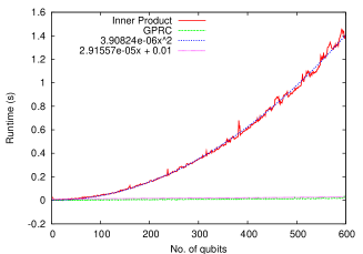
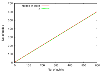
(a)	(b)

Figure 6: (a) Runtime results and regressions for the inner product and $\mathbf{GPRC}$ on checking global-phase equivalence of states generated by a Grover iteration. (b) Size in node count and regression of the QuIDD state vector.

Figure 6a shows the runtime results for the inner product and $\mathbf{GPRC}$ algorithms (no results are given for the node-count check algorithm since it runs in $O(1)$ time). The results confirm the asymptotic complexity differences between the algorithms. The number of nodes in the QuIDD state vector after a Grover iteration is $O(n)$ [25], which is confirmed in Figure 6b. As a result, the runtime complexity of the inner product should be $O(n^{2})$, which is confirmed by a regression plot within $1\%$ error. By contrast, the runtime complexity of the $\mathbf{GPRC}$ algorithm should be $O(n)$, which is also confirmed by another regression plot within $1\%$ error.

Figure 7a shows runtime results for the matrix product and $\mathbf{GPRC}$ algorithms checking the Grover operator. Like the state vector, it has been shown that the QuIDD for this operator grows in size as $O(n)$ [25], which is confirmed in Figure 7b. Therefore, the runtime of the matrix product should be quadratic in $n$ but linear in $n$ for $\mathbf{GPRC}$. Regression plots verify these complexities within $0.3\%$ error.

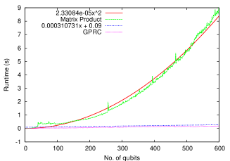
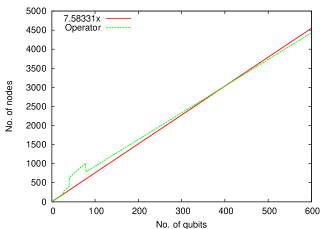
(a)	(b)

Figure 7: (a) Runtime results and regressions for the matrix product and $\mathbf{GPRC}$ on checking global-phase equivalence of the Grover iteration operator. (b) Size in node count and regression of the QuIDD representation of the operator.

The next benchmark compares states in Shor’s integer factorization algorithm [20]. Specifically, we consider states created by the modular exponentiation sub-circuit that represent all possible combinations of $x$ and $f(x,N)=a^{x}modN$, where $N$ is the integer to be factored [20] (see Figure 8). Each of the $O(2^{n})$ paths to a non-$0$ terminal represents a binary value for $x$ and $f(x,N)$. Thus, this benchmark tests performance with exponentially-growing QuIDDs.

${\scriptstyle x}\left[\begin{array}[]{l}\\ \\ \\ \\ \\ \\ \end{array}\right.$ ${\scriptstyle 7^{x}mod15}\left[\begin{array}[]{l}\\ \\ \\ \\ \\ \\ \end{array}\right.$

Figure 8: A QuIDD state combining $x$ and $7^{x}mod15$ in binary. The first qubit of each partition is least-significant.

Tables 1a-d show the results of the inner product and $\mathbf{GPRC}$ for this benchmark. Each $N$ is an integer whose two non-trivial factors are prime. $a$ is set to $N-2$ since it may be chosen randomly from the range $[2..N-2]$. In the case of Table 1a, states $\left|{\psi}\right\rangle$ and $\left|{\varphi}\right\rangle$ are equal up to global phase. The node counts for both states are equal as predicted by Lemma 2. Interestingly, both algorithms exhibit nearly the same performance. Tables 1b, 1c and 1d contain results for the cases in which Hadamard gates are applied to the first, middle, and last qubits, respectively, of $\left|{\varphi}\right\rangle$. The results show that early termination in $\mathbf{GPRC}$ can enhance performance by factors of roughly 1.5x to 10x.

No. of Creation No. of No. of Inner Product GPRC Qubits N Time (s) Nodes $\left|{\psi}\right\rangle$ Nodes $\left|{\varphi}\right\rangle$ Runtime (s) Runtime (s) $12$ $4031$ $11.9$ $9391$ $9391$ $0.30$ $0.26$ $13$ $6973$ $24.8$ $10680$ $10680$ $0.34$ $0.28$ $14$ $12127$ $55.1$ $18236$ $18236$ $0.54$ $0.46$ $15$ $19093$ $128.3$ $12766$ $12766$ $0.41$ $0.32$ $16$ $50501$ $934.1$ $51326$ $51326$ $1.7$ $1.6$ $17$ $69707$ $1969$ $26417$ $26417$ $0.87$ $0.78$ $18$ $163507$ $12788$ $458064$ $458064$ $19.6$ $19.6$ $19$ $387929$ $93547$ $182579$ $182579$ $6.62$ $6.02$	No. of Inner Product GPRC Nodes $\left|{\varphi}\right\rangle$ Runtime (s) Runtime (s) $10969$ $0.27$ $0.036$ $11649$ $0.31$ $0.036$ $19978$ $0.54$ $0.06$ $13446$ $0.41$ $0.036$ $55447$ $1.53$ $0.2$ $27797$ $0.78$ $0.084$ $521725$ $19.0$ $9.18$ $194964$ $6.44$ $4.40$
(a)	(b)
No. of Creation No. of No. of Inner Product GPRC Qubits N Time (s) Nodes $\left|{\psi}\right\rangle$ Nodes $\left|{\varphi}\right\rangle$ Runtime (s) Runtime (s) $12$ $4031$ $11.9$ $9391$ $11773$ $0.27$ $0.076$ $13$ $6973$ $24.8$ $10680$ $16431$ $0.43$ $0.14$ $14$ $12127$ $55.1$ $18236$ $29584$ $0.65$ $0.22$ $15$ $19093$ $128.3$ $12766$ $19207$ $0.56$ $0.20$ $16$ $50501$ $934.1$ $51326$ $71062$ $1.76$ $0.84$ $17$ $69707$ $1969$ $26417$ $46942$ $1.24$ $0.55$ $18$ $163507$ $12788$ $458064$ $653048$ $31.7$ $26.1$ $19$ $387929$ $93547$ $182579$ $312626$ $9.33$ $6.44$	No. of Inner Product GPRC Nodes $\left|{\varphi}\right\rangle$ Runtime (s) Runtime (s) $14092$ $0.21$ $0.088$ $16431$ $0.27$ $0.084$ $29584$ $0.53$ $0.13$ $19207$ $0.50$ $0.084$ $74919$ $1.51$ $0.66$ $46942$ $1.13$ $0.25$ $629533$ $29.6$ $23.7$ $312626$ $13.0$ $8.62$
(c)	(d)

Table 1: Performance results for the inner product and $\mathbf{GPRC}$ algorithms on checking global-phase equivalence of modular exponentiation states. In (a), $\left|{\psi}\right\rangle=\left|{\varphi}\right\rangle$ up to global phase. In (b), (c), and (d), Hadamard gates are applied to the first, middle, and last qubits, respectively, of $\left|{\varphi}\right\rangle$ so that $\left|{\psi}\right\rangle\neq\left|{\varphi}\right\rangle$ up to global phase.

In almost every case, both algorithms represent far less than $1\%$ of the total runtime. Thus, checking for global-phase equivalence among QuIDD states appears to be an easily achievable task once the representations are created. An interesting side note is that some modular exponentiation QuIDD states with more qubits can have more exploitable structure than those with fewer qubits. For instance, the $N=387929$ ($19$ qubits) QuIDD has fewer than half the nodes of the $N=163507$ ($18$ qubits) QuIDD.

Table 2 contains results for the matrix product and $\mathbf{GPRC}$ algorithm checking the inverse Quantum Fourier Transform (QFT) operator. The inverse QFT is a key operator in Shor’s algorithm [20], and it has been previously shown that its $n$-qubit QuIDD representation grows as $O(2^{2n})$ [25]. In this case, the asymptotic differences in the matrix product and $\mathbf{GPRC}$ are very noticeable. Also, the memory usage indicates that the matrix product may need asymptotically more intermediate memory despite operating on QuIDDs with the same number of nodes as $\mathbf{GPRC}$.

No. of	Matrix Product		GPRC
Qubits	Time (s)	Mem (MB)	Time (s)	Mem (MB)
5	2.53	1.41	0.064	0.25
6	22.55	6.90	0.24	0.66
7	271.62	46.14	0.98	2.03
8	3637.14	306.69	4.97	7.02
9	22717	1800.42	17.19	26.48
10	—	$>2GB$	75.38	102.4
11	—	$>2GB$	401.34	403.9

Table 2: Performance results for the matrix product and $\mathbf{GPRC}$ algorithms on checking global-phase equivalence of the QFT operator used in Shor’s factoring algorithm. $>2GB$ indicates that a memory usage cutoff of 2GB was exceeded.

4 Checking Equivalence up to Relative Phase

The relative-phase checking problem can also be solved in many ways. The first three algorithms are adapted from linear algebra to QuIDDs, while the last two exploit DD properties directly, offering asymptotic improvements.

4.1 Modulus and Inner Product

Consider two state vectors $\left|{\psi}\right\rangle$ and $\left|{\varphi}\right\rangle$ that are equal up to relative phase and have complex-valued elements $w_{j}$ and $v_{k}$, respectively, where $j,k=0,1,\ldots,N-1$. Computing $\left|{\varphi^{\prime}}\right\rangle=\Sigma_{i=0}^{N-1}|v_{j}|\left|{j}\right\rangle$ and $\left|{\psi^{\prime}}\right\rangle=\Sigma_{k=0}^{N-1}|w_{k}|\left|{k}\right\rangle=\Sigma_{k=0}^{N-1}|e^{i\theta_{k}}v_{k}|\left|{k}\right\rangle$ sets each phase factor to a $1$, allowing the inner product to be applied as in Subsection 3.1. The complex modulus operations are computed as $C=\mathbf{Apply}(A,|\cdot|)$ and $D=\mathbf{Apply}(B,|\cdot|)$ with runtime and memory complexity $O(|A|+|B|)$, which is dominated by the $O(|A||B|)$ inner product complexity.

4.2 Modulus and Matrix Product

For operator equivalence up to relative phase, two cases are considered, namely the diagonal relative-phase matrix appearing on the left or right side of one of the operators. Consider two operators $U$ and $V$ with elements $u_{j,k}$ and $v_{j,k}$, respectively, where $j,k=0,\ldots N-1$. The two cases in which the relative-phase factors appear on either side of $V$ are described as $u_{j,k}=e^{i\theta_{j}}v_{j,k}$ (left side) and $u_{j,k}=e^{i\theta_{k}}v_{j,k}$ (right side). In either case the the matrix product check discussed in Subsection 3.2 may be extended by computing the complex modulus without increasing the overall complexity. Note that neither this algorithm nor the modulus and inner product algorithm calculate the relative-phase factors.

4.3 Element-wise Division

Given the states discussed in Subsection 4.1, $w_{k}=e^{i\theta_{k}}v_{k}$, the operation $w_{k}/v_{j}$ for each $j=k$ is a relative-phase factor, $e^{i\theta_{k}}$. The condition $|w_{k}/v_{j}|=1$ is used to check if each division yields a relative phase. If this condition is satisfied for all divisions, the states are equal up to relative phase.

The QuIDD implementation for states is simply $C=\mathbf{Apply}(A,B,/)$, where $\mathbf{Apply}$ is augmented to avoid division by $0$ and instead return $1$ when two terminal values being compared equal $0$ and return $0$ otherwise. $\mathbf{Apply}$ can be further augmented to terminate early when $|w_{j}/v_{i}|\neq 1$. $C$ is a QuIDD vector containing the relative-phase factors. If $C$ contains a terminal value of $0$, then $A$ and $B$ do not differ by relative phase. Since a call to $\mathbf{Apply}$ implements this algorithm, the runtime and memory complexity are $O(|A||B|)$.

Element-wise division for operators is more complicated. For QuIDD operators $U$ and $V$, $W=\mathbf{Apply}(U,V,/)$ is a QuIDD matrix with the relative-phase factor $e^{i\theta_{j}}$ along row $j$ in the case of phases appearing on the left side and along column $j$ in the case of phases appearing on the right side. In the first case, all rows of $W$ are identical, meaning that the support of $W$ does not contain any row variables. Similarly, in the second case the support of $W$ does not contain any column variables. A complication arises when $0$ values appear in either operator. In such cases, the support of $W$ may contain both variable types, but the operators may in fact be equal up to relative phase. Figure 9 presents an algorithm based on $\mathbf{Apply}$ which accounts for these special cases by using a sentinel value of $2$ to mark valid $0$ entries that do not affect relative-phase equivalence. These entries are recursively ignored by skipping either row or column variables with sentinel children ($S$ specifies row or column variables), which effectively fills copies of neighboring row or column phase values in their place in $W$. The algorithm must be run twice, once for each variable type. The size of $W$ is $O(|U||V|)$ since it is created with a variant of $\mathbf{Apply}$.

$\begin{array}[]{l}\mathbf{RP\_DIV}(A,B,S)\ \{\\ \hskip 8.00002pt\mathbf{if}\ (A\ ==\ New\_Terminal(0))\ \{\\ \hskip 16.00003pt\mathbf{if}\ (B\ !=\ New\_Terminal(0))\\ \hskip 24.00005pt\mathbf{return}\ New\_Terminal(0);\\ \hskip 16.00003pt\mathbf{return}\ New\_Terminal(2);\\ \hskip 8.00002pt\}\\ \hskip 8.00002pt\mathbf{if}\ (Is\_Constant(A)\ \mathbf{and}\ Is\_Constant(B))\ \{\\ \hskip 16.00003ptnrp=Value(A)/Value(B);\\ \hskip 16.00003pt\mathbf{if}\ (\mathbf{sqrt}(\mathbf{real}(nrp)*\mathbf{real}(nrp)+\\ \hskip 24.00005pt\mathbf{imag}(nrp)*\mathbf{imag}(nrp))\ !=\ 1)\\ \hskip 32.00006pt\mathbf{return}\ New\_Terminal(0);\\ \hskip 16.00003pt\mathbf{return}\ New\_Terminal(nrp);\\ \hskip 8.00002pt\}\\ \hskip 8.00002pt\mathbf{if}\ (Table\_Lookup(R,RP\_DIV,A,B,S))\ \mathbf{return}\ R;\\ \hskip 8.00002ptv\ =\ Top\_Var(A,B);\\ \hskip 8.00002ptT\ =\ \mathbf{RP\_DIV}(A_{v},B_{v},S);\\ \hskip 8.00002ptE\ =\ \mathbf{RP\_DIV}(A_{v^{\prime}},B_{v^{\prime}},S);\\ \hskip 8.00002pt\mathbf{if}\ ((T\ ==\ New\_Terminal(0))\ \mathbf{or}\\ \hskip 16.00003pt(E\ ==\ New\_Terminal(0)))\\ \hskip 24.00005pt\mathbf{return}\ New\_Terminal(0);\\ \hskip 8.00002pt\mathbf{if}\ ((T\ !=\ E)\ \mathbf{and}\ (Type(v)\ ==\ S))\ \{\\ \hskip 16.00003pt\mathbf{if}\ (Is\_Constant(T)\ \mathbf{and}\ Value(T)\ ==\ 2)\\ \hskip 24.00005pt\mathbf{return}\ E;\\ \hskip 16.00003pt\mathbf{if}\ (Is\_Constant(E)\ \mathbf{and}\ Value(E)\ ==\ 2)\\ \hskip 24.00005pt\mathbf{return}\ T;\\ \hskip 16.00003pt\mathbf{return}\ New\_Terminal(0);\\ \hskip 8.00002pt\}\\ \hskip 8.00002pt\mathbf{if}\ (Is\_Constant(T)\ \mathbf{and}\ Value(T)\ ==\ 2)\\ \hskip 16.00003ptT\ =\ New\_Terminal(1);\\ \hskip 8.00002pt\mathbf{if}\ (Is\_Constant(E)\ \mathbf{and}\ Value(E)\ ==\ 2)\\ \hskip 16.00003ptE\ =\ New\_Terminal(1);\\ \hskip 8.00002ptR\ =\ \mathbf{ITE}(v,T,E);\\ \hskip 8.00002ptTable\_Insert(R,RP\_DIV,A,B,S);\\ \hskip 8.00002pt\mathbf{return}\ R;\\ \}\end{array}$

Figure 9: Element-wise division algorithm.

4.4 Non-0 Terminal Merge

A necessary condition for relative-phase equivalence is that zero-valued elements of each state vector appear in the same locations, as expressed by the following lemma.

Lemma 3

A necessary but not sufficient condition for two states $\left|{\varphi}\right\rangle=\Sigma_{j=0}^{N-1}v_{j}\left|{j}\right\rangle$ and $\left|{\psi}\right\rangle=\Sigma_{k=0}^{N-1}w_{k}\left|{k}\right\rangle$ to be equal up to relative phase is that $\forall v_{j}=w_{k}=0$, $j=k$.

Proof. If $\left|{\psi}\right\rangle=\left|{\varphi}\right\rangle$ up to relative phase, $\left|{\psi}\right\rangle=\Sigma_{k=0}^{N-1}e^{i\theta_{k}}v_{k}\left|{k}\right\rangle$. Since $e^{i\theta_{k}}\neq 0$ for any $\theta$, if any $w_{k}=0$, then $v_{j}=0$ must also be true where $j=k$. A counter-example proving insufficiency is $\left|{\psi}\right\rangle=(0,1/\sqrt{3},1/\sqrt{3},1/\sqrt{3})^{T}$ and $\left|{\varphi}\right\rangle=(0,1/2,1/\sqrt{2},1/2)^{T}$. $\Box$

QuIDD canonicity may now be exploited. Let $A$ and $B$ be the QuIDD representations of the states $\left|{\psi}\right\rangle$ and $\left|{\varphi}\right\rangle$, respectively. First compute $C=\mathbf{Apply}(A,\lceil|\cdot|\rceil)$ and $D=\mathbf{Apply}(B,\lceil|\cdot|\rceil)$, which converts every non-zero terminal value of $A$ and $B$ into a $1$. Since $C$ and $D$ have only two terminal values, $0$ and $1$, checking if $C=D$ satisfies Lemma 3. Canonicity ensures this check requires $O(1)$ time and memory. The overall runtime and memory complexity of this algorithm is $O(|A|+|B|)$ due to the unary $\mathbf{Apply}$ operations. This algorithm also applies to operators since Lemma 3 also applies to $u_{j,k}=e^{i\theta_{j}}v_{j,k}$ (phases on the left) and $u_{j,k}=e^{i\theta_{k}}v_{j,k}$ (phases on the right) for operators $U$ and $V$.

4.5 Modulus and DD Compare

A variant of the algorithm presented in Subsection 4.1, which also exploits canonicity, provides an asymptotic improvement for checking a necessary and sufficient condition of relative-phase equivalence of states and operators. As in Subsection 4.1, compute $C=\mathbf{Apply}(A,|\cdot|)$ and $D=\mathbf{Apply}(B,|\cdot|)$. If $A$ and $B$ are equal up to relative phase, then $C=D$ since each phase factor becomes a $1$. This check requires $O(1)$ time and memory due to canonicity. Thus, the runtime and memory complexity is dominated by the unary $\mathbf{Apply}$ operations, giving $O(|A|+|B|)$.

4.6 Empirical Results for Relative-Phase
Equivalence Algorithms

The first benchmark for the relative-phase equivalence checking algorithms creates a remote EPR pair, which is an EPR pair between the first and last qubits, via nearest-neighbor interactions [7]. The circuit is shown in Figure 10. Specifically, it transforms the initial state $\left|{00\ldots 0}\right\rangle$ into $(1/\sqrt{2})(\left|{00\ldots 0}\right\rangle+\left|{10\ldots 1}\right\rangle)$. The circuit size is varied, and the final state is compared to the state $(e^{0.345i}/\sqrt{2})\left|{00\ldots 0}\right\rangle+(e^{0.457i}/\sqrt{2})\left|{10\ldots 1}\right\rangle$.

Figure 10: Remote EPR-pair creation between the first and last qubits via nearest-neighbor interactions.

The results in Figure 11a show that all algorithms run quickly. The inner product is the slowest, yet it runs in approximately 0.2 seconds at $1000$ qubits, a small fraction of the 7.6 seconds required to create the QuIDD state vectors. Regressions of the runtime and memory data reveal linear complexity for all algorithms to within $1\%$ error. This is not unexpected since the QuIDD representations of the states grow linearly with the number of qubits (see Figure 11b), and the complex modulus reduces the number of different terminals prior to computing the inner product. These results illustrate that in practice, the inner product and element-wise division algorithms can perform better than their worst-case complexity. Element-wise division should be preferred when QuIDD states are compact since unlike the other algorithms, it computes the relative-phase factors.

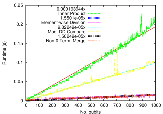
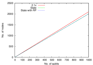
(a)	(b)

Figure 11: (a) Runtime results and (b) size in nodes plotted with regressions for inner product, element-wise division, modulus and DD compare, and non-$0$ terminal merge checking relative-phase equivalence of the remote EPR pair circuit.

Figure 12: A quantum-circuit realization of a Hamiltonian consisting of Pauli operators.

The Hamiltonian simulation circuit shown in Figure 12 is taken from [15, Figure 4.19, p. 210]. When its one-qubit gate (boxed) varies with $\Delta t$, it produces a variety of diagonal operators, all of which are equivalent up to relative phase. Empirical results for such equivalence checking are shown in Figure 13. As before, the matrix product and element-wise division algorithms perform better than their worst-case bounds, indicating that element-wise division is the best choice for compact QuIDDs.

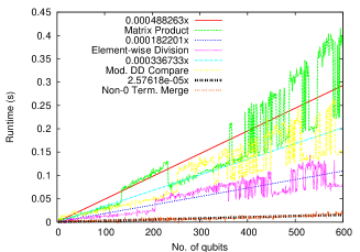
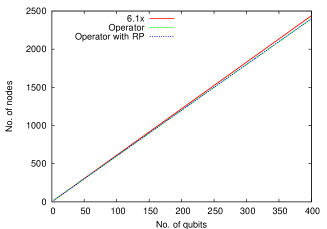
(a)	(b)

Figure 13: (a) Runtime results and (b) size in nodes plotted with regressions for matrix product, element-wise division, modulus and DD compare, and non-$0$ terminal merge checking relative-phase equivalence of the Hamiltonian $\Delta t$ circuit.

5 Conclusions

Although DD properties like canonicity enable exact equivalence checking in $O(1)$ time, we have shown that such properties may be exploited to develop efficient algorithms for the difficult problem of equivalence checking up to global and relative phase. In particular, the global-phase recursive check and element-wise division algorithms efficiently determine equivalence of states and operators up to global and relative phase, and compute the phases. In practice, they outperform QuIDD matrix and inner products, which do not compute relative-phase factors. Other QuIDD algorithms presented in this work, such as the node-count check, non-$0$ terminal merge, and modulus and DD compare, exploit other DD properties to provide even faster checks but only satisfy necessary equivalence conditions. Thus, they should be used to aid the more robust algorithms. A summary of the theoretical results is provided in Table 3.

				$O(\cdot)$ time	$O(\cdot)$ time
Algorithm	Phase	Finds	Necessary &	complexity:	complexity:
	type	phases?	sufficient?	best-case	worst-case
Inner
Product	Global	Yes	N. & S.	$|A||B|$	$|A||B|$
Matrix
Product	Global	Yes	N. & S.	$(|A||B|)^{2}$	$(|A||B|)^{2}$
Node-Count	Global	No	N. only	$1$	$1$
Recursive
Check	Global	Yes	N. & S.	$\mathbf{1}$	$\mathbf{|A|+|B|}$
Modulus and
Inner Product	Relative	No	N. & S.	$|A||B|$	$|A||B|$
Element-wise
Division	Relative	Yes	N. & S.	$\mathbf{|A||B|}$	$\mathbf{|A||B|}$
Non-$0$
Terminal Merge	Relative	No	N. only	$|A|+|B|$	$|A|+|B|$
Modulus and
DD Compare	Relative	No	N. & S.	$|A|+|B|$	$|A|+|B|$

Table 3: Key properties of the QuIDD-based phase-equivalence checking algorithms.

The algorithms presented here enable QuIDDs and other DD datastructures to be used in synthesis and verification of quantum circuits. A fair amount of work has been done on optimal synthesis for small quantum circuits as well as heuristics for larger circuits via circuit transformations [16, 18]. Equivalence checking in particular plays a key role in some of these techniques since it is often necessary to verify the correctness of the transformations. Future work will determine how these equivalence checking algorithms may be used as primitives to enhance such heuristics.

Acknowledgements. This work was funded by the Air Force Research Laboratory. The views and conclusions contained herein are those of the authors and should not be interpreted as necessarily representing official policies or endorsements of employers and funding agencies.

References

- [1]
- [2] S. Aaronson and D. Gottesman, “Improved simulation of stabilizer circuits”, Phys. Rev. A, 70, 052328, 2004.
- [3] R. I. Bahar et al., “Algebraic decision diagrams and their applications,” Journal of Formal Methods in System Design, 10 (2/3), 1997.
- [4] A. Barenco et al., “Elementary gates for quantum computation,” Phys. Rev. A, 52, 3457-3467, 1995.
- [5] C. H. Bennett and G. Brassard, “Quantum cryptography: public key distribution and coin tossing”, In Proc. of IEEE Intl. Conf. on Computers, Systems, and Signal Processing, pp. 175-179, 1984.
- [6] C.H. Bennett, “Quantum cryptography using any two nonorthogonal states”, Phys. Rev. Lett. 68, 3121, 1992.
- [7] G. P. Berman, G. V. López, and V. I. Tsifrinovich, “Teleportation in a nuclear spin quantum computer,” Phys. Rev. A 66, 042312, 2002.
- [8] R. Bryant, “Graph-based algorithms for Boolean function manipulation,” IEEE Trans. on Computers, C35, pp. 677-691, 1986.
- [9] E. Clarke et al., “Multi-terminal binary decision diagrams and hybrid decision diagrams,” in T. Sasao and M. Fujita, eds, Representations of Discrete Functions, pp. 93-108, Kluwer, 1996.
- [10] S. A. Cuccaro, T. G. Draper, S. A. Kutin, and D. P. Moulton, “A new quantum ripple-carry addition circuit,” quant-ph/0410184, 2004.
- [11] D. Gottesman, “The Heisenberg representation of quantum computers,” Plenary speech at the 1998 International Conference on Group Theoretic Methods in Physics, quant-ph/9807006, 1998.
- [12] L. Grover, “Quantum mechanics helps in searching for a needle in a haystack,” Phys. Rev. Lett. 79, 325, 1997.
- [13] A. J. G. Hey, ed., Feynman and Computation: Exploring the Limits of Computers, Perseus Books, 1999.
- [14] D. Maslov, S. M. Falconer, M. Mosca, “Quantum Circuit Placement: Optimizing Qubit-to-qubit Interactions through Mapping Quantum Circuits into a Physical Experiment,” to appear in DAC 2007, quant-ph/0703256.
- [15] M. A. Nielsen, I. L. Chuang, Quantum Computation and Quantum Information, Cambridge Univ. Press, 2000.
- [16] A. K. Prasad, V. V. Shende, K. N. Patel, I. L. Markov, and J. P. Hayes, “Algorithms and data structures for simplifying reversible circuits”, to appear in ACM J. of Emerging Technologies in Computing, 2007.
- [17] V. V. Shende, Personal communication, September 2006.
- [18] V. V. Shende, S. S. Bullock, I. L. Markov, “Synthesis of quantum logic circuits,” IEEE Trans. on CAD 25, pp. 1000-1010, 2006.
- [19] V. V. Shende and I. L. Markov, “Quantum circuits for incompletely specified two-qubit operators,” Quantum Information and Computation 5 (1), pp. 49-57, 2005.
- [20] P. W. Shor, “Polynomial-time algorithms for prime factorization and discrete logarithms on a quantum computer,” SIAM J. of Computing, 26, p. 1484, 1997.
- [21] G. Song and A. Klappenecker, “Optimal realizations of simplified Toffoli gates,” 4, pp. 361-372, 2004.
- [22] R. T. Stanion, D. Bhattacharya, and C. Sechen, “An efficient method for generating exhaustive test sets,” IEEE Trans. on CAD 14, pp. 1516-1525, 1995.
- [23] R. Van Meter and K. M. Itoh, “Fast quantum modular exponentiation,” Phys. Rev. A 71, 052320, 2005.
- [24] G. F. Viamontes, I. L. Markov, J. P. Hayes, “Graph-based simulation of quantum computation in the density matrix representation,” Quantum Information and Computation 5 (2), pp. 113-130, 2005.
- [25] G. F. Viamontes, I. L. Markov, and J. P. Hayes, “Improving gate-level simulation of quantum circuits,” Quantum Information Processing 2, pp. 347-380, 2003.
- [26] G. Vidal, “Efficient classical simulation of slightly entangled quantum computations,” Phys. Rev. Lett. 91, 147902, 2003.
- [27] J. Yepez, “A quantum lattice-gas model for computational fluid dynamics,” Phys. Rev. E 63, 046702, 2001.