An Analysis of the Shapes of Interstellar Extinction Curves. V. The IR-Through-UV Curve Morphology

Abstract

We study the IR-through-UV wavelength dependence of 328 Galactic interstellar extinction curves affecting normal, near-main sequence B and late O stars. We derive the curves using a new technique which employs stellar atmosphere models in lieu of unreddened “standard” stars. Under ideal conditions, this technique is capable of virtually eliminating spectral mismatch errors in the curves. In general, it lends itself to a quantitative assessment of the errors and enables a rigorous testing of the significance of relationships between various curve parameters, regardless of whether their uncertainties are correlated. Analysis of the curves gives the following results:

1. In accord with our previous findings, the central position of the 2175 Å extinction bump is mildly variable, its width is highly variable, and the two variations are unrelated.

2. Strong correlations are found among some extinction properties within the UV region, and within the IR region.

3. With the exception of a few curves with extreme (i.e., large) values of $R(V)$, the UV and IR portions of Galactic extinction curves are not correlated with each other.

4. The large sightline-to-sightline variation seen in our sample implies that any average Galactic extinction curve will always reflect the biases of its parent sample.

5. The use of an average curve to deredden a spectral energy distribution (SED) will result in significant errors, and a realistic error budget for the dereddened SED must include the observed variance of Galactic curves.

While the observed large sightline-to-sightline variations, and the lack of correlation among the various features of the curves, make it difficult to meaningfully characterize average extinction properties, they demonstrate that extinction curves respond sensitively to local conditions. Thus, each curve contains potentially unique information about the grains along its sightline.

1 INTRODUCTION

In the previous paper in this series (Fitzpatrick & Massa 2005a, hereafter Paper IV), we introduced a technique, “extinction-without-standards,” to determine the shapes of UV-through-IR interstellar extinction curves by modeling the observed spectral energy distributions (SEDs) of reddened early-type stars. The method involves a $\chi^{2}$-minimization procedure to determine simultaneously the basic properties of a reddened star (namely, $T_{\rm eff}$, $\log g$, [m/H], and $v_{turb}$) and the shape of its extinction curve, utilizing grids of stellar atmosphere models to represent intrinsic SEDs and an analytical form of the extinction curve, whose shape is determined by a set of adjustable parameters.

In general, the benefits of extinction-without-standards are increased accuracy and precision (in most applications) over results generated using the standard Pair Method of extinction curve determination and, very importantly, a reliable estimate of the uncertainties in the resultant extinction curves. Specifically, the advantages of the new method include: (1) the elimination of the requirement for observations of unreddened spectral standard stars, (2) the near-elimination of “spectral mismatch” as a source of extinction curve error, (3) the ability to produce accurate curves for much more lightly-reddened sightlines than heretofore possible, (4) the ability to derive accurate ultraviolet curves for later spectral types (i.e., to late-B classes) than previously possible, and (5) the ability to provide quantified estimates of the degree of correlation between various morphological features of the curves.

The chief limitation of the method is that the intrinsic SEDs of the reddened stars must be well-represented by model atmosphere calculations. This currently eliminates from consideration such objects as high luminosity stars, Be stars, Wolf-Rayet stars, and any spectrally peculiar star. This restriction also affects the Pair Method, since there are only a small number of unreddened members of these classes which can serve as “standard stars,” and it is difficult to be certain that the intrinsic SEDs of the standard stars really represent those of the reddened stars. In addition, the extinction-without-standards technique requires well-calibrated (and absolutely-calibrated) SED observations.

In this paper, we apply our extinction-without-standards technique to a sample of 328 Galactic stars for which multi-wavelength SEDs are available. For these stars, we derive normalized UV-through-IR extinction curves, sets of parameters which describe the shapes of the curves, and sets of parameters which characterize the stars themselves. The scope of our discussion focuses on two objectives: (1) the presentation of the broad-ranging results and a description of the methodology employed, and (2) a thorough examination of general extinction curve morphology. Among the issues addressed is the correlation between the IR and UV properties of extinction (see, e.g., Cardelli, Clayton, & Mathis 1989). This paper is not intended as a review of Galactic extinction and we explicitly restrict our attention only to issues touched upon by our new analysis. The results, however, do constitute a broad view of Galactic extinction and lend themselves to numerous other investigations, including the general properties of extinction curves, regional trends in extinction properties, the correlation between extinction and other interstellar properties, determination of intrinsic SEDs for objects in clusters containing survey stars, the study of small scale spatial variations in dust grain populations from stars in cluster extinction curves, etc. We plan to pursue some of these in future papers. Preliminary results from an early version of this study were reported by Fitzpatrick (2004; hereafter F04), which also provided a review of then-recent progress in interstellar extinction studies.

The sample of stars chosen for this survey and the data used are described in §2. This is followed in §3 by a brief description of the extinction-without-curves technique, including a discussion of the error analysis — which is critical to the analyses in the latter parts of the paper. The results of the survey, essentially an atlas of Galactic extinction curves, is presented in §4, with the full sets of tables and the full set of figures from this section available in the electronic edition of the Journal. In §5 we briefly discuss the stellar properties derived from our analysis and then in §6 present a detailed description of Galactic extinction curve morphology, from the IR to the UV spectral regions. Finally, in §7 we provide a brief summary of the chief conclusions of this study.

2 THE SURVEY STARS AND THEIR DATA

In principle, the extinction-without-standards technique can be applied to, or expanded to include, any type of SED data. In practice, however, we have developed the technique with specific datasets in mind, namely, low-resolution UV spectrophotometry from the International Ultraviolet Explorer (IUE) satellite and ground-based optical and near-IR photometry. In this particular study, we utilize IUE spectrophotometry, UBV photometry, and JHK photometry from the Two-Micron All Sky Survey (2MASS). Although some of the survey stars have additional data available, e.g., Strömgren $uvby\beta$ photometry, we elected — for the sake of uniformity — to include only the UBV data in the analysis. As a result, the stellar parameters we derive in this paper will be less accurate than those determined in Paper IV. Nevertheless, the errors in these parameters are still well-determined.

The most restrictive of the datasets is that of the IUE, and so we began our search for survey stars with the IUE database. Using the search engine provided by the Multimission Archive at STScI (MAST), we examined all low-resolution spectra for stars with IUE Object Class numbers of 12 (main sequence O), 20 (B0-B2 V-IV), 21 (B3-B5 V-IV), 22 (B6-B9.5 V-IV), 23 (B0-B2 III-I), 24 (B3-B5 III-I), and 25 (B6-B9.5 III-I). Because our goal is to obtain a uniform dataset of reddened stars whose SEDs can be modeled accurately, we eliminated the following types of objects from the available field of candidates: (1) stars without good-quality spectra from both the short-wavelength (SWP) and long-wavelength (LWR or LWP) IUE spectral regions, (2) clearly-unreddened stars, (3) known Be stars, (4) luminosity class I stars, (5) O stars more luminous than class V, (6) O stars earlier than spectral type O5, and (7) stars with peculiar-looking UV spectra (as based on our own assessment).

The list of potential candidates from the IUE database was then examined for the availability of UBV data, using the General Catalog of Photometric Data (GCPD) maintained at the University of Geneva (see Mermilliod, Mermilliod, & Hauck 1997). In general, stars without V and B V measurements were eliminated from consideration. However, broadband Geneva photometry was available for five stars without UBV data (BD+56 526, HD62542, HD108927, HD110336, and HD143054), and so we included these stars and utilized the Geneva $U-B$ and $V-B$ indices.

The final trimming of the survey sample was not performed until the SEDs had been modeled. At this point we imposed the requirement that all survey stars must have values of $\mbox{$E(B\!-\!V)$}\geq 0.20$ mag. This limit is somewhat arbitrary and, as shown by Paper IV, useful extinction curves can be derived via the extinction-without-standards technique for $E(B\!-\!V)$ values considerably lower than 0.20 mag. However, the uncertainties do rise at low $E(B\!-\!V)$ and for this survey we wanted a sample of stars for which the uncertainties in the final parameters were uniformly small. We plan in the future to examine the extinction properties along lightly reddened sightlines.

Near-IR JHK photometry (and their associated uncertainties) were retrieved for the survey stars from the 2MASS database at the NASA/IPAC Infrared Science Archive (IRSA). Only those 2MASS magnitudes for which the uncertainties are less than $\pm 0.1$ mag are used here. For seven stars whose 2MASS measurements were either non-existent or of low quality (HD23180, HD23512, HD37022, HD144470, HD147165, HD147933, and HD149757), Johnson JHK magnitudes were available and were retrieved via the GCPD catalog. Note that the availability of JHK data was not a requirement for inclusion in this survey although, as will be quantified below, most of our sample have such data.

The last data collection activity was to retrieve ancillary information for all stars, such as coordinates, alternate names, and spectral types, using the SIMBAD database.

The only data processing required for this program involved the IUE spectrophotometry. The IUE data contained in the MAST archive were processed using the NEWSIPS software (Nichols & Linsky 1996). As discussed in detail by Massa and Fitzpatrick (2000; hereafter MF00), these data contain significant thermal and temporal dependencies and suffer from an incorrect absolute calibration. We corrected the data for their systematic errors and placed them onto the HST/FOS flux scale of Bohlin (1996) using the corrections and algorithms described and provided by MF00. This step is absolutely essential for our program since our “comparison stars” for deriving extinction curves are stellar atmosphere models and systematic errors in the absolute calibration of the data do not cancel out as they would in the case of the Pair Method. (Note that the thermally- and temporally-dependent errors in the NEWSIPS data would not generally cancel out in the Pair Method — see MF00.) When multiple spectra were available in one of IUE’s wavelength ranges (SWP or LWR and LWP), they were combined using the NEWSIPS error arrays as weights. Small aperture data were scaled to the large aperture data and both trailed and point source data were included. Short and long wavelength data were joined at 1978 Å to form a complete spectrum covering the wavelength range $1150\leq\lambda\leq 3000$ Å. Data longward of 3000 Å were ignored because they are typically of low quality and subject to residual systematic effects.

After all the limits and restrictions were imposed, we arrived at our final sample of 328 stars for which UV spectrophotometry covering 1150-3000 Å and UBV photometry are available. Of these, 298 stars have at least some near-IR photometry, while 287 have a complete set of J-, H-, and K- band measurements (with 280 of these from the 2MASS program). Table An Analysis of the Shapes of Interstellar Extinction Curves. V. The IR-Through-UV Curve Morphology lists all the survey stars, along with some general descriptive information. (The complete version of Table An Analysis of the Shapes of Interstellar Extinction Curves. V. The IR-Through-UV Curve Morphology appears in the electronic version of the paper.) The stars in Table 1 are ordered by Right Ascension. For the star names, we adopted the most common form among all the possibilities listed in the SIMBAD database (i.e., “HDnnn” was the most preferred, followed by “BDnnn”, etc.) There are 185 survey stars which are members of open clusters or associations. The identity of the cluster or association is either contained in the star name itself (e.g., NGC 457 Pesch 34) or is given in parentheses after the star’s name. The spectral types in Table An Analysis of the Shapes of Interstellar Extinction Curves. V. The IR-Through-UV Curve Morphology were selected from those given in the SIMBAD database, and the source of the adopted types is shown in the “Reference” column of the table. When multiple types were available for a particular star, we selected one based on our own preferred ranking of the sources. For the B stars, the quality of the spectral types varies widely, and the types themselves are given only as a general reference — they do not play any role in our analysis. A scan of the types seems to indicate that in some instances we have violated our selection criteria, e.g., several “Ib”s and “e”s can be found. However, in our estimation, these are unreliable types and do not reflect the spectral information we have examined. For example, a number of B stars in clusters have been erroneously classified as emission-line stars based on contamination of their spectra by nebular emission lines. The O stars in the sample are, on the other hand, uniformly well-classified and the types are used in the analysis (see §4).

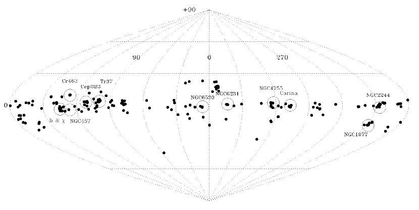
Figure 1: Sky distribution of survey stars, shown in a sinusoidal projection of Galactic coordinates. The Galactic plane is the solid horizontal line and the Galactic center is in the middle of the figure. The locations of open clusters or associations containing five or more survey stars are indicated by the large circles, labeled with the cluster name. The sizes of the circles do not represent the physical extent of the clusters or associations.

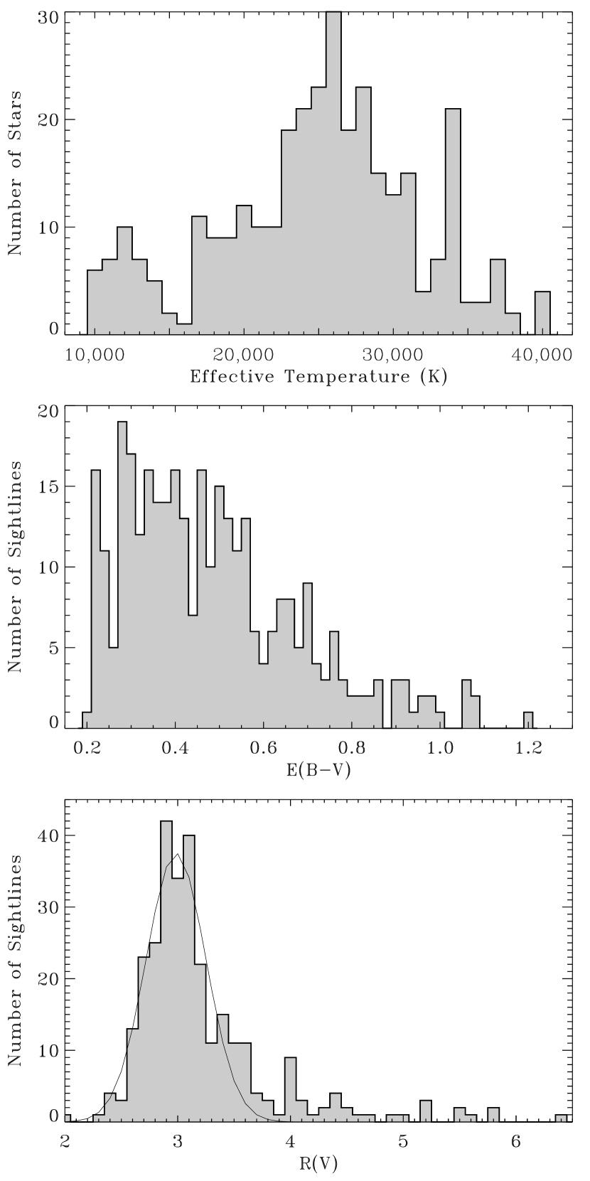
Figure 2: Representative properties of the survey stars. The three panels show results from the analysis presented in §4, which help characterize the properties of our sample. The typical survey member is a mid-B star (top panel), with a median reddening of $\overline{\mbox{$E(B\!-\!V)$}}=0.45$ mag (middle panel), viewed along a line-of-sight passing through the diffuse ISM (bottom panel). The bottom panel also shows a Gaussian fit to the values of $R(V)\equiv A_{V}/\mbox{$E(B\!-\!V)$}$ in the neighborhood of the peak in the distribution. The peak is located at $R(V)=2.99$, similar to the mean values usually attributed to the diffuse ISM, and the width of the Gaussian corresponds to $\sigma=\pm 0.27$. The mean and median values of $R(V)$ for the whole sample are 3.22 and 3.05, respectively.

An overview of the survey sample can be gained from Figures 1 and 2. The former shows the location of the stars on the sky (in Galactic coordinates) and the latter summarizes the breadth of the stellar and interstellar properties of the sample. Figure 1 shows that our sample is clearly biased to sightlines passing through the galactic plane, as would be expected given by the lower limit of $\mbox{$E(B\!-\!V)$}=0.20$ mag which we imposed. The locations of open clusters or associations for which five of more members are in the survey sample are indicated on the figure by the large circles. Note that the size of the circles is not intended to represent the physical extent of the clusters or associations. The data shown in histogram form in Figure 2 are final results from the analysis, but are useful here to characterize the sample. Most of our stars are mid-to-early B stars ($\mbox{$T_{\rm eff}$}=15000-30000$ K) with a median reddening of $\mbox{$E(B\!-\!V)$}=0.45$ mag. The median value of $R(V)$ ($\equiv A_{V}/\mbox{$E(B\!-\!V)$}$) for the sample is 3.05, essentially identical to the Galactic mean value for the diffuse ISM, and our sample is dominated by sightlines though the diffuse ISM. However — due to the relatively small sample size and the biases present in the IUE satellite’s choice of targets over the years — our survey does not necessarily constitute a representative sample of the various types of regions present in the ISM. Care must be taken in interpreting average properties derived from our results.

3 THE ANALYSIS

It was shown by Paper IV that the energy distributions of reddened B-type stars could be modeled successfully using theoretical predictions of the intrinsic SEDs of the stars and a parametrized form of the UV-through-IR extinction curve to account for the distortions introduced by interstellar extinction. A byproduct of the fit is a determination of the wavelength-dependence of the extinction affecting the star. This is the essence of the extinction-without-standards technique. Although it was discussed in detail by Paper IV, for completeness, we use this section to outline the basics of the technique. In addition, some details of the process have changed since Paper IV, as a result of experience gained from the application of the process to several hundred reddened stars. These changes are highlighted here.

3.1 Modeling the SEDs

The observed SED $f_{\lambda}$ of a reddened star can be represented as

$$f_{\lambda}=F_{\lambda}\,\theta_{R}^{2}\,10^{-0.4E(B-V)[k(\lambda-V)+R(V)]}\;\;,$$ (1)

where $F_{\lambda}$ is the intrinsic stellar surface flux, $\theta_{R}\equiv R/d$ is the stellar angular radius (where $R$ is the physical radius and $d$ is the distance), $E(B\!-\!V)$ is the familiar measure of the amount of interstellar reddening, $k(\lambda-V)\equiv E(\lambda-V)/E(B-V)$ is the normalized extinction curve, and $R(V)\equiv A_{\lambda}/E(B-V)$ is the ratio of reddening to extinction at $V$. By adopting stellar atmosphere models to represent $F_{\lambda}$ and a using parametrized form of $k(\lambda-V)$, we can treat Equation (1) as a non-linear least squares problem and solve for the set of optimal parameters which generate the best fit to the observed flux. As in Paper IV, we perform the least squares minimization using the Interactive Data Language (IDL) procedure MPFIT developed by Craig Markwardt . The observed SEDs which are fitted in the process consist of the IUE UV spectrophotometric fluxes, optical UBV magnitudes, and near-IR JHK magnitudes discussed §2.

As related in Paper IV, we developed this analysis utilizing R.L. Kurucz’s (1991) line-blanketed, hydrostatic, LTE, plane-parallel ATLAS9 models, computed in units of erg cm^-2 sec^-1 Å^-1 and the synthetic photometry derived from the models by Fitzpatrick & Massa (2005b). The models are functions of four parameters: $T_{\rm eff}$, $\log g$, [m/H], and $v_{t}$. All of these parameters can be determined in the fitting process although, because of data quality, it is sometimes necessary to constrain one or more to a reasonable value and solve for the others. We smooth and bin the IUE fluxes to match the sampling of the ATLAS9 models (10 Å bins over most of the IUE range; see Fitzpatrick & Massa 1999).

Because we include some O stars in the current sample, we have expanded our technique to incorporate the TLUSTY OSTAR2002 grid of line-blanketed, hydrostatic, NLTE, plane-parallel models by Lanz & Hubeny (2003). That grid includes 12 $T_{\rm eff}$ values in the range 27500 – 55000 K, 10 chemical compositions from twice-solar to metal-free, and surface gravities ranging from $\log g$ = 4.75 down to the modified Eddington limit. All models were computed with $v_{turb}$ = 10 km s^-1. We only consider the solar abundance models in this analysis and, thus, the TLUSTY models are considered as functions of two parameters, $T_{\rm eff}$ and $\log g$. Synthetic UBV photometry for these models was produced as described above for the ATLAS9 models. To keep the O-star and B-star fitting procedures as similar as possible, the TLUSTY models were binned to the same wavelength scale as the ATLAS9 models. While analyzing the O stars we found that their low-dispersion IUE spectra (excluding the strong wind lines) are very insensitive to temperature and our analysis yielded very uncertain results. As a result, we modified the procedure for these stars and adopted values of $T_{\rm eff}$ based on their spectral types, rather than solving for $T_{\rm eff}$. Table 2 lists the temperature scale used; it is a compromise between the results of Martins, Schaerer, & Hillier (2005) and our own analysis of optical line spectra of O-stars (such as published by Walborn & Fitzpatrick 1990) using the TLUSTY models, which are appropriate for O stars without massive winds. The results of this investigation will be reported elsewhere. We assume a generous uncertainty in these $T_{\rm eff}$ values (see below) and the extinction curve results are actually very insensitive to the adopted temperatures.

The value of the surface gravity $\log g$ is often poorly-determined when using only broadband photometry, because it lacks a specific gravity-sensitive index to help constrain $\log g$. For the cluster stars, however, we can apply ancillary information — specifically, the cluster distances as listed in Table An Analysis of the Shapes of Interstellar Extinction Curves. V. The IR-Through-UV Curve Morphology — to provide strong constraints on $\log g$. We adopt the same procedure as used by Fitzpatrick & Massa (2005b), in which the Padova grid of stellar structure models allow the Newtonian gravity of a star to be inferred through its unique relation with the star’s surface temperature and radius. (When the distance is specified, the physical radius of the star becomes a fit parameter via its influence on the angular radius $\theta_{R}$. Fitzpatrick and Massa (2005b) used distances determined by Hipparcos parallaxes.) In our iterative fitting procedure, the current values of $T_{eff}$ and $\theta_{R}$, coupled with the Padova models, determine the current value of $\log g$. Generous 1-$\sigma$ uncertainties in the distances are included in the error analysis (see below). For field stars, no such constraints on $\log g$ are possible and we solve for $\log g$ as a free parameter. We do, however, apply a reality check to the results and, if the final value seems physically unlikely (i.e., $\log g>$ $\sim$4.3 or $\log g<$ $\sim$3.0), we replace it with the mean sample value of $\log g=3.9$. Uncertainties in this assumed value are incorporated in the error analysis.

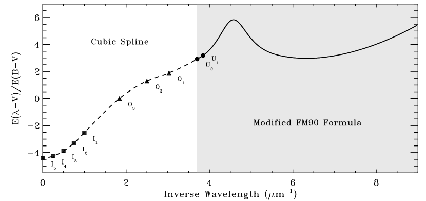
Figure 3: A parametrized representation of normalized UV-through-IR extinction (solid and dashed curve). The curve consists of two parts: 1) $\lambda\leq 2700$ Å (shaded region), where we adopt a modified version of the 3-component parametrization scheme of Paper III; and 2) $\lambda>2700$ Å, where we adopt a cubic spline interpolation through sets of IR ($I_{n}$), optical ($O_{n}$), and UV ($U_{n}$) “anchor points.” The values of the anchor points and the seven parameters describing the UV portion of the curve are determined by fitting the observed SED of a reddened star, as described in §3. The particular curve shown in this figure corresponds to that derived for the star HD147933.

A parametrized representation of the extinction curve, covering the whole UV-through-IR spectral range, is the heart of the current analysis. As in Paper IV, we construct this curve in two parts, joined together at 2700 Å. An example of this formulation, for one particular set of parameters, is illustrated in Figure 3. In the UV, ($\lambda\leq 2700$ Å; the shaded region in the figure), we use a modified form of the UV parametrization scheme of Fitzpatrick & Massa (1990; hereafter Paper III), as shown by the thick solid curve. At longer wavelengths, we use a cubic spline interpolation through a set of UV, optical, and IR “anchor points” (the $U_{n}$, $O_{n}$, and $I_{n}$ in the figure), as shown by the thick dashed curve.

The modified Paper III extinction curve is defined by

$$k(\lambda-V)=\left\{\begin{array}[]{ll}c_{1}+c_{2}x+c_{3}D(x,x_{0},\gamma)&x\leq c_{5}\\ c_{1}+c_{2}x+c_{3}D(x,x_{0},\gamma)+c_{4}(x-c_{5})^{2}&x>c_{5}\;\;,\end{array}\right.$$ (4)

where $x\equiv\lambda^{-1}$, in units of inverse microns ($\mu{\rm m}^{-1}$). There are seven free parameters in the formula which correspond to three features in the curve: (1) a linear component underlying the entire UV wavelength range, defined by $c_{1}$ and $c_{2}$; (2) a Lorentzian-like 2175 Å bump, defined by $c_{3}$, $x_{0}$, and $\gamma$ and expressed as

$$D(x,x_{0},\gamma)=\frac{x^{2}}{(x^{2}-x_{0}^{2})^{2}+x^{2}\gamma^{2}}\;\;;$$ (5)

and (3) a far-UV curvature component (i.e., the departure in the far-UV from the extrapolated bump-plus-linear components), defined by $c_{4}$ and $c_{5}$. All seven free parameters can be determined by the least squares minimization algorithm.

The modification made here to the Paper III formula is in the far-UV curvature term. In Paper III, the value of $c_{5}$ was fixed at 5.9 $\mu{\rm m}^{-1}$ and $c_{4}$ was the scale factor applied to a pre-defined cubic polynomial. In working with the current dataset, we found that the formulation in Equation (4) significantly improved the fits to many stars, particularly those with weak far-UV curvature, and degraded the fits in almost no cases. In the modified form, the curvature is functionally simpler — containing a single quadratic term — although we have added another free parameter to the extinction curve representation. Because the primary goal of the Paper III formula was (and still is) to provide an analytical expression which reproduces as closely as possible observed extinction curves, the cost of an additional free parameter was deemed worthwhile.

Using the UV fit parameters above, additional quantities can be defined which help describe the UV curve properties. Particularly useful ones include 1) $\Delta 1250\equiv c_{4}(8.0-c_{5})^{2}$, which is the value of the FUV curvature term at 1250 Å and provides a measure of the strength of the FUV curvature; 2) $A_{bump}\equiv\pi\;c_{3}/(2\gamma)$, which is the area of the 2175 Å bump; and 3) $E_{bump}\equiv c_{3}/\gamma^{2}$, which is the maximum height of the 2175 Å bump above the background linear extinction.

The cubic spline interpolation which produces the optical-through-IR region of our parametrized extinction curve is produced using the IDL procedure SPLINE. The nine anchor points shown in Figure 3 are specified by five free parameters. The UV points, $U_{1}$ and $U_{2}$, are simply the values at 2600 Å and 2700 Å resulting from the modified Paper III formula and require no new free parameters. They assure that the two separate pieces of the extinction curve will join smoothly, although not formally continuously. The three optical points, $O_{1}$, $O_{2}$, and $O_{3}$ (at 3300 Å, 4000 Å, and 5530 Å, respectively) are each treated as free parameters and are adjusted in the fitting procedure to assure the normalization of the final extinction curve. The IR points, $I_{1}$, $I_{2}$, $I_{3}$, $I_{4}$, and $I_{5}$ (at 0.0, 0.25, 0.50, 0.75, and 1.0 $\mu{\rm m}^{-1}$, respectively) are functions of two free parameters, $k_{IR}$ and $R(V)$ as follows:

$$I_{n}\equiv k(\lambda-V)=k_{IR}\lambda_{n}^{-1.84}-R(V)\;\;.$$ (6)

This assures that the IR portion of our curve follows the the power-law form usually attributed to IR extinction, with a value for its exponent from Martin & Whittet (1990). As noted in Paper IV, the value of the power law exponent could potentially be determined from an analysis like ours. However, we have found that an IR dataset consisting only of JHK magnitudes, as in our survey, is insufficient to specify three IR parameters.

Note that we adopt the cubic spline formulation for the optical/IR extinction curve simply because we do not have an acceptable analytical expression for the curve shape over this range. The spline approach is very flexible in that the number of anchor points can be modified depending on the datasets available. In the current application, we use only three optical anchor points because we have only three optical data points ($V$, $B-V$, and $U-B$). This approach will bear its best fruit when it can be applied to spectrophotometric data in the near-IR through near-UV region. Then, a large number of anchor points can be used to precisely measure the heretofore poorly-determined shape of extinction in this region, without bias towards a particular analytical expression.

In summary, the analysis performed here — modeling the SEDs of 328 reddened stars via Equation (1) — involves determining the best-fit values for as many as 18 free parameters per star, via a non-linear least squares analysis. These include up to 4 parameters to define the theoretical stellar atmosphere model ($T_{\rm eff}$, $\log g$, [m/H], $v_{turb}$), up to 12 parameters to describe the extinction curve shape ($O_{1}$, $O_{2}$, $O_{3}$, $R(V)$, $k_{IR}$, $c_{1}$ through $c_{5}$, $x_{0}$, $\gamma$), the angular radius $\theta_{R}$, and $E(B\!-\!V)$. We weight the UV, optical, and IR datasets equally in the fitting procedure.

3.2 Error Analysis

One of the main benefits of the extinction-without-standards technique is the error analysis, which provides a well-quantified estimate of the uncertainties in the best-fit model parameters and allows possible correlations between parameter errors to be explored. This latter benefit is important for assessing the reality of apparent correlations between parameters. The uncertainties in the best-fit parameters derived for our survey stars were determined by running 100 Monte Carlo simulations for each star. In each simulation, the fitting procedure was applied to an input SED consisting of the final best-fit model convolved with a random realization of the observational errors expected to affect the actual data. The adopted 1-$\sigma$ uncertainties for each parameter, which will be presented in §4, were taken as the standard deviations of the values produced by the 100 simulations.

Our observational error model for the IUE data consists of random photometric uncertainties and camera zero-point errors as described by Fitzpatrick & Massa (2005b). The assumed observational errors in the Johnson $B-V$ and $U-B$ indices were as given in Table 7 of that paper. The $V$ magnitudes were assumed to have a 1-$\sigma$ uncertainty of 0.015 mag. The uncertainties in the 2MASS $JHK$ data were as obtained from the 2MASS archive. Johnson $JHK$ magnitudes were assumed to have uncertainties of $\pm$0.03 mag. Random realizations of each of these observational errors, which were added to the best-fit model SED for each Monte Carlo simulation, were determined using the IDL procedure RANDOMN, which produces a normally distributed random variable.

In cases where assumptions were made about the values of specific fit parameters, we incorporated uncertainties in the assumptions in the error analysis. In particular: (1) for the O-type stars, the adopted spectral type-dependent temperatures were taken to have 1-$\sigma$ uncertainties of $\sim$1000 K; (2) for cluster stars, the adopted distances (used to constrain the surface gravities) were assumed to have 1-$\sigma$ uncertainties of $\pm$20%; and 3) for the field stars whose values of $\log g$ were taken to be the sample mean of 3.9, this mean was assumed to have a 1-$\sigma$ uncertainty of $\pm$0.2. The values of $T_{\rm eff}$, distance, and $\log g$ used in the the Monte Carlo calculations for the relevant stars were varied randomly in the simulations (using RANDOMN) in accord with these uncertainties.

This study certainly does not constitute the first attempt to quantify the uncertainties in interstellar extinction curves. Most pair method studies (see, for example, Cardelli, Sembach, & Mathis 1992) have incorporated some form of error analysis, often based on the methodologies presented by Massa, Savage, & Fitzpatrick (1983) and Massa & Fitzpatrick (1986). However, as long as we restrict our sample to stars which are well represented by the model atmospheres we employ, the advantages of the current technique are great. Because the stellar parameters (temperature, surface gravity, and abundance) are given by continuous mathematical variables (instead of a non-uniformly sampled, discrete sets of standard stars), we are able to perform a well-defined Monte Carlo analysis. The results of this analysis explicitly quantify the uncertainties in all of the input data and assumptions and, thus, the final error bars affecting the derived curves. Moreover, since many realizations of the individual curves are produced, the full shape of the “error ellipses” (which describe correlations between the errors) are determined for each specific set of input parameters. Additional discussion of the extinction-without-standards error analysis can be found in Paper IV of this series, along with a demonstration of the quantitative accuracy of the results.

4 AN ATLAS OF GALACTIC EXTINCTION CURVES

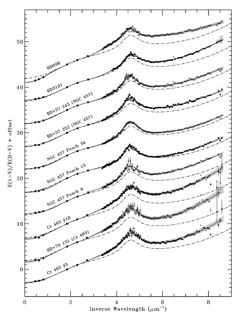
Figure 4: Normalized extinction curves for 328 Galactic stars derived using the extinction-without-standards approach. The symbols show the normalized ratios of the model atmosphere fluxes to 1) the IUE spectrophotometry in the UV ($\lambda^{-1}>3.3\;\mbox{$\mu{\rm m}^{-1}$}$), 2) Johnson UBV photometry in the optical, and 3) Johnson or 2MASS JHK photometry in the near-IR ($\lambda^{-1}<1\;\mbox{$\mu{\rm m}^{-1}$}$). Individual 1-$\sigma$ error bars are shown for the data points, but are typically only visible in the region of the 2175 Å bump and in the far-UV, where the signal level of the IUE data is lowest. Small crosses indicate IUE data points excluded from the fit, for the reasons discussed in Paper IV. IUE data points in the region $1215\leq\lambda\leq 1235$ Å are excluded due to contamination from scattered solar Ly$\alpha$ photons. The solid curves are the parametrized fits to the data as determined by the SED-fitting procedure discussed in §3, and the shaded regions show the 1-$\sigma$ uncertainty in the curves, based on Monte Carlo simulations. For comparison, the dash-dot curves show an estimate of the average Galactic extinction curve from F99 (corresponding to $R(V)=3.1$). Only the first panel of the figure is shown in the print edition of the Journal. The entire figure consists of 33 panels and is available in the electronic edition.

The results of the extinction-without-standards analysis of 328 Galactic stars are presented in Table 3, Table 4, and Figure 4. The 18 free parameters determined by the fitting procedure are divided between Tables 3 and 4, with the latter containing the 12 parameters which define the shape of the normalized interstellar extinction curves $k(\lambda-V)\equiv E(\lambda-V)/E(B-V)$. For both tables, only the first 10 entries are shown here. The full versions of the tables can be viewed in the electronic edition of the Journal. The uncertainties listed in the tables are the 1-$\sigma$ errors derived from the Monte Carlo analysis described in §3.2.

Figure 4 shows the normalized extinction curves for the survey sample. The figure consists of 33 panels, each (except the last) containing 10 extinction curves arbitrarily shifted vertically for clarity. Only the first panel is shown here. The full figure is given in the electronic version of this paper. The solid curves in the figure show the parametrized UV-through-IR curves whose shapes were determined by the fitting procedure described in §3 (the parameters describing the curves are in Table 4). An estimate of the shape of the average Galactic extinction curve (corresponding to $R(V)=3.1$; from Fitzpatrick 1999) is shown for reference by the dash-dot curves. The 1-$\sigma$ uncertainties of the survey extinction curves are indicated in Figure 4 by the grey shaded regions, which are based on the Monte Carlo error simulations. Their thicknesses indicate the standard deviations of the ensemble of simulations at each wavelength. The actual normalized ratios between the observed stellar SEDs and the atmosphere models are shown by the symbols. Large filled circles indicate JHK data in the IR region ($\lambda^{-1}<1\;\mbox{$\mu{\rm m}^{-1}$}$) and UBV data in the optical region ($1.5<\lambda^{-1}<3.0\;\mbox{$\mu{\rm m}^{-1}$}$). In the UV region (($\lambda^{-1}>3.3\;\mbox{$\mu{\rm m}^{-1}$}$), the small symbols with 1-$\sigma$ error bars show the ratios between the IUE data and the models.

A close examination of the curves in Figure 4 shows that the parametrized curves are extremely good representations of the observed extinction ratios and thus serve as useful proxies for the actual curves themselves. This is particularly apparent in the UV, where the spectrophotometric data show the flexibility of the parametrization scheme. For those wishing to use these curves in extinction studies, we have prepared a tar file containing the parametrized curves for all 328 stars, sampled at 0.087 $\mu{\rm m}^{-1}$ intervals, and their accompanying fit parameters. Directions for retrieving the file are given in the Appendix.

In using or interpreting these curves it is important to recognize that their shapes in the regions between the IR and optical and between the UV and optical are interpolations only and not strongly constrained by data. Additional observations, particularly fully-calibrated spectrophotometric data, would be very useful to constrain the shape of the extinction curves in these regions — and in the optical where only broadband UBV measurements are currently employed. It is certainly counter-intuitive that the spectral regions where the detailed shapes of the extinction curves are most poorly-determined are ground-accessible, while the UV data are so well-measured.

5 Properties of the Sample Stars

Although the main goal of this paper is to explore Galactic extinction, it is nevertheless reasonable to consider briefly the stellar properties revealed by our analysis since they directly affect the extinction results. As discussed above, our reliance on broadband photometry for the current work results in stellar parameters that are not as accurate as those presented in Paper IV, due to the lack of a good surface gravity discriminator. Nevertheless, more than 50% of the sample stars reside in open clusters and associations and, for these stars, the accuracy will be increased, due the use of ancillary information.

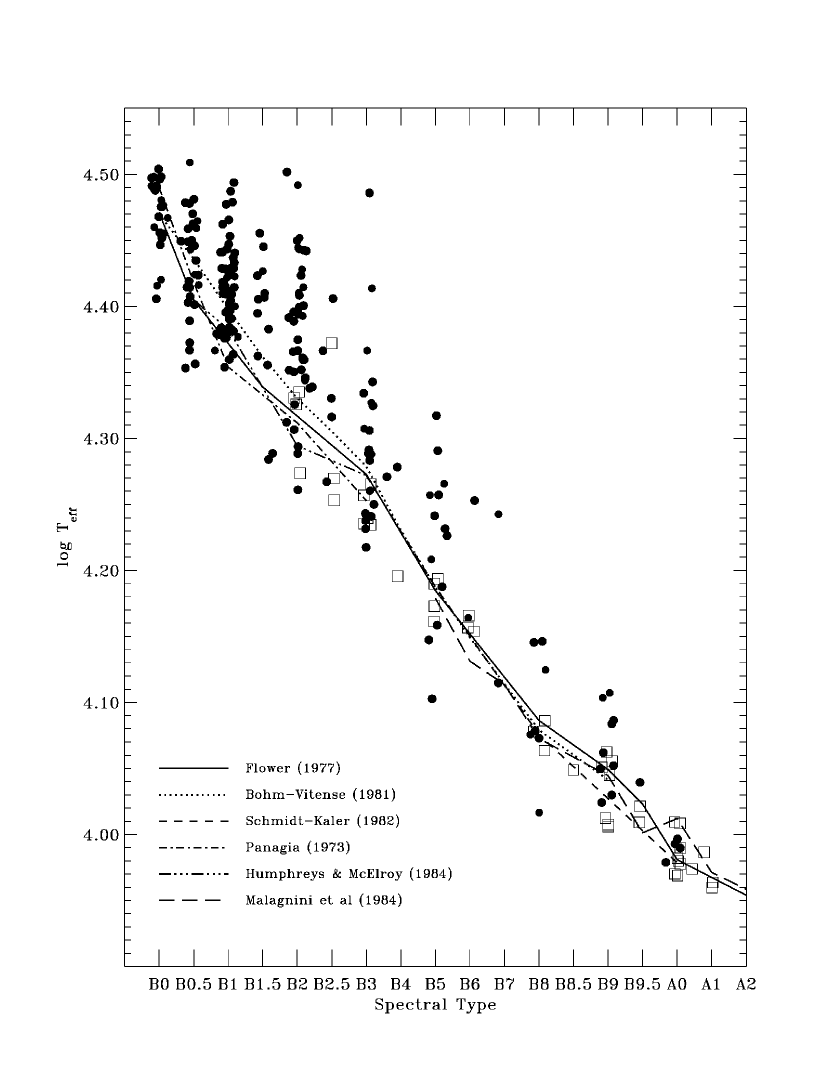
Figure 5: $\log T_{eff}$ as a function of spectral type for the survey stars of type B0 or later. Luminosity class V or IV stars are shown by filled circles; higher luminosity classes by open circles. For comparison, data for the 44 unreddened stars from the photometric calibration study of Fitzpatrick & Massa (2005b) are shown by the open squares. The various dotted, dashed, and solid lines show a number of published spectral type vs. $T_{eff}$ calibrations, as indicated in the figure. Small random horizontal offsets have been added to the data points to increase their visibility.

Of the four stellar properties determined in the analysis ($T_{\rm eff}$, $\log g$, [m/H], $v_{turb}$), the most significant to our extinction program is $T_{\rm eff}$ because it has the most impact on the shapes of the model atmosphere SEDs used to derive the extinction curves. Figure 5 shows a plot of the derived $T_{\rm eff}$ values against spectral type for the spectral class B0 and later stars (filled and open circles). For comparison, we show several spectral type vs. $T_{\rm eff}$ calibrations from the literature (solid and dashed lines) and data from our photometric calibration study (Fitzpatrick & Massa 2005b, open squares) in which we modeled the SEDs of 45 unreddened B-type stars. While the survey star data are generally consistent with the comparison data in the figure, considerable scatter is present at some spectral classes — most particularly at types B2 and B3 — and there is a general departure between our results and the $T_{\rm eff}$ calibrations in the neighborhood of types B1 and B2, in the sense that our results indicate hotter temperatures than the calibrations.

We examined the IUE spectra of a number of the survey stars — those whose temperatures are most discrepant with their claimed spectral types — and compared them with spectral classification standards to see if somehow our fitting procedure was arriving at grossly incorrect temperatures. An example of such a comparison is shown in Figure 6. We plot a portion of the IUE spectra of the survey stars HD228969 and BD+45 973, the two hottest stars in the “B2” and “B3” spectral bins, respectively, along with several spectral standards with expected temperatures in the neighborhood of 30000 K. The close match between the survey stars and the hot standards is evident and it is clear that the cool spectral types found in the literature for these stars are unreliable. This is the general conclusion from all such comparisons we have performed. The temperatures found from the fitting procedure are consistent with those expected from a close examination of the UV spectral features of the stars. We conclude that the outliers in Figure 5 result from poor optical spectral types. This is not surprising, since the available types are from a large number of sources and based on a wide variety of observational material of very non-uniform quality.

The general discrepancy between our results and the calibrations in the B1-B2 region is a different matter. We derive considerably hotter effective temperatures for the B1 (25000 – 26000 K) and B2 (23000 – 24000 K) stars than expected from previous calibrations. However, inspection of the UV features in the ATLAS9 models make it difficult to believe that typical B1 and B2 stars are as cool as the spectral type – $T_{\rm eff}$ calibrations suggest. We must bear in mind, however, that our sample is strongly biased toward cluster stars, which may be considerably younger and more compact than the “field” B stars used in the calibrations. Furthermore, the current B star calibrations are all over 20 years old, and it is quite possible that they are in need of revision.

Another way to look at the $T_{\rm eff}$ values is shown in Figure 7 where we plot $T_{\rm eff}$ as a function of the Strömgren reddening-free index $[c]\equiv c_{1}-0.20(b-y)$, which is a measure of the strength of the Balmer jump. Strömgren photometry is not used in this program but is available for 162 of our stars. The symbols in Figure 7 are the same as in Figure 5, with the addition of the open circles which denote O stars. The figure demonstrates the essentially exact overlap between the current results and those for the unreddened, mid-to-late B stars from Fitzpatrick & Massa (2005b) as well as the smooth transition from the early B stars into the O stars. There is no indication of any systematic effects present in the results for the early B stars. On the contrary, the spectral type vs. $T_{\rm eff}$ relations, transformed into the $T_{\rm eff}$ vs. $[c]$ plane as described in the figure legend, show a number of abrupt and physically unrealistic changes in slope suggestive of inadequacies in the calibrations.

We conclude that our derived effective temperatures are reasonable. In most cases where a temperature strongly disagrees with a published MK type, it agrees quite well with the UV type determined by Valencic, Clayton, & Gordon (2004), indicating that the MK type is of poor quality or else influenced by something else (e.g., the presence of a cooler companion which is invisible in the UV). We also suspect that the spectral type – $T_{\rm eff}$ calibration for the B1 and B2 stars may need to be revised. Finally, we are gratified by the overall consistency between the current results and those of Paper IV and Fitzpatrick & Massa (2005b), where the stellar parameters were more strongly constrained, and with the smooth relation between $T_{\rm eff}$ and [c], which suggests that no strong systematic effects are present.

6 Properties of Galactic Interstellar Extinction

6.1 General Properties

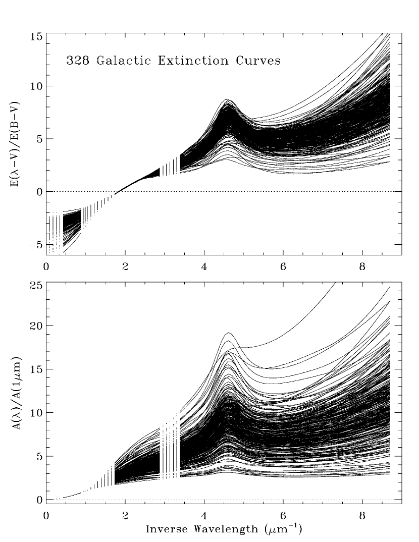
Figure 8: Analytical representations of 328 Galactic UV-through-IR extinction curves plotted in their native normalization $E(\lambda-V)/E(B-V)$ (top panel) and transformed into an IR-normalized form $A(\lambda)/A(1\/\mu{\rm m})$ (bottom panel). The curves, in their standard form, can be reproduced from the parameters given in Table 4. The convergence of the curves in the optical region (top panel) and the IR region (bottom panel) results from their normalizations. The value of $R(V)\equiv A(V)/E(B-V)$ for each curve is the negative of its intercept at $\lambda^{-1}=0\;\mbox{$\mu{\rm m}^{-1}$}$ in the $E(\lambda-V)/E(B-V)$ panel.

Although the individual extinction curves for all of the survey stars are displayed in the 33 panels of Figure 4, it is nonetheless difficult — from that figure — to visualize the range of extinction properties present in the sample. To provide such a view, we plot the analytical fits for the full set of 328 survey curves in Figure 8. (These curves can be reproduced from the parameters listed in Table 4. The curves have been plotted using small dots in those spectral ranges where they are interpolated or extrapolated. The solid portions correspond to the regions constrained by near-IR JHK photometry, optical UBV photometry, and UV IUE spectrophotometry. The top panel, in which the curves are plotted in their native form, $E(\lambda-V)/E(B-V)$, shows the wide range of variation observed in Galactic extinction curves, although a clear core of much more restricted variation is evident in the distribution. The convergence of the curves in the range $1.8<\lambda^{-1}<2.5~{}\mbox{$\mu{\rm m}^{-1}$}$ is a product of the normalization and obscures our view of variations in the optical region. The bottom panel of Figure 8 presents the same curves, but normalized to the total extinction at 1 $\mu{\rm m}^{-1}$. The exact overlap of the curves at $\lambda^{-1}<1~{}\mbox{$\mu{\rm m}^{-1}$}$ arises because we have adopted a power law form with a fixed exponent of $-1.84$ for all curves in this spectral region (see Eq. [6]). It is unlikely that the exponent is actually so constant — Larson & Whittet (2005) have found evidence for a more negative value in a sample of high-latitude clouds — however, as noted earlier in §3, our near-IR dataset consisting of only JHK measurements is insufficient for independently evaluating the exponent. This IR normalization reveals that the extinction in the optical spectral region can range from very-nearly grey to very strongly wavelength-dependent.

One of the goals of many Galactic extinction studies is to derive an estimate of the typical or average wavelength-dependence of interstellar extinction. Such a mean curve is often used as the standard of normalcy against which particular sightlines are judged, or for comparison with results for external galaxies, or for “dereddening” the SEDs of objects for which there is no specific extinction knowledge. While constructing an average curve is a straightforward process, the degree to which the result represents “normal” or even “typical” extinction is problematic. We will take up the issue of an average Galactic curve later in §7. Here we present an average curve for our sample, to help characterize the general extinction properties of our survey sightlines.

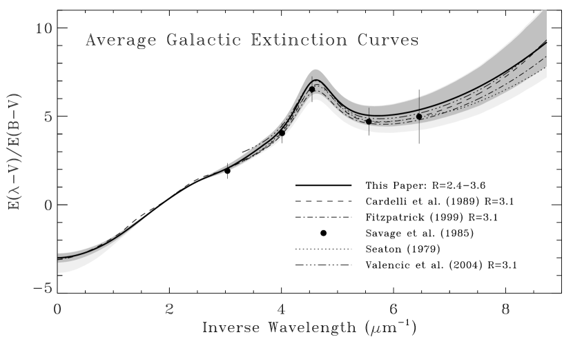
Figure 9: An average UV-through-IR extinction curve for our sample compared with other mean extinction curves. The thick solid curve is the mean for the 243 stars in our sample with $2.4<R(V)<3.6$, i.e., for those sightlines with $R(V)$ values indicative of the diffuse ISM. The dark gray shaded region shows the sample variance about the mean curve at all wavelengths. The light grey shaded area shows the larger variance that results when we include all 298 sightlines with measured $R(V)$ values. The mean curve can be reconstructed from the extinction parameters listed in Table 5. The dashed and dotted curves show estimates of mean UV Galactic curves from the sources indicated in the figure. The large filled circles are means from the ANS satellite extinction catalog of Savage et al. (1985) for 800 stars with $\mbox{$E(B\!-\!V)$}\geq 0.20$ mag. These measurements result from filter photometry centered at wavelengths of 3000, 2500, 2200, 1800, and 1550 Å. Error bars on the ANS data show the sample variances and include the effects of spectral mismatch.

The bottom panel in Figure 2 shows a clear peak in the distribution of $R(V)$ values of our sample. A Gaussian fit to the region of this peak, shown as the smooth curve in the figure, has a centroid at $R(V)=2.99$ and a width given by $\sigma=0.27$. The peak is within the range of values considered as average for the diffuse ISM (see, e.g., Savage & Mathis 1979). Thus, as noted in §2, our sample is dominated by sightlines whose $R(V)$ values are consistent with the diffuse phase of the ISM (although composite sightlines are undoubtedly present). We have constructed an average curve to represent the properties of these diffuse sightlines by taking the simple mean extinction value at each wavelength using all the curves with $2.4<R(V)<3.6$ (i.e., the  2-$\sigma$ range of the Gaussian fit in Figure 2; 243 sightlines in total). This mean extinction curve is shown in Figure 9 by the thick solid curve. The dark grey shaded region shows the variance of the 243-curve sample. The set of 12 parameters describing this curve are listed in Table 5. Since so many of our sightlines are included in the mean, removing the restriction on $R(V)$ has little effect. If we had included all 298 sightlines for which $R(V)$ has been derived, then the mean curve would differ from that shown only by being several tenths lower in the UV region. The variance of the full sample is larger, and this is shown by the lightly shaded region. For comparison, several other estimates of average Galactic curves are shown in Figure 9. The curves from Cardelli et al. (1989), Fitzpatrick (1999), Seaton (1979), and Valencic et al. (2004) are all intended to represent the diffuse ISM mean. The results from Savage et al. (1985) are mean values for the 800 sightlines in that study with $E(B-V)\geq 0.20$ mag (matching our survey cutoff). No restriction on $R(V)$ was imposed. The error bars for the Savage et al. (1985) data are sample variances; they are generally similar to the variances of our full sample (lightly shaded region). The much larger value for the 1500 Å point is likely due to spectral mismatch in the potentially strong C IV stellar wind lines.

The differences among the various mean curves in Figure 9 are instructive. The great intrinsic variety of Galactic extinction curves as seen, for example, in Figure 8 shows that any mean curve is subject to the biases in the sample from which it was produced. It is probably impossible to construct a sample of sightlines whose properties could be claimed to provide a fair representation of all the types of conditions found in the ISM. Thus, there is likely no unique or best estimate of mean Galactic extinction. Any of the mean curves in Figure 9 would serve as reasonable representations of Galactic extinction. In any situation where an average curve is adopted, however, it is important to recognize the intrinsic variance of the underlying sample and incorporate the uncertainties of the average curve in any error analysis. Because it is derived from such a large sample and is largely free of contributions from spectral mismatch, the sample variance for our diffuse curves (shown in Figure 9 by dark shaded region) would provide a reasonable estimate of the uncertainty in any version of a mean Galactic diffuse ISM curve. We have included our diffuse ISM mean curve from Figure 9 — and its accompanying uncertainty — in the tar file discussed in §4 (see the Appendix).

We can also use our large sample to investigate the “smoothness” of UV extinction. In Figure 10, we plot the simple mean of the actual extinction ratios for our survey sample in the spectral region covered by the IUE data (upper curve, open circles). Overplotted is a parameterized fit to these data, using the extinction formulation given in §3 (solid curve). This figure illustrates two points; namely, 1) the lack of small-scale structure in UV extinction and 2) the degree to which the modified Paper III UV parametrization scheme reproduces the shape of UV extinction. A detailed discussion of the former point, and an indication of the kinds of features that might be expected in the UV, can be found in Clayton et al. (2003). In short, polycyclic aromatic hydrocarbon (PAH) molecules, which have been suggested as the source of mid-IR emission features, might produce noticeable absorption in the UV, and possibly even contribute to the 2175 Å bump absorption. Earlier studies have always failed to find structure in UV extinction curves and Clayton et al. were able to place very stringent 3-$\sigma$ upper limits of $\sim 0.02A_{V}$ on any possible 20 Å-wide features in the extinction curves towards two heavily reddened B stars. The data at the bottom of Figure 10 show the differences between the mean extinction curve and the best-fit model. A small number of points do rise above (or below) the general noise level of the residuals, but these points — which are labeled in the figure — are due to interstellar gas absorption lines (which are sometimes strong in the observations and always non-existent in the model atmosphere SEDs), mismatch between the C IV $\lambda$1550 stellar wind lines in the O stars and the static model SEDs, or known inadequacies in the ATLAS9 opacity distribution functions (labeled “b” in the figure; see Paper IV). Excluding these points, the standard deviation of the mean curve around the best-fit is 0.06$E(B\!-\!V)$ mag, corresponding to $\sim 0.02A_{V}$ mag, for the 10 Å-wide spectral bins. This is not quite so restrictive as the result of Clayton et al., but once again affirms the smoothness of UV extinction.

6.2 Spatial Trends

Studying spatial trends in extinction can serve two purposes. First, identifying strong regional variations can allow a better estimate of the shape of the extinction curve affecting a particular sightline permitting, for example, a more accurate determination of the intrinsic SED shape of an exotic object. This has been the motivation for a number of studies, such as by Massa & Savage (1981) and Torres (1987) who used extinction curves derived for B stars in open clusters (NGC 2244 and NGC 6530, respectively) to determine the SEDs of cluster O stars. The second purpose is to gain insight into the nature of dust grains and the processes which modify them by observing how extinction curves respond to various environmental properties, such as density or radiation field.

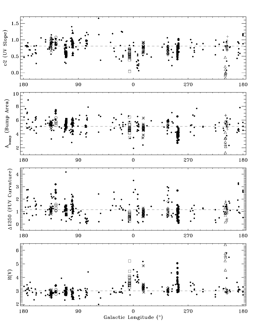
Figure 11: Spatial trends in extinction properties. The values of four parameters which describe the shapes of interstellar extinction curves are plotted against Galactic longitude for each of our survey sightlines. Small filled circles show field sightlines. Other symbols denote sightlines to clusters or associations for which five or more members are included in our survey. From left to right, the clusters are: h & $\chi$ Per (x’s); NGC 457 (open circles); Cr 463 (filled diamonds); Cep OB3 (filled squares); Trumpler 37 (filled triangles); NGC 6530 (open squares); NGC 6231 (*’s); NGC 4755 (open diamonds); Carina clusters (large filled circles, includes Trumpler 14 and 16, Cr 228, and NGC 3293); NGC 1977 (open triangles); and NGC2244 (+’s). The dashed lines show the parameter values corresponding to the diffuse mean ISM curve from Figure 9.

In Figure 11 we show a sweeping view of the regional trends in our data by plotting several extinction curves properties against Galactic longitude for each of our survey sightlines. Sightlines towards stars in the clusters or associations highlighted in Figure 1 are indicated by the larger symbols in Figure 11 (the key is in figure caption) and the rest of the sample by the small filled circles. The dashed lines in the figure panels show the parameter values that correspond to the diffuse mean curve in Figure 9.

A number of regions stand out in Figure 11. For example, NGC 1977 near $l=210\arcdeg$ (open triangles; includes the Orion Trapezium region) is well-known for its high $R(V)$ sightlines. Figure 11 shows that this region is also notable for its flat UV extinction curves (i.e., small $c_{2}$) and weak bumps (i.e., small $A_{bump}$). Interestingly, the far-UV curvature for this region appears typical. An early discussion of UV extinction curves towards NGC 1977 can be found in Panek (1983). The relationship between $R(V)$ and other curve properties will be the subject of §6.4 below.

The Carina direction (large filled circles), particularly towards Tr 14 and Tr 16, also shows elevated $R(V)$ values. This is another weak-bumped direction which also shows lower than average FUV curvature. Optical and IR extinction studies have been performed for Carina sightlines (e.g., Tapia et al. 1988 and references within), but we are not aware of correspondingly detailed UV extinction studies.

Large $R(V)$ values are also seen along a number of sightlines in the general direction of the Galactic center. This includes sightlines to the cluster NGC 6530 (open squares) and towards the $\rho$ Oph dark cloud (small filled circles near $l\simeq 253\arcdeg$. These sightlines also feature low UV extinction and, in the case of NGC 6530, weaker than average 2175 Å bumps. Large $R(V)$ are well known in the Ophiuchus region (Chini & Krugel 1983) and the UV extinction has been examined by Wu, Gilra, & van Duinen (1980). UV extinction towards NGC 6530 was studied by Torres (1987).

Finally we note a broad region from $l\simeq 50\arcdeg$ to $l\simeq 150\arcdeg$ where the $R(V)$ values are systematically slightly below the mean value. No trends are obvious in the UV parameters. These sightlines are in the direction of the Perseus spiral arm (e.g., Georgelin & Georgelin 1976) and sample dust in the interarm region and, possibly, the Perseus Arm itself — for those stars more distant than $\sim$2 kpc, such as in h & $\chi$ Per (x’s in Figure 11). Extinction towards individual regions in this zone have been studied (e.g., Tr 37 by Clayton & Fitzpatrick 1987, Cep OB3 by Massa & Savage 1984, h & $\chi$ Per by Morgan, McLachlan, & Nandy 1982, and Cr 457 by Rosenzweig & Morrison 1986), but we are not aware of any comprehensive investigation of the general region.

Morgan et al. (1982) found a dependence of UV extinction on Galactic latitude, $b$, for sightlines to stars in h & $\chi$ Per, in the sense that the extinction at 1550 Å increases with increasingly negative values of $b$. Our data suggest a similar effect for the UV linear slope $c_{2}$ (which is closely related to the extinction level at 1550 Å), but not for any other extinction parameter, including $R(V)$. We have examined our dataset for general trends with Galactic latitude, or with distance above and below the plane, and have found none. This is not surprising, however, since our sample is dominated by low-latitude sightlines and we have little leverage for a latitude-dependence study. Our lower cutoff of 0.20 mag in $E(B\!-\!V)$ eliminated most high-latitude sightlines from consideration. Previous studies have shown that it is difficult to uncover latitude dependences in extinction (e.g., Kiszkurno-Koziej & Lequeux 1987). Local trends might be uncovered by examining small zones in Galactic longitude (such as in the study by Morgan et al.), although such detailed investigations are beyond the scope of this paper. Likewise, studies of extinction variations over small spatial scales, such as among sightlines to cluster members are beyond our scope, but might well provide important information linking grain populations with other ISM diagnostics.

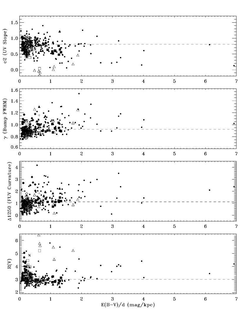
Figure 12: Density trends in extinction properties. The values of four parameters which describe the shapes of interstellar extinction curves are plotted against $E(B\!-\!V)$$/d$ for our survey sightlines. Small filled circles are field sightlines. Other symbols (same as in Figure 11) denote sightlines to clusters or associations containing five or more survey stars. The dashed lines show the parameter values corresponding to the diffuse mean ISM curve in Figure 9. 9.

The quantity $\mbox{$E(B\!-\!V)$}/d$, which can be computed from the data in Tables An Analysis of the Shapes of Interstellar Extinction Curves. V. The IR-Through-UV Curve Morphology and 3, provides a crude measure of one important physical property of the ISM, namely, dust density. While the shortcomings of this measure as a direct proxy for density are clear — for example, a high density dust cloud along a long, otherwise vacant sightline will yield a misleadingly low value of $\mbox{$E(B\!-\!V)$}/d$ — it is nevertheless useful as a first-look and as a guide for future studies. Figure 12 shows plots of four extinction curve parameters against $\mbox{$E(B\!-\!V)$}/d$. The symbols are the same as for Figure 11. The three UV parameters all show evidence for a weak trend with density, in the sense of flatter slopes, broader bumps, and increasing FUV curvature with increasing density. Hints of these three effects were seen in the first two papers in this series (Fitzpatrick & Massa 1986, 1988; hereafter Papers I and II). We see no evidence for a trend with bump strength $A_{bump}$ (not shown in Figure 12) and the dependence of $R(V)$ on $\mbox{$E(B\!-\!V)$}/d$ is complex and difficult to characterize, although the highest density sightlines all have larger-than-average values of $R(V)$. While not conclusive, the results in Figure 12 certainly suggest that comparisons of our survey data with detailed measures of ISM physical conditions could yield interesting results. We note that Rachford et al. (2002) have found positive trends of bump width and far-UV curvature with the fraction of hydrogen atoms in the form H₂. This is consistent with the results in Figure 12 in the sense that one would expect higher H₂ fractions in denser, and therefore better-shielded, regions. Other studies of the density-dependence of extinction have been performed by Massa (1987) and Clayton, Gordon, & Wolff (2000).

6.3 Relationships Among the Fit Parameters

With twelve parameters to describe the UV-through-IR extinction curves of each of the 328 survey stars, there are many possible correlations and relationships to investigate. We have looked at all of these possibilities and, as an interested reader can verify from the data in Table 4, virtually all the parameters are remarkably UNcorrelated with each other! In this section, we consider only the two most striking relationships between extinction parameters: $c_{1}$ vs. $c_{2}$ (the UV linear intercept and slope) and $R(V)$ vs. $k_{IR}$ (the ratio of selective-to-total extinction and the IR scale factor). We also examine the most important non-relationship between parameters: $x_{0}$ vs. $\gamma$ (the centroid and width of the 2175 Å bump). Below, in §6.4, we will consider the possible relationship between IR curve features and UV features.

6.3.1 $c_{1}$ vs. $c_{2}$

In Papers I and II we showed that pair method extinction curves in the region of the 2175 Å extinction bump could be modeled very precisely using a Lorentzian-like “Drude profile” (see Eq. [5]) combined with a linear background extinction (defined by the parameters $c_{1}$ and $c_{2}$ in Eq. [4]). Further, it was shown that the linear parameters for the 45 sightlines in the study appeared to be very well correlated, and could likely be replaced with a single parameter without loss of accuracy. In the pilot study for this paper, F04 showed that this correlation was maintained in a larger sample of 96 curves derived using the extinction-without-standards technique.

Figure 13 shows a plot of the linear parameters $c_{1}$ vs. $c_{2}$ for our survey sample of 328 extinction-without-standards curves. The dotted error bars show the orientation of the 1-$\sigma$ error ellipses of the measurements. These were determined by the distribution of results from the Monte Carlo simulations. The obvious correlation between the errors in $c_{1}$ and $c_{2}$ is not unanticipated (see Figure 4 in Paper II), but the ability to explicitly determine such errors is a major advantage of the extinction-without-standards approach and is critical for evaluating the significance of apparent correlations.

The solid line in Figure 13 corresponds to the linear relation

$$c_{1}=2.09-2.84\;c_{2}\;\;,$$ (7)

which is a weighted fit that minimizes the scatter in the direction perpendicular to the fit. (Because there is uncertainty in both $c_{1}$ and $c_{2}$, a normal least squares fit is not appropriate.) The fact that this relationship is nearly parallel to the long axis of the correlated error bars explains why the relationship between $c_{1}$ and $c_{2}$ remains so clear, even in the presence of observational error.

To determine whether the observed scatter about the mean $c_{1}$ vs $c_{2}$ relationship is caused only by observational error or is at least partially the result of “cosmic” scatter, we must examine the residuals to the best-fit relationship. The distribution of residuals perpendicular to the best-fit line is complex, consisting of a Gaussian core of values with $\sigma\simeq 0.07$ and a more extended distribution of outliers reaching out to values of about $\pm 0.3$. About 86% of the points fall within the 2-$\sigma$ range of the Gaussian core. The RMS value of the expected observational errors perpendicular to the best-fit relation is 0.057. The Gaussian core of the observed residuals is thus only slightly broader than that expected from observational scatter alone. We conclude that $c_{1}$ and $c_{2}$ are indeed intrinsically well-correlated quantities, with a cosmic scatter comparable to our measurements errors. However a significant fraction of the sample ($\sim$10%) show evidence for a wider deviation from the mean relationship. In most instances, Equation (4) could be simplified without loss of accuracy by replacing the two linear parameters $c_{1}$ and $c_{2}$ with a single parameter.

6.3.2 $R(V)$ vs. $k_{IR}$

F04 showed that the two parameters describing the IR portion of the extinction-without-standards curves, $k_{IR}$ and $R(V)$ are apparently well-correlated and that the IR curve might be defined by a single parameter. Figure 14 shows a plot of $k_{IR}$ vs. $R(V)$ for the survey sample, along with the 1-$\sigma$ error bars. The solid curve shows the best-fit weighted linear relationship

$$k_{IR}=-0.83+0.63\;R(V)\;\;,$$ (8)

which minimizes the scatter in the direction perpendicular to the relation. As in the discussion above, we see that the errors are strongly correlated and the near coincidence of the long axis of the error ellipses with the direction of the best-fit relationship would preserve the appearance of a correlation even in the face of significant observational error. The residuals in the direction perpendicular to the best-fit line are distributed in a Gaussian form, with $\sigma=0.11$. The RMS value of the observational errors in this same direction is $\pm 0.12$. Thus the observed distribution of points in Figure 14 is consistent with perfectly correlated quantities and the expected observational error.

The correlation between $R(V)$ and $k_{IR}$ indicates that the shape of near-IR extinction at $\lambda>$ $\sim$1 $\mu{\rm m}$, over a wide range of $R(V)$ values, can be characterized by a single parameter. I.e., the two parameters in Equation (6) are redundant and could be replaced — without loss of accuracy — by a single parameter, e.g., $R(V$), based on Equation (8):

$$\frac{E(\lambda-V)}{E(B-V)}=[-0.83+0.63R(V)]\lambda^{-1.84}-R(V)\;\;.$$ (9)

This is consistent with the results of Martin & Whittet (1990; see their Table 2), who utilized IR data out to the $M$ band near 5 $\mu$m. Our study utilizes only shorter wavelength near-IR bands, but includes many more sightlines and spans a wider range in $R(V)$ values than could be studied by Martin and Whittet. Our parameter $k_{IR}$ is essentially the same as their $e$ parameter, and our results demonstrate the dependence of $e$ on $R(V)$.

The significance of the tight correlation between $R(V)$ and $k_{IR}$ is somewhat difficult to assess. We must keep in mind that, at one level, this relation simply states that the three IR data points given by 2MASS $JHK$ photometry can be summarized by two parameters at the level of the errors in the 2MASS photometry. On the other hand, it also bears on the issue of the underlying shape of infrared extinction and its so-called universality. Our data, which are dominated by diffuse ISM sightlines, are consistent with the notion of a universal shape for IR extinction, as given by Equation (9). However, given our restricted IR wavelength coverage and the typical uncertainties in the 2MASS data, our results are relatively insensitive to departures from universality. For example, the actual IR power law exponent among our sample stars could vary significantly around the mean value of $-1.84$ used here, and we would still find a very strong correlation between $k_{IR}$ and $R(V)$. The issue of the universality of IR extinction is best left to indepth studies which utilize more focussed approaches and more appropriate datasets, such as by Larson & Whittet (2005) and Nishiyama et al. (2006), both of which have found a range in values for the IR exponent.

Values for $R(V)$ are often estimated from the formula $R(V)=1.1E(V-K)/E(B-V)$, which is based on van de Hulst’s theoretical extinction curve No. 15 (e.g., Johnson 1968). In Figure 15 we plot $E(V-K)/E(B-V)$ vs. $R(V)$ for our survey sightlines. The dotted line shows the van de Hulst relation, which agrees well with the data for values of $R(V)$ near 3 — not surprising since it was derived from a theoretical curve with R = 3.05 — but systematically deviates at higher and lower values of $R(V)$. The solid line in the figure shows the best-fit linear relation which minimizes the residuals perpendicular to the fit. It is given by

$$R(V)=-0.26+1.19\;\frac{E(V-K)}{E(B-V)}\;\;.$$ (10)

This relationship was derived only from the sightlines with 2MASS $K$-band measurements (solid circles in Figure 15) but also agrees with those measurements based on Johnson $K$-band photometry (open circles). This exact form of this relation depends slightly on our choice of an IR power law exponent of $-1.84$, and the small scatter is another indicator that our data are consistent with a single functional form for IR extinction. The relationship in Equation (10) can be reproduced by Equation (9) with a wavelength of $\lambda\simeq 2.1\;\mu$m.

6.3.3 $x_{0}$ vs. $\gamma$

Among the many non-correlations between extinction quantities, one of the most significant is that between the position of the peak of the 2175 Å bump (parametrized here by $x_{0}$) and its FWHM (parametrized by $\gamma$). The lack of a relationship between these two quantities, as first reported in Paper I, places strong constraints on the nature of the dust grains which produce the 2175 Å feature (see, e.g., Draine 2003).

Figure 16 shows a plot of $\gamma$ vs. $x_{0}$ for our survey sightlines, along with their 1-$\sigma$ error bars. As in all previous studies, the lack of a correlation is clear.

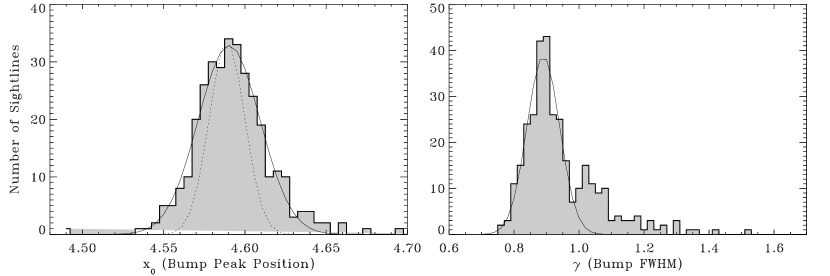
Figure 17: 2175 Å bump statistics. The left panel shows a histogram of the distribution of the 2175 Å bump peak positions for our sample. The smooth curve is a Gaussian fit centered at $x_{0}=4.5903\;\mbox{$\mu{\rm m}^{-1}$}$ (2178.5 Å) with a width of $\sigma=0.0191\;\mbox{$\mu{\rm m}^{-1}$}$ (9.1 Å). The RMS value of the measurement errors in $x_{0}$ is $\pm 0.0058\;\mbox{$\mu{\rm m}^{-1}$}$ ($\pm 2.8\;{\rm\AA}$). The dashed curve shows a Gaussian fit to the distribution of bump positions for 154 stars located in the 13 open clusters with more than 5 stars in the survey. For each cluster, a mean value of $x_{0}$ was computed and the distributions constructed relative to the mean (see §6.3.3). The width of the cluster Gaussian is given by $\sigma=0.011\;\mbox{$\mu{\rm m}^{-1}$}$ (5.2 Å). The right panel shows the distribution of bump FWHM values. The smooth curve is a Gaussian fit to the main peak in the distribution. Its central position corresponds to $\gamma=0.890\;\mbox{$\mu{\rm m}^{-1}$}$ and its width is $\sigma=0.050\;\mbox{$\mu{\rm m}^{-1}$}$. The RMS measurement error in $\gamma$ is $\pm 0.031\;\mbox{$\mu{\rm m}^{-1}$}$.

Figure 17 shows the distribution of bump peak positions (left panel) and widths (right panel) plotted in histogram form (shaded regions). With the exception of a few outliers, the distribution of bump peaks can be fitted well with a Gaussian function, as indicated in Figure 17 by the smooth solid curve. The centroid of the Gaussian is at $x_{0}=4.5903$ $\mu{\rm m}^{-1}$ and its width is given by $\sigma=0.0191$ $\mu{\rm m}^{-1}$. These correspond to a mean bump position of 2178.5 Å with a 1-$\sigma$ range of $\pm 9.1$ Å. The RMS value of the $x_{0}$ measurement errors for the full sample is $\pm 0.0058$ $\mu{\rm m}^{-1}$ (corresponding to $\pm 2.8$ Å).

While these results suggest small but significant variations in bump positions — as reported in Paper I — the Gaussian-like distribution of $x_{0}$ values in Figure 16 led us to consider that perhaps our error analysis might underestimate the uncertainties in $x_{0}$ and that the width of the Gaussian itself might represent the true observational error. We examined this issue by considering the results for sightlines towards stars in open clusters and associations. We have previously used such sightlines to help estimate extinction curve measurement uncertainties (Massa & Fitzpatrick 1986). If it is assumed that the true extinction curve is identical for all cluster sightlines (based on the small spatial separation between the sightlines), then each cluster curve represents an independent measurement of the same curve and the variations from sightline-to-sightline give the net measurement errors. Since it is unlikely that there is no cosmic variability among the sightlines, this procedure provides upper limits on observational errors. We utilized data for the 13 clusters with five or more stars in our survey (NGC 457, Cr 463, NGC 869, NGC 884, NGC 1977, NGC 2244, NGC 3293, Tr 16, NGC 4755, NGC 6231, NGC 6530, Tr 37, and Cep OB3), yielding a total of 154 sightlines. For each cluster we computed the mean value of $x_{0}$ and subtracted it from the individual cluster values. We then examined the ensemble of residuals for the full cluster sample. The shape of the residuals distribution is Gaussian-like, although very slightly skewed towards positive values. A Gaussian fit yields the result shown by the dotted curve in the $x_{0}$ panel of Figure 16 (scaled to match the height of the main distribution), which has a width given by $\sigma=0.011$ $\mu{\rm m}^{-1}$. This is larger than the RMS measurement error for the cluster sample, i.e., $\pm 0.0058$ $\mu{\rm m}^{-1}$, but significantly smaller than the observed width of the full sample. For a number of the clusters, there are obvious curve-to-curve variations present, and the width of the residuals distribution must certainly overestimate the measurement errors. From this more detailed analysis, our conclusion remains that the small variations of $\pm 9.1$ Å seen in the full survey sample, are significantly larger than the expected observational errors and indicate true variations in the position of the bump peak.

The distribution of bump widths (right panel of Figure 17) is decidedly non-Gaussian, with a strong tail in the direction of large values. The main peak of the distribution, however, is Gaussian in appearance and a fit to this region (smooth curve in the figure) yields a centroid of 0.890 $\mu{\rm m}^{-1}$ and a width of $\sigma=0.050$ $\mu{\rm m}^{-1}$. The RMS value of the observational errors is $\pm 0.031$ $\mu{\rm m}^{-1}$, and so the width of this Gaussian, and the width of the whole distribution is clearly larger than can be accounted for by observational errors. Again consistent with earlier results, we find that the bump widths vary significantly from sightline to sightline, but with no correlation with the centroid position. The shape of the $\gamma$ distribution might suggestion two populations of bumps — one characterized by the Gaussian fit and the other characterized by a larger mean centroid ($\sim$1.1 $\mu{\rm m}^{-1}$) and a wider range of values ($\sigma\simeq 0.1$ $\mu{\rm m}^{-1}$), but this is not the only possible interpretation of the results. We examined the bump widths for the cluster sample as above. However, the distribution of cluster residuals is complex, showing the asymmetry of the full sample, and indicating significant variations within the clusters, and we were thus not able to confirm the accuracy of the measurement errors. The range in observed $\gamma$ values is so large, however, that the evidence for cosmic scatter is unambiguous.

6.4 $R(V)$-Dependence

Cardelli, Clayton, & Mathis (1988, 1989) were the first to demonstrate a link between UV and optical/IR extinction by showing that $R(V)$ is related to the level of UV extinction. Essentially, sightlines with large $R(V)$ values tend to have low UV extinction, and vice versa. Cardelli et al. quantified this relationship in the following way:

$$\frac{A(\lambda)}{A(V)}=a(\lambda)+b(\lambda)\;R(V)^{-1}\;\;\;\;;$$ (11)

i.e., the total extinction at wavelength $\lambda$ normalized by the total extinction at $V$ is a linear function of $R(V)^{-1}$. In the time since the original work, the perception of this relationship has evolved to the point where it is often referred to as a “law” and Galactic extinction curves are often stated or assumed to be a 1-parameter family (with $R(V)^{-1}$ as the parameter). Recently, for example, Valencic et al. (2004) found that 93% of a large sample of Galactic extinction curves obey a modified form of this relation. In this section, we will show that the relationship in Equation (11) is partially illusory and that Galactic extinction curves are decidedly not a 1-parameter family in $R(V)^{-1}$.

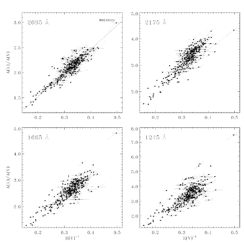
Figure 18: Plots of the normalized extinction values $A(\lambda)/A(V)$ vs. $R(V)^{-1}$ at four different UV wavelengths. $A(\lambda)/A(V)$ is derived from the measured values of $E(\lambda-V)/E(B-V)$ by using Equation (12). 1-$\sigma$ error bars are shown, based on our Monte Carlo simulations. The error bars, which are not orthogonal to each other because the scales of the x- and y-axes are different, show the clear correlation in the uncertainties for $A(\lambda)/A(V)$ and $R(V)^{-1}$. The straight line in the 2695 Å panel is a weighted linear fit to the data, which minimizes the scatter perpendicular to the relation. It is given by $A(2695\;{\rm\AA})/A(V)=0.58+4.73\;R(V)^{-1}$.

The original basis for Equation (11) is data such as shown in Figure 18, where we plot $A(\lambda)/A(V)$ vs. $R(V)^{-1}$ at four different UV wavelengths for our survey sightlines (see Figure 1 in Cardelli et al. 1989). It is clear why a linear function would be chosen to quantify the obvious relationships seen in the figure, and the data give the impression of being reasonably well-correlated. The solid line in the 2695 Å panel shows an example of such a linear relationship. It is a weighted fit which minimizes the residuals in the direction perpendicular to the fit, and is given by $A(2695\;{\rm\AA})/A(V)=0.58+4.73\;R(V)^{-1}$. The appearance of Figure 18 is, however, deceiving. The normalization used in the y-axis is constructed from the measured values of $E(\lambda-V)/E(B-V)$ by the transformation

$$\frac{A(\lambda)}{A(V)}\equiv\frac{E(\lambda-V)}{E(B-V)}\;R(V)^{-1}+1\;\;\;\;.$$ (12)

Thus, the four panels in Figure 18 essentially amount to plots of $xy$ vs. $x$ and, even if $x$ and $y$ were completely unrelated, some degree of apparent correlation would inevitably appear. In addition, if there actually were an intrinsic relationship between $x$ and $y$, its significance could be greatly overinterpreted.

The true significance of the relationships plotted in Figure 18 could be fairly assessed if the measurement errors were well-determined, including the effects introduced by the transformation in Equation (12). Our Monte Carlo error analysis allows us to quantify the uncertainties in any combination of fitted or measured quantities and fully take into account the artificial correlation induced by Equation (12). The principal axes of the 1-$\sigma$ errors for $A(\lambda)/A(V)$ and $R(V)^{-1}$ are indicated in Figure 18 by the dotted error bars and show the strong correlation produced by the chosen normalization. Ironically, because of the normalization and the resultant error correlations, the appearance of correlations in Figure 18 is actually enhanced by uncertainties in $R(V)$. When the correlated errors are taken into account, the linear relation shown in the 2695 Å panel of Figure 18 is found to have a reduced $\chi^{2}$ value of $\sim$4.2, indicating that the scatter about the relation is more than four times greater than accounted for by the known uncertainties in the data.

Although our error analysis offers us a way to overcome the complications arising from the normalization chosen by Cardelli et al., a more direct approach to evaluating the relationship between UV and IR extinction is simply to return to the actual quantities determined by the extinction analysis and look at plots of $E(\lambda-V)/E(B-V)$ vs. $R(V)$. A small amount of algebra (i.e., combining Equations [11] and [12]) will show that, if a linear relationship as in Equation (11) exists, then the following relation must also hold:

$$\frac{E(\lambda-V)}{E(B-V)}=b(\lambda)+[a(\lambda)-1]\;R(V)\;\;\;\;.$$ (13)

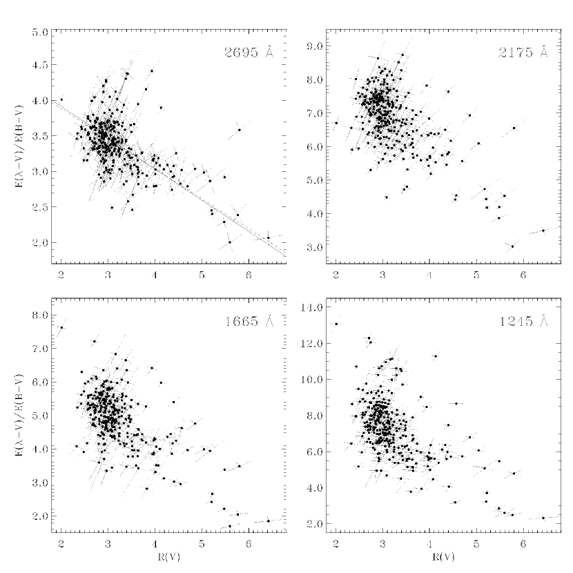
Figure 19: Plots of the measured extinction values $E(\lambda-V)/E(B-V)$ vs. $R(V)$ at four different UV wavelengths. 1-$\sigma$ error bars are shown, based on our Monte Carlo simulations as in previous figures. Any true relationships seen in plots of $A(\lambda)/A(V)$ vs. $R(V)^{-1}$ are preserved in plots of $E(\lambda-V)/E(B-V)$ vs. $R(V)$, but with the great benefit that the correlations between the errors are greatly reduced. The solid line in the 2695 Å panel is a weighted linear fit to the data, which minimizes the scatter perpendicular to the relation. This fit is $E(2695\;{\rm\AA}\;-V)/E(B-V)=4.80-0.44\;R(V)$. The nearly coincident dashed line is the fit in Figure 18 transformed by Equation (13). This fit is $E(2695\;{\rm\AA}\;-V)/E(B-V)=4.73-0.42\;R(V)$.

I.e., any true linear correlation between $A(\lambda)/A(V)$ and $R(V)^{-1}$ will also be present between $E(\lambda-V)/E(B-V)$ and $R(V)$, with a simple transformation relating the linear coefficients. The great advantage to viewing the data in the $E(\lambda-V)/E(B-V)$ vs. $R(V)$ reference frame is that no artificial correlations (in either the parameters or their uncertainties) are introduced and we only have to deal with the natural correlations which arise from the dependence of all the extinction parameters on the properties of the best-fit stellar SEDs. Figure 19 illustrates this point. It shows plots of $E(\lambda-V)/E(B-V)$ vs. $R(V)$ (along with their associated 1-$\sigma$ errors) for the same four wavelengths as in Figure 18. The 2695 Å panel shows a weighted linear fit, which is given by $E(2695\;{\rm\AA}-V)/E(B-V)=4.80-0.44\;R(V)$. This is nearly exactly what would be expected from the fit to $A(2695\;{\rm\AA})/A(V)$ vs. $R(V)^{-1}$ in Figure 18 and the transformation in Equation (13). The exact transformation is shown by the nearly coincident dashed line in Figure 19, verifying the argument leading to Equation (13). (A careful comparison between the lines and the data points will show that the two panels do indeed show the same relationship.)

From a statistical point of view, the presentations in Figures 18 and 19 are identical, as are the linear fits to the 2965 Å data. In fact, both fits have nearly identical, underwhelming, reduced $\chi^{2}$ values of $\sim$4.2. Fits performed at wavelengths shortward of 2675 Å, show increasingly large values of $\chi^{2}$ (e.g., $\chi^{2}=6.9$ for a linear fit at 1665 Å). The lesson from Figures 18 and 19 is that the choice of normalization affects the perception of how well-related $R(V)$ is to the level of UV extinction. The data in Figure 18 look better-correlated than do those in Figure 19 — but they are not. The “cosmic scatter” is appreciable and there is no functional relationship between $R(V)$ and the UV extinction (whether linear or more complex) for which the scatter approaches the current level of measurement errors. Although there is a relationship in the sense that large-$R(V)$ curves [i.e., $R(V)\gtrsim 4.0$] differ systematically from low-$R(V)$ curves, UV extinction properties cannot be expressed as a 1-parameter family in $R(V)$ at anywhere near the level of observational accuracy.

Note that the discussion above is not affected by the likelihood that some of the sightlines are composites, possibly spanning distinct regions of very different $R(V)$. If a universal relationship of the form in Equation (11) were to hold, then composite regions would still lie along the line $a(\lambda)+b(\lambda)\;R(V)^{-1}$ and would not result in “cosmic scatter.”

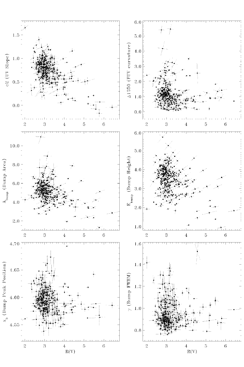
Figure 20: Plots of UV fit parameters (and derived quantities) vs. $R(V)$. 1-$\sigma$ error bars are shown, based on our Monte Carlo simulations as in previous figures. The quantity $\Delta$1250 is the difference between the observed value of $E(\lambda-V)/E(B-V)$ at 1250 Å (8.0 $\mu{\rm m}^{-1}$) and an extrapolation of the linear plus bump components of UV extinction. It thus measures the strength of the FUV curvature and is computed by $\Delta 1250=c_{4}(8.0-c_{5})^{2}$ (see Eq. [4]). $A_{bump}\equiv\pi\;c_{3}/(2\gamma)$ is the area under the 2175 Å bump. $E_{bump}\equiv c_{3}/\gamma^{2}$ is the height of the 2175 Å bump above the linear background extinction.

The recent study by Valencic et al. (2004) examined the $R(V)$-dependence of UV extinction by looking at correlations between $R(V)^{-1}$ and UV fit parameters based on the Paper III formulation, as had been done in F99 and F04. As noted earlier, they concluded that most Galactic curves (i.e., 93%) are consistent with a $R(V)$-dependent “law.” While the approach was somewhat different, the results of the Valencic et al. study suffer the same problem as shown in Figures 18 and 19 because they explicitly multiply the UV fit coefficients by $R(V)^{-1}$, thus forcing a correlation in the errors and enhancing the perception of a correlation between the quantities. The large percentage of curves believed to be consistent with a single $R(V)^{-1}$ relation results from the complications introduced by the choice of curve normalization. Figure 20 shows the relationship between $R(V)$ and the UV fitting parameters in their original form, in which the correlations among the parameters and their errors are not artificially enhanced. The figure contains several extra quantities derived from the fit parameters which help describe features of the UV curves and which are defined in §3 (and also in the figure legend). This figure again shows that, while systematic differences exist between high-$R(V)$ and low-$R(V)$ curves, there is no simple (or complex) relation between $R(V)$ and the UV fitting properties which is consistent with measurement errors.

7 SUMMARY

Several of our findings are worth emphasizing.

Variability of $x_{0}$ and $\gamma$:  We found, in accordance with our previous analysis, that while the central position of the 2175 Å bump does not vary much, it is indeed variable. On the other hand, the bump width varies considerably. Further, there still appears to be no relationship between the central position of the bump and and its width – verifying the results described in Paper I to a higher degree of accuracy than previously possible.

Correlations among the fit parameters:  Generally, the various fit parameters which describe the shape of the UV-through-IR extinction curves are not related to one another. The only exceptions are $c_{1}-c_{2}$ and $k_{IR}-R(V)$. The first relates the slope and intercept of the UV portion of the curve and is effectively a functional relationship for most of the data. The latter relates the scale factor of the power law used to describe the IR portion of the curve and the ratio of total-to-selective extinction. At the level of our measurements errors, these two parameters are functionally related and consistent with a universal form to IR extinction. However, due to observational uncertainties, the dominance of diffuse ISM sightlines in our study, and the limitations of the IR data we employ, our results are not ideal for addressing the detailed shape of IR extinction and significant sightline-to-sightline variations could still exist.

Correlations with dust density:  As determined in the past, various properties of the extinction curves are weakly correlated with the mean line of sight dust density, as measured by $E(B-V)/d$. Presumably, these correlations reflect the operation of a physical process, such as grain growth or coagulation.

Correlations of $R(V)$ with UV curve properties relationship:  Correlations between $R(V)$ and UV curve properties have received considerable attention over the years since Cardelli et al. (1988) first pointed out that a large-scale trend could be found. By expressing the curves in their native form, we verify that a there is a weak relationship between $R(V)$ and the UV in the sense that sightlines with extremely large $R(V)$ values tend to have low normalized UV extinction curves. However, this relationship is only evident for the largest $R(V)$ sightlines. For the majority of sightlines, there is no evidence for an $R(V)$-dependence of the extinction curve shapes. Specifically, inspection of Figure 19 shows that for diffuse ISM sightlines ($2.4<R(V)<3.6$), which comprise the bulk (82%) of our sample, no relationship exists, even though a large range in the extinction is present. Moreover, Figure 20 shows that the 2175 Å bump properties display a similar behavior, i.e., a trend is evident only for the largest $R(V)$ values, with the strength of the bump (as measured by $A_{bump}$ or $E_{bump}$) tending to be slightly weaker than the average for lower $R(V)$ sightlines. Thus, we conclude that there is no global 1-parameter family of extinction curves, although extremely large $R(V)$ curves tend to have distinctive properties.

Extinction curve variability – the meaning and utility of an average curve:  The previous result begs the meaning of an average extinction curve. As noted in §6.1, simple mean curves always reflect the biases of their parent samples. Our mean curve for the diffuse ISM (Figure 9, an average of all curves with $2.4\leq R(V)\leq 3.6$, and that from Valencic et al. (2004, for R=3.1) are derived from the largest samples and probably provide the best estimate of mean Galactic diffuse ISM extinction properties at short wavelengths. However, one must always be mindful of the dark shaded region in Figure 9 which illustrates the RMS variance that can be expected for an extinction curve along an arbitrary diffuse sightline. Typical RMS dispersions in $k(\lambda-V)$ are 0.31, 0.68, 0.62, 1.44 at $\lambda=$2695, 2175, 1665, 1245 Å, respectively. This means that if the mean curve is used to deredden an object with $E(B-V)=0.50$ mag, the uncertainty in the dereddened continuum at these wavelengths would be 0.15, 0.30, 0.30 and 0.72 mag, respectively, due to uncertainties in the extinction alone! It is, however, possible to take advantage of localized uniformity in the extinction to reduce this error (e.g., Massa & Savage 1981).

Physical implications:  Perhaps the best way to summarize the physical origin of the $R(V)$-dependence for Galactic extinction is to examine the $R(V)^{-1}-c_{2}$ plot shown in Figure 21, which includes a best-fit linear relation (such a relation was the basis for the $R(V)$-dependent curves produced by F99 and F04 – see Figure 10 of F04). Figure 21 can be summarized thusly: when extinction curves are steep in the optical (large $R(V)^{-1}$) they tend to stay steep in the UV (large $c_{2}$) and when extinction curves are flat in the optical (small $R(V)^{-1}$) they tend to stay flat in the UV (small $c_{2}$). However, as the scatter in the Figure illustrates, this trend is only apparent for extreme values of $R(V)^{-1}$ or $c_{2}$. In general, there is no unique relation between these parameters over the range spanned by most of the sample. It is likely that the general connection between UV and optical extinction slopes simply reflects the fact that the overall grain size distribution affects all wavelengths. But the presence of such a large scatter demonstrates that several other factors (e.g., chemical composition, grain history, coagulation, coating, radiation environment, etc.) must also be involved. In other words, the large variance in the relation between UV and optical slopes indicates that dust grain size distributions do not behave as a 1-parameter family.

Final remarks:  Having painted a negative picture of the relationship between $R(V)$ and extinction properties at other wavelengths, it would be disingenuous of us to present yet another set of $R(V)$-dependent curves. The results of Cardelli et al. (1989), F04 (which supersedes those of F99), and Valencic et al. (2004) are all reasonable, and the differences among them are instructive of the biases introduced by sample selection and methodology. It should always be remembered that these curves represent very general trends in Galactic extinction and do not constitute a standard of normalcy. Finally, although the prospect of accurately dereddening an unknown SED using a mean extinction curve is poor, this same variability demonstrates that extinction curves are responsive to local conditions, so that each one contains potentially unique information about the grains along the sightline.

Appendix A Obtaining the Data from this Study

The extinction curves and associated information from this study are available via anonymous ftp at “ftp.astronomy.villanova.edu”. After logging in as “anonymous”, change to the appropriate directory by typing “cd fitz$/$FMV_EXTINCTION”. A “README” file, two IDL procedure files, and two tar files are present. The tar files contain the extinction curves from this program and the R-dependent curves from Fitzpatrick 2004 (“FMV_EXTCURVES.tar” and “F04_RCURVES.tar”, respectively). The tar files unfold into individual ascii data files for each extinction curve, containing the 12 extinction parameters which describe the curve and the curve itself (along with 1-$\sigma$ uncertainties for the curves from this paper). The two IDL procedures provide tools for reading data from the ascii files and for constructing extinction curves from the 12 fit parameters (“READ_FMV_FILES.pro” and “MAKE_FMV_CURVE.pro”, respectively).

Table 1: Basic Data for Survey Stars [The complete version of this table is in the electronic edition of the Journal. The printed edition contains only a sample.]

Star	Spectral	V	Distance	$l$	$b$	Reference
	Type	(mag)	(pc)	($\arcdeg$)	($\arcdeg$)
HD698	B5 II: SB	7.10	1125	$117.689$	$-4.25$	1
HD3191	B1 IV:nn	8.58	1203	$121.068$	$-1.36$	2
BD+57 245 (NGC 457)	$\cdots$	9.85	2429	$126.583$	$-4.58$	$\cdots$
BD+57 252 (NGC 457)	B1 IV	9.51	2429	$126.644$	$-4.42$	2
NGC 457 Pesch 34	$\cdots$	10.61	2429	$126.646$	$-4.38$	$\cdots$
NGC 457 Pesch 13	$\cdots$	10.78	2429	$126.646$	$-4.38$	$\cdots$
NGC 457 Pesch 9	B1 V	9.83	2429	$126.646$	$-4.38$	3
Cr 463 #18	$\cdots$	10.35	0702	$127.091$	$9.20$	$\cdots$
BD+70 131 (Cr 463)	$\cdots$	10.06	0702	$127.280$	$9.17$	$\cdots$
Cr 463 #5	$\cdots$	10.37	0702	$127.264$	$9.37$	$\cdots$

References. — (1) Hiltner 1956; (2) Morgan, Code, & Whitford 1955; (3) Hoag, & Applequist 1965; (4) Maíz-Apellániz, Walborn, Galué, & Wei 2005; (5) Johnson, & Morgan 1955; (6) Slettebak 1968; (7) Schild 1965; (8) Racine 1968; (9) Morgan, Keenan, & Kellman 1943; (10) Mendoza 1956; (11) Morgan, Whitford, & Code 1953; (12) Osawa 1959; (13) Cowley, Cowley, Jaschek, & Jaschek 1969; (14) Metreveli 1968; (15) Guetter 1968; (16) Boulon, & Fehrenbach 1959; (17) Buscombe 1962; (18) Roman 1955; (19) Georgelin, Georgelin, & Roux 1973; (20) Bouigue 1959; (21) Wenzel 1951; (22) Smith 1972; (23) Penston, Hunter, & O’Neill 1975; (24) McNamara 1976; (25) Levato H., & Abt H.A.; (26) Schild, & Chaffee 1971; (27) Borgman 1960; (28) Warren, & Hesser 1977; (29) Sharpless 1952; (30) Racine 1968; (31) Crawford, Limber, Mendoza, Schulte, Steinman, & Swihart 1955; (32) Johnson, & Morgan 1953; (33) Meadows 1961; (34) Johnson 1962; (35) Hoag, & Smith 1959; (36) Barbier, & Boulon 1960; (37) Young 1978; (38) Claria 1974; (39) Feast, Thackeray, & Wesselink 1955; (40) Moffat, & Fitzgerald 1974; (41) Houk 1978; (42) Feast, Stoy, Thackeray,& Wesselink 1961; (43) Denoyelle 1977; (44) Hoffleit 1956; (45) Turner, Grieve, Herbst, & Harris 1980; (46) Morrell, Garcia, & Levato 1988; (47) Massey, & Johnson 1993; (48) Levato, Malaroda, Morrell, Garcia, & Hernandez 1991; (49) Morris 1961; (50) Hiltner, Garrison, & Schild 1969; (51) Houk, & Cowley 1975; (52) Seidensticker 1989; (53) Feast, Thackeray, & Wesselink 1957; (54) Perry, Franklin, Landolt, & Crawford 1976; (55) Schild 1970; (56) De Vaucouleurs 1957; (57) Walraven, & Walraven 1960; (58) Garrison 1967; (59) Buscombe 1969; (60) Hardie, & Crawford 1961; (61) Perry, Hill, & Christodoulou 1991; (62) Schild, Neugebauer, & Westphal 1971; (63) Schild, Hiltner, & Sanduleak 1969; (64) Levato, & Malaroda 1980; (65) Garrison, & Schild 1979; (66) Roman 1956; (67) Houk, & Smith-Moore 1988; (68) Hiltner, Morgan, & Neff 1965; (69) Walker 1957; (70) Walker 1961; (71) Stebbins, & Kron 1956; (72) Guetter 1964; (73) Hill 1970; (74) Herbig, & Spalding 1955; (75) Vrba, & Rydgren 1984; (76) Hack 1953; (77) Roman 1951; (78) Divan 1954; (79) Garrison, & Kormendy 1976; (80) Simonson 1968; (81) Blaauw, Hiltner, & Johnson 1959; (82) Pecker 1953; (83) Boulon, Duflot, & Fehrenbach 1958

Table 2: Adopted Temperature Scale for Main Sequence O Stars

Spectral	$T_{eff}$
Type	(K)
O6	$40000$
O6.5	$38500$
O7	$37000$
O7.5	$36500$
O8	$36000$
O8.5	$34750$
O9	$33500$
O9.5	$32750$
B0	$32000$

Table 3: Best-Fit Parameters for Survey Stars [The complete version of this table is in the electronic edition of the Journal. The printed edition contains only a sample.]

Star	$T_{eff}$	$\log g$	[m/H]	$v_{turb}$	$\theta_{R}$	$E(B-V)$
	(K)			$\rm(km/s)$	(mas)	(mag)
HD698	$18434\pm 499$	$3.72\pm 0.31$	$-0.18\pm 0.10$	$3.2\pm 0.5$	$0.0670\pm 0.0014$	$0.37\pm 0.01$
HD3191	$24001\pm 890$	$3.41\pm 0.28$	$-0.43\pm 0.06$	$10$	$0.0328\pm 0.0009$	$0.68\pm 0.01$
BD+57 245 (NGC 457)	$22885\pm 697$	$3.64\pm 0.20$	$-0.39\pm 0.08$	$5.5\pm 0.6$	$0.0160\pm 0.0004$	$0.50\pm 0.01$
BD+57 252 (NGC 457)	$24924\pm 616$	$3.64\pm 0.16$	$-0.47\pm 0.06$	$10$	$0.0173\pm 0.0004$	$0.51\pm 0.01$
NGC 457 Pesch 34	$23594\pm 661$	$3.91\pm 0.17$	$-0.07\pm 0.06$	$1.2\pm 0.8$	$0.0110\pm 0.0003$	$0.51\pm 0.01$
NGC 457 Pesch 13	$22023\pm 809$	$3.84\pm 0.17$	$-0.47\pm 0.11$	$2.1\pm 0.8$	$0.0114\pm 0.0003$	$0.51\pm 0.01$
NGC 457 Pesch 9	$25738\pm 577$	$3.77\pm 0.16$	$-0.75\pm 0.07$	$9.1\pm 0.7$	$0.0147\pm 0.0003$	$0.54\pm 0.01$
Cr 463 #18	$11891\pm 286$	$3.99\pm 0.16$	$-0.60\pm 0.10$	$\mathrm{𝟎}$	$0.0198\pm 0.0003$	$0.35\pm 0.01$
BD+70 131 (Cr 463)	$11351\pm 204$	$3.93\pm 0.17$	$-0.73\pm 0.07$	$5.1\pm 0.4$	$0.0210\pm 0.0003$	$0.28\pm 0.01$
Cr 463 #5	$11859\pm 230$	$4.10\pm 0.19$	$-0.59\pm 0.09$	$2.0\pm 0.4$	$0.0170\pm 0.0002$	$0.30\pm 0.01$

Table 4: Best-Fit Extinction Curve Parameters for Survey Stars [The complete version of this table is in the electronic edition of the Journal. The printed edition contains only a sample.]

	UV Coefficients								Optical Spline Points				IR Coefficients
Star	$x_{0}$	$\gamma$	$c_{1}$	$c_{2}$	$c_{3}$	$c_{4}$	$c_{5}$		$O_{1}$	$O_{2}$	$O_{3}$		$R(V)$	$k_{IR}$
HD698	$4.551\pm 0.006$	$0.96\pm 0.03$	$0.07\pm 0.19$	$0.99\pm 0.05$	$2.95\pm 0.19$	$0.15\pm 0.05$	$6.51\pm 0.29$		$2.38\pm 0.09$	$1.33$	$0.00$		$3.94\pm 0.16$	$1.70\pm 0.18$
HD3191	$4.636\pm 0.003$	$0.94\pm 0.02$	$-0.79\pm 0.20$	$1.00\pm 0.04$	$2.99\pm 0.16$	$0.31\pm 0.02$	$5.76\pm 0.09$		$2.04\pm 0.06$	$1.33$	$0.01$		$2.81\pm 0.09$	$0.93\pm 0.14$
BD+57 245 (NGC 457)	$4.561\pm 0.005$	$0.89\pm 0.03$	$-0.47\pm 0.31$	$0.88\pm 0.06$	$3.13\pm 0.19$	$0.24\pm 0.03$	$5.71\pm 0.16$		$2.05\pm 0.06$	$1.31$	$0.00$		$2.97\pm 0.13$	$0.96\pm 0.17$
BD+57 252 (NGC 457)	$4.577\pm 0.005$	$0.92\pm 0.02$	$-0.66\pm 0.25$	$0.95\pm 0.05$	$3.39\pm 0.17$	$0.17\pm 0.02$	$5.48\pm 0.23$		$2.15\pm 0.06$	$1.32$	$0.00$		$2.97\pm 0.10$	$0.98\pm 0.15$
NGC 457 Pesch 34	$4.579\pm 0.003$	$0.91\pm 0.01$	$-0.55\pm 0.20$	$0.86\pm 0.04$	$3.32\pm 0.11$	$0.31\pm 0.02$	$6.14\pm 0.09$		$1.99\pm 0.07$	$1.30$	$0.01$		$2.94\pm 0.11$	$0.84\pm 0.16$
NGC 457 Pesch 13	$4.587\pm 0.004$	$0.87\pm 0.02$	$-0.69\pm 0.33$	$0.84\pm 0.07$	$2.91\pm 0.14$	$0.26\pm 0.02$	$5.59\pm 0.17$		$2.03\pm 0.07$	$1.31$	$0.01$		$3.11\pm 0.11$	$0.90\pm 0.16$
NGC 457 Pesch 9	$4.578\pm 0.006$	$1.07\pm 0.03$	$-1.13\pm 0.22$	$1.08\pm 0.04$	$4.31\pm 0.22$	$0.18\pm 0.02$	$5.00\pm 0.18$		$2.37\pm 0.05$	$1.35$	$0.01$		$2.76\pm 0.07$	$0.79\pm 0.12$
Cr 463 #18	$4.606\pm 0.009$	$1.18\pm 0.05$	$-0.47\pm 0.26$	$1.03\pm 0.07$	$5.23\pm 0.45$	$0.30\pm 0.03$	$5.09\pm 0.20$		$\cdots$	$1.37$	$0.01$		$3.38\pm 0.17$	$1.29$
BD+70 131 (Cr 463)	$4.577\pm 0.011$	$1.11\pm 0.05$	$0.17\pm 0.32$	$0.86\pm 0.08$	$5.11\pm 0.49$	$0.35\pm 0.04$	$5.00\pm 0.19$		$\cdots$	$1.37$	$0.00$		$3.40\pm 0.20$	$1.30$
Cr 463 #5	$4.610\pm 0.008$	$1.08\pm 0.04$	$0.45\pm 0.33$	$0.74\pm 0.08$	$4.77\pm 0.34$	$0.32\pm 0.03$	$5.06\pm 0.18$		$\cdots$	$1.37$	$0.00$		$2.91\pm 0.18$	$0.99$

Table 5: Extinction Curve Parameters for Mean Curve in Figure 9

Parameter	Value
$x_{0}$	string4.592 $\mu{\rm m}^{-1}$
$\gamma$	string0.922 $\mu{\rm m}^{-1}$
$c_{1}$	$-0.175$
$c_{2}$	string0.807
$c_{3}$	string2.991
$c_{4}$	string0.319
$c_{5}$	string6.097
$O_{1}$	string2.055
$O_{2}$	string1.322
$O_{3}$	string0.000
$R(V)$	string3.001
$k_{IR}$	string1.057

Figure 6: UV spectra of two survey stars, HD228969 and BD+54 973, compared with three early-type spectral classification standard stars. The reddened survey stars are classified as types B2 II: and B3 V, respectively, although the SED-fitting procedure indicates temperatures in the neighborhood of 30000 K. Comparison of the UV spectral features with the classification standards indicates that these two stars are likely misclassified members of earlier spectral classes. Much of the scatter in the $T_{\rm eff}$ vs. spectral type diagram in Figure 5 is probably the result of such classification uncertainties.

Figure 7: $T_{\rm eff}$ as a function of the Strömgren reddening-free index $[c]\equiv c_{1}-0.20(b-y)$, which measures the strength of the Balmer jump, for 162 sample stars. Symbols are the same as for Figure 5, with the addition of the open circles which denote O-type stars. Also shown are the spectral type vs. $T_{\rm eff}$ calibrations from Figure 5, transformed into the $T_{\rm eff}$ vs. $[c]$ plane using Crawford’s (1978) spectral type vs. $c_{0}$ and $c_{0}$ vs. $(b-y)_{0}$ relations. Note that Strömgren photometry was not used in modeling the SEDs of our survey stars.

Figure 10: Unweighted mean UV extinction curve for 318 survey stars (open circles). Ten stars (HD14092, BD+56 501, HD14321, HD18352, HD25443, CD-42 4819, HD99872, HD326328, HD197702, and HD239710) were excluded from the mean because they have incomplete IUE spectra. The individual data points (shown in Figure 4) are typically 10 Å apart. The solid curve is a parametrized fit to the mean curve, using the formulation discussed in §3. The $O-C$ residuals are shown as filled points; they are offset from their zero mean for display. A number of distinct features are seen in the residuals and labeled in the figure. These arise from ISM gas-phase absorption lines, mismatch between the C iv $\lambda$1550 stellar wind lines in the O stars and the static model SEDs, and known inadequacies in the ATLAS9 opacity distribution functions (labeled “b” in the figure; see Paper IV). No other credible features are seen in the residuals. The standard deviation of the residuals about their mean value of zero (excluding the labeled points) is $0.06\mbox{$E(B\!-\!V)$}$ mag, corresponding to $\sim 0.02A(V)$ mag. This figure demonstrates both the intrinsic smoothness of UV extinction and the ability of our parametrization scheme to reproduce the shape of UV extinction curve to extremely high accuracy.

Figure 13: Plot of the slope $c_{2}$ vs. the intercept $c_{1}$ for the linear component of UV extinction. The uncertainties in $c_{1}$ and $c_{2}$ are strongly correlated, as indicated by the 1-$\sigma$ error bars (dotted lines). The orientation of the error bars was determined by fitting ellipses to the loci of results from the Monte Carlo error simulations. The individual sets of error bars are not orthogonal to each other because the scales of the x- and y-axes are different. The solid line is a weighted linear fit to the data, designed to minimize the residuals in the direction perpendicular to the fit. It is given by $c_{1}=2.09-2.84c_{2}$.

Figure 14: Plot of $R(V)$ vs. the IR scale factor $k_{IR}$ (see Eq. [6]). The uncertainties in $R(V)$ and $k_{IR}$ are strongly correlated, as indicated by the 1-$\sigma$ error bars (dotted lines). The orientation of the error bars was determined by fitting ellipses to the loci of results from the Monte Carlo error simulations. The solid line is a weighted linear fit to the data, designed to minimize the residuals in the direction perpendicular to the fit. It is given by $k_{IR}=-0.83+0.63R(V)$.

Figure 15: Plot of $E(V-K)/E(B-V)$ vs. $R(V)$ for sightlines with 2MASS $K$-band photometry (filled circles) and Johnson $K$-band photometry (open circles). The dotted line shows the widely-used relation $R(V)=1.1E(V-K)/E(B-V)$. The solid line is a linear fit to the 2MASS data, minimizing the residuals in the direction perpendicular to the fit. It is given by $R(V)=-0.26+1.19E(V-K)/E(B-V)$.

Figure 16: Plot of the FWHM of the 2175 Å bump $\gamma$ vs. its central position, $x_{0}$, both in units of $\mu{\rm m}^{-1}$. Dotted lines show the 1-$\sigma$ error bars, revealing the uncertainties in $\gamma$ and $x_{0}$ to be generally uncorrelated. The orientation of the error bars was determined by fitting ellipses to the loci of results from the Monte Carlo error simulations. The individual sets of error bars are not orthogonal to each other because the scales of the x- and y-axes are different. A number of sightlines which deviate most from the main distribution have been labeled.

Figure 21: Plot of the slope of the UV linear component $c_{2}$ vs. $R(V)^{-1}$. 1-$\sigma$ error bars are shown, based on our Monte Carlo simulations as in previous figures. The solid line is a weighted linear fit which minimizes the residuals in the direction perpendicular to the fit. It is given by $R(V)^{-1}=0.17+0.20\;c_{2}$.

References

- Balona & Crampton (1974) Balona, L., & Crampton, D. 1974, MNRAS, 166, 203
- (2) Barbier, M., & Boulon, J. 1960, J. Obs., 43, 69
- Blaauw (1963) Blaauw, A. 1963, in Basic Astronomical Data, ed. K.A. Strand (University of Chicago Press: Chicago), Chapter 20
- (4) Blaauw, A., Hiltner, W.A., & Johnson, H.L. 1959, ApJ, 130, 69
- Bohlin (1996) Bohlin, R. C. 1996, AJ, 111, 1743
- Böhm-Vitense (1981) Böhm-Vitense, E. 1981, ARA&A, 19, 295
- (7) Borgman, J. 1960, Bull. Astron. Inst. Netherlands, 15, 255
- (8) Bouigue, M.R. 1959, Publ. Obs. Haute-Provence, 4, 52
- (9) Boulon, J., Duflot, M., & Fehrenbach, C. 1958, J. Obs., 42, 1
- (10) Boulon, J., & Fehrenbach, C. 1959, Publ. Obs. Haute-Provence, 4, 55
- (11) Buscombe, W. 1962, Mount Stromlo Obs. Mimeo., 4, 1
- (12) Buscombe, W. 1969, MNRAS, 144, 31
- Cardelli et al. (1988) Cardelli, J.A., Clayton, G.C. & Mathis, J.S. 1988, ApJ, 329, 33
- Cardelli et al. (1989) Cardelli, J.A., Clayton, G.C. & Mathis, J.S. 1989, ApJ, 345, 245
- Cardelli et al. (1992) Cardelli, J.A., Sembach, K.R., & Mathis, J.S. 1992, AJ, 104, 1916
- Chini and Krügel (1983) Chini, R. & Krügel, E. 1983, A&A, 117, 289
- (17) Claria, J.J. 1974, AJ, 79, 1022
- Clayton & Fitzpatrick (1987) Clayton, G.C., & Fitzpatrick, E.L. 1987, AJ, 92, 147
- Clayton et al. (2000) Clayton, G.C., Gordon, K.D., & Wolff, M.J. 2000, ApJS, 129, 147
- Clayton et al. (2003) Clayton, G.C., et al. 2003, ApJ, 592, 947
- (21) Cowley, A., Cowley, C., Jaschek, M., & Jaschek, C. 1969, AJ, 74, 375
- Crawford (1978) Crawford, D.L. 1978, AJ, 83, 48
- Crawford & Barnes (1970) Crawford, D.L., & Barnes, J.V. 1970, AJ, 75, 952
- (24) Crawford, D., Limber, D.N., Mendoza, E.E., Schulte, D., Steinman, H., & Swihart, T. 1955, ApJ, 121, 24
- (25) De Vaucouleurs, A. 1957, MNRAS, 117, 449
- (26) Denoyelle, J. 1977, A&AS, 27, 343
- (27) Divan, L. 1954, Annales d’Astrophysique, 17, 456
- Draine (2003) Draine, B.T. 2003, ARA&A, 41, 241
- (29) Feast, M.W., Stoy, R.H., Thackeray, A.D., & Wesselink, A.J. 1961, MNRAS, 122, 239
- (30) Feast, M.W., Thackeray, A.D., & Wesselink, A.J. 1955, Mem. R. Astron. Soc, 67, 51
- (31) Feast, M.W., Thackeray, A.D., & Wesselink, A.J. 1957, Mem. R. Astron. Soc, 68, 1
- Fitzpatrick (1999) Fitzpatrick, E.L. 1999, PASP, 111, 63 (F99)
- Fitzpatrick (2004) Fitzpatrick, E.L. 2004, in Astrophysics of Dust, eds. A.N. Witt, G.C. Clayton, & B.T. Draine, ASP Conference Series, Vol. 309, 33 (F04)
- Fitzpatrick & Massa (1986) Fitzpatrick, E.L., & Massa D. 1986, ApJ, 307, 286 (Paper I)
- Fitzpatrick & Massa (1988) Fitzpatrick, E.L., & Massa D. 1988, ApJ, 328, 734 (Paper II)
- Fitzpatrick & Massa (1990) Fitzpatrick, E.L., & Massa D. 1990, ApJS, 72, 163 (Paper III)
- Fitzpatrick & Massa (1999) Fitzpatrick, E.L., & Massa D. 1999, ApJ, 525, 1011
- (38) Fitzpatrick, E.L., & Massa D. 2005a, AJ, 130, 1127 (Paper IV)
- (39) Fitzpatrick, E.L., & Massa D. 2005b, AJ, 129, 1642
- Flower (1977) Flower, P.J. 1977, A&A, 54 31
- (41) Garrison, R.F. 1967, ApJ, 147, 1003
- (42) Garrison, R.F., & Kormendy, J. 1976, PASP, 88, 865
- (43) Garrison, R.F., & Schild, R.E. 1979, AJ, 84, 1020
- Georgelin & Georgelin (1976) Georgelin, Y.M., & Georgelin, Y.P. 1976, A&AS, 49, 57
- (45) Georgelin, Y.M., Georgelin, Y.P., & Roux, S. 1973, A&A, 25, 337
- (46) Guetter, H.H. 1964, Publications of the David Dunlap Observatory, 2, 403
- (47) Guetter, H.H. 1968, PASP, 80, 197
- (48) Hack, M. 1953, Annales d’Astrophysique, 16, 417
- (49) Hardie R.H., & Crawford, D.L. 1961, ApJ, 133, 843
- (50) Herbig, G.H., & Spalding, J. 1955, ApJ, 121, 118
- (51) Hill, P.W. 1970, MNRAS, 150, 23
- (52) Hiltner, W.A. 1956, ApJS, 2, 389
- (53) Hiltner, W.A., Garrison R.F., & Schild R.E. 1969, ApJ, 157, 313
- (54) Hiltner, W.A., Morgan, W.W., & Neff, J.S. 1965, ApJ, 141, 183
- (55) Hoag, A.A., & Applequist, N.L. 1965, ApJS, 12, 215
- (56) Hoag, A.A., & Smith, E.V.P. 1959, PASP, 71, 32
- (57) Hoffleit, D. 1956, ApJ, 124, 61
- (58) Houk N., & Cowley, A.P. 1975, Michigan Catalogue of Two-Dimensional Spectral Types for the HD Stars, C01, 0
- (59) Houk, N. 1978, Michigan Catalogue of Two-Dimensional Spectral Types for the HD Stars, C02, 0
- (60) Houk, N., & Smith-Moore, M. 1988, Michigan Catalogue of Two-Dimensional Spectral Types for the HD Stars, C04, 0
- Humphreys & McElroy (1984) Humphreys, R.M. & McElroy, D.B. 1984, ApJ, 284, 565
- (62) Johnson, H.L. 1962, ApJ, 136, 1135
- Johnson (1968) Johnson, H.L. 1968, in Nebulae and Interstellar Matter, eds. B.M. Middlehurst & L.H. Aller (University of Chicago Press: Chicago), Chapter 5
- (64) Johnson, H.L., & Morgan, W.W. 1953, ApJ, 117, 313
- (65) Johnson, H.L., & Morgan, W.W. 1955, ApJ, 122, 429
- Kiszkurno-Koziej & Lequeux (1987) Kiszkurno-Koziej, E. & Lequeux, J. 1987, A&A, 185, 291
- Kurucz (1991) Kurucz, R.L. 1991, in Stellar Atmospheres: Beyond Classical Models, ed. L. Crivellari, I. Hubeny, & D. G. Hummer (NATO ASI Ser. C.; Dordrect: Reidel), 441
- Lanz & Hubeny (2003) Lanz, T., & Hubeny, I. 2003, ApJS, 146, 417
- Larson & Whittet (2005) Larson, K.A., & Whittet, D.C.B. 2005, ApJ, 623, 897
- Levato & Abt (1976) Levato, H., & Abt, H.A. 1976 PASP, 88, 712
- (71) Levato H., & Malaroda S. 1980, PASP, 92, 323
- (72) Levato, H., Malaroda, S., Morrell, N., Garcia, B., & Hernandez, C. 1991, ApJS, 75, 869
- (73) Maíz-Apellániz, J., Walborn, N.R., & Galué, H.A., Wei L. 2004, ApJS, 151, 103
- Malagnini et al. (1984) Malagnini, M.L., Morossi, C., & Faraggiana, R. 1984, in The MK Process and Stellar classification, ed. R.F. Garrison (David Dunlap Observatory:Toronto), 321 375
- Martin & Whittet (1990) Martin, P.G., & Whittet, D.C.B. 1990, ApJ, 357, 113
- Martins, Schaerer, & Hillier (2005) Martins, F., Schaerer, D., & Hillier, D.J. 2005, A&A, 436,1049
- Massa (1987) Massa, D. 1987, AJ, 94, 1675
- Massa & Fitzpatrick (1986) Massa, D., & Fitzpatrick, E.L. 1986, ApJS, 60, 305
- Massa & Fitzpatrick (2000) Massa, D., & Fitzpatrick, E.L. 2000, ApJS, 126, 517 (MF00)
- Massa & Savage (1981) Massa, D., & Savage, B.D. 1981, ApJ, 248, 201
- Massa & Savage (1984) Massa, D., & Savage, B.D. 1984, ApJ, 279, 310
- Massa et al. (1983) Massa, D., Savage, B.D., & Fitzpatrick, E.L. 1983, ApJ, 266, 662
- (83) Massey, P., & Johnson, J., 1993, AJ, 105, 980
- (84) McNamara, B.J. 1976, AJ, 81, 375
- (85) Meadows, A.J. 1961, MNRAS,123, 81
- (86) Mendoza, E.E. 1956, ApJ, 123, 54
- Mermilliod et al., (1997) Mermilliod, J.-C., Mermilliod, M., & Hauck, B. 1997 A&AS, 124, 349
- (88) Metreveli, M.D. 1968, Abastumanskaya Astrofiz. Obs., Byull., 38, 93
- (89) Moffat, A.F.J., & Fitzgerald, M.P. 1974, A&A, 34, 291
- Morgan et al. (1982) Morgan, D.H., McLachlan, A., & Nandy, K. 1982, MNRAS, 198, 779
- (91) Morgan, W.W., Code, A.D., & Whitford, A.E. 1955, ApJS, 2, 41
- (92) Morgan, W.W., Keenan, P.C., & Kellman, E. 1943, An Atlas of Stellar Spectra, With an Outline of Spectral Classification (University of Chicago Press:Chicago)
- (93) Morgan, W.W., Whitford, A.E., & Code, A.D. 1953, ApJ, 118, 318
- (94) Morrell, N., Garcia, B., & Levato, H. 1988, PASP, 100, 1431
- (95) Morris, P.M. 1961, MNRAS, 122, 325
- Nichols & Linsky, (1996) Nichols, J.S. & Linsky, J.L. 1996, AJ, 111, 517
- Nishiyama et al. (2006) Nishiyama, S., et al. 2006, ApJ, 638, 846
- (98) Osawa, K. 1959, ApJ, 130, 159
- Panagia (1973) Panagia, N. 1973, AJ, 78, 929
- Panek (1983) Panek, R.J. 1983,ApJ, 270, 169
- (101) Pecker, Ch. 1953, Annales d’Astrophysique, 16, 321
- (102) Penston, M.V., Hunter, J.K., & O’Neill, T. 1975, MNRAS, 171, 219
- Perez et al. (1987) Perez, M.R., The, P.S., & Westerlund, B.E., 1987, PASP, 99, 1050
- (104) Perry C.L., Hill, G., & Christodoulou, D.M. 1991, A&AS, 90, 195
- (105) Perry, C.L., Franklin, C.B., Landolt, A.U., & Crawford D.L. 1976, AJ, 81, 632
- Rachford et al (2002) Rachford, B.L., et al. 2002, ApJ, 577, 221
- (107) Racine, R. 1968, AJ, 73, 233
- (108) Racine, R., 1968, AJ, 73, 588
- (109) Roman, N.G. 1951, ApJ, 114, 492
- (110) Roman, N.G. 1955, ApJS, 2, 195
- (111) Roman, N.G. 1956, ApJ, 123, 246
- Rosenzweig & Morrison (1986) Rosenzweig, P., & Morrison, N.D. 1986, ApJ, 306, 522
- Savage & Mathis (1979) Savage, B.D., & Mathis, J.S. 1979, ARA&A, 17, 73
- Savage et al. (1985) Savage, B.D., Massa, D., Meade, M., Wesselius, P.R. 1985, ApJS,59, 397
- (115) Schild R., Neugebauer, G., & Westphal, J.A. 1971, AJ, 76, 237
- (116) Schild R.E., Hiltner, W.A., & Sanduleak, N., 1969 ApJ, 156, 609
- (117) Schild, R.E. 1970, ApJ, 161, 855
- (118) Schild, R.E., 1965 ApJ, 142, 979
- (119) Schild, R.E., & Chaffee, F. 1971, ApJ, 169, 529
- Schmidt-Kaler (1982) Schmidt-Kaler, Th. 1982, in Landolt-Bornstein, Numerical Data and Functional Relationships in Science and Technology, Vol. 2, eds. K. Schaifers & H.H. Voigt (Springer Verlag:Berlin), 451
- Seaton (1979) Seaton, M.J. 1979, MNRAS, 187, 73P
- (122) Seidensticker, K.J. 1989, A&AS, 79, 61
- (123) Sharpless, S. 1952, ApJ, 116, 251
- (124) Simonson, S.C. 1968, ApJ, 154, 923
- (125) Slettebak, A., 1968 ApJ, 154, 933
- (126) Smith, M.A. 1972, ApJ, 175, 765
- (127) Stebbins, J., & Kron, G.E. 1956, ApJ, 123, 440 Tapia, M.; Roth, M.; Marraco, H.; Ruiz, M. T. Royal Astronomical Society, Monthly Notices (ISSN 0035-8711), vol. 232, June 1, 1988, p. 661-681
- Torres (1987) Torres, A.V. 1987, ApJ, 322, 949
- Turner (1980) Turner, D.G. 1980, ApJ, 240, 137
- (130) Turner, D.G., Grieve, G.R., Herbst, W., & Harris, W.E. 1980, AJ, 85, 1193
- Valencic et al. (2004) Valencic, L.A., Clayton, G.C., & Gordon, K.D. 2004, ApJ, 616, 912
- (132) Vrba, F.J., & Rydgren, A.E. 1984, ApJ, 283, 123
- Walborn & Fitzpatrick (1990) Walborn, N.R., & Fitzpatrick, E.L. 1990, PASP, 102, 379
- (134) Walker, M.F. 1957, ApJ, 125, 636
- (135) Walker, M.F. 1961, ApJ, 133, 438
- (136) Walraven, T., & Walraven, J.H. 1960, Bull. Astron. Inst. Netherlands, 15, 67
- (137) Warren, W.H., & Hesser J.E. 1977, ApJS, 34, 115
- (138) Wenzel, W. 1951, Veroeff. Sternwarte Sonneber, 5, 1
- Wu et al. (1980) Wu, C.-C., Gilra, D.P., & van Duinen, R.J. 1980, ApJ, 241, 173
- (140) Young, A. 1978, PASP, 90, 144