Quantitative relations between corruption and economic factors

Abstract

We report quantitative relations between corruption level and economic factors, such as country wealth and foreign investment per capita, which are characterized by a power law spanning multiple scales of wealth and investments per capita. These relations hold for diverse countries, and also remain stable over different time periods. We also observe a negative correlation between level of corruption and long-term economic growth. We find similar results for two independent indices of corruption, suggesting that the relation between corruption and wealth does not depend on the specific measure of corruption. The functional relations we report have implications when assessing the relative level of corruption for two countries with comparable wealth, and for quantifying the impact of corruption on economic growth and foreign investments.

1 Introduction

Corruption influences important aspects of social and economic life. The level of corruption in a given country is widely believed to be an important factor to consider when projecting economic growth, estimating the effectiveness of the government administration, making decisions for strategic investments, and forming international policies. The relation between corruption level and key parameters of economic performance is largely qualitative SA1 ; MAURO ; IMF ; LEFF ; HUNT ; WHEE ; HINE ; WEI . Corruption has become increasingly important with the globalization of the international economic and political relations between countries, which has led various governmental and non-governmental organizations to search for adequate measures to quantify levels of corruption SA1 ; MAURO ; KKM ; KK ; TREI ; jain .

Systematic studies of corruption have been hampered because of the complexity and secretive nature of corruption, making it difficult to quantify. There have been concerted efforts to introduce quantitative measures suitable for describing levels of corruption across diverse countries CI ; CPI ; CC . However, a specific functional dependence between quantitative measures of corruption and economic performance has not been established.

Previous studies have suggested a negative association between corruption level and country wealth SA1 ; MAURO ; IMF . There is active debate concerning the relation between corruption level and economic growth BARD ; lambs . Some earlier studies suggest that corruption may help the most efficient firms bypass bureaucratic obstacles and rigid laws LEFF ; HUNT leading to a positive effect on economic growth, while more recent works do not find a significant negative dependence between corruption and growth SA1 ; MAURO . Further, studies of net flow of foreign investment report conflicting results. Some studies find no significant correlation between inward foreign investment and corruption level in host countries WHEE ; HINE , while others indicate a negative association between corruption and foreign investments MAURO ; WEI . This debate reflects the inherent complexity of the problem as countries in the world vary dramatically in their social and economic development SCHN . Thus, an open question remains whether there is a general functional relation between corruption level and key aspects of the economic performance of different countries.

We develop and test the hypothesis that there may be a power-law dependence between corruption level and economic performance which holds across diverse countries regardless of differences in specific country characteristics such as country wealth (defined in our paper as gross domestic product per capita) or foreign direct investment. Recent studies show that diverse social and economic systems exhibit scale invariant behavior — e.g., size ranking and growth of firms, universities, urban centers, countries and even people’s personal fortunes follow a power law over a broad range of scales MAKSE ; AXTELL ; MST ; YKL ; FDF ; UNIVER ; IVANOV ; NEWMAN . Since countries in the world greatly differ in their wealth and foreign investments, we test the possibility that there may be an underlying organization, such that the cross-country relations between corruption level and country wealth, and corruption level and foreign investments exhibit a significant negative correlation characterized by scale-invariant properties over multiple scales, and thus they can be described by power laws. Specifically, we test if this scale-invariant behavior remains stable over different time periods, as well as its validity for different subgroups of countries. Finally, we demonstrate a strong correlation between corruption level and past long-term economic growth.

2 Data and Methods

We analyze the Corruption Perceptions Index (CPI) CPI ; method introduced by Transparency International CPI , a global civil organization supported by a wide network of government agencies, developmental organizations, foundations, public institutions, the private sector, and individuals. The CPI is a composite index based on independent surveys of business people and on assessments of corruption in different countries provided by more than ten independent institutions around the world, including the World Economic Forum, United Nations Economic Commission for Africa, the Economist Intelligence Unit, the International Institute for Management Development method . The CPI spans 10-year period 1996-2005. The different surveys and assessments use diverse sampling frames and different methodologies. Some of the institutions consult a panel of experts to assess the level of corruption, while others, such as the International Institute for Management Development and the Political and Economic Risk Consultancy, turn to elite businessmen and businesswomen from different industries. Further, certain institutions gather information about the perceptions of corruption from residents with respect to the performance of their home countries, while other institutions survey the perceptions of non-residents in regard to foreign countries or specifically in regard to neighboring countries. All sources employ a homogeneous definition of corruption as the misuse of public power for private benefit, such as bribing public officials, kickbacks in public procurement, or embezzlement of public funds. Each of these sources also assesses the “extent” of corruption among public officials and politicians in different countries. Transparency International uses non-parametric statistics for standardizing the data and for determining the precision of the scores method . While there is a certain subjectivity in people’s perceptions of corruption, the large number of independent surveys and assessments based on different methodologies averages out most of the bias. The CPI ranges from 0 (highly corrupt) to 10 (highly transparent).

We also analyze a different measure of corruption, the Control of Corruption Index (CCI) KKM ; CC provided by the World Bank CC . The CCI ranges from –2.5 to 2.5, with positive numbers indicating low levels of corruption. As a measure of country wealth, we use the gdp, defined to be the annual nominal gross domestic product per capita in current prices in U.S. dollars, provided by the International Monetary Fund (IMF) IMFGDP over the 26-year period 1980-2005. As a measure of foreign direct investment we use annual data from the Bureau of Economic Analysis BEA of the United States (U.S.) government, which represents the direct investment received by different countries from the U.S. over the period 2000-2004. These data are appropriate for our study since (i) the U.S. has been the dominant source of foreign investment in the past decades and (ii) the 1977 Foreign Corrupt Practices Act (FCPA) FCPA holds U.S. companies legally liable for bribing foreign government officials, which makes the U.S. a source country which penalizes its multinational companies for corruption practices WEI .

3 Results and Discussion

3.1 Relation Between Corruption Level and Country Wealth.

To test if there is a common functional dependence between corruption level and country wealth, we plot the CPI versus gdp for different countries [Fig. 1(a-e)]. We find a positive correlation between CPI and country wealth, which can be well approximated by a power law

$$CPI\sim({\it gdp})^{\mu},$$ (1)

where $\mu>0$, indicating that richer countries are less corrupt. Most countries fall close to the power-law fitting line shown in Fig. 1, consistent with specific functional relation between corruption and country wealth even for countries characterized by levels of wealth ranging over a factor of $10^{3}$. This finding in Eq. (1) indicates that the relative corruption level between two countries should be considered not only in terms of CPI values but also in the context of country wealth. For example, two countries with a large difference in their gdp on average will not have the same level of corruption, as our results quantify the degree to which poorer countries with lower gdp have higher levels of corruption.

The quantitative relation between CPI and gdp for all countries in the world — represented by the power-law fitting curves in Fig. 1 — indicates where is the “expected” level of corruption for a given level of wealth. A country above (or below) the fitting line is less (or more) corrupt than expected for its level of wealth. For example, comparing the relative corruption level of two countries with similar gdp such as Bulgaria and Romania, one can assess that Bulgaria is less corrupt than Romania [Fig. 3]. Depending whether a specific country is above (e.g., Bulgaria) or below (e.g., Romania) the power-law fit, one can assess if this country is less (or more) corrupt relative to the average level of corruption corresponding to the wealth of this country.

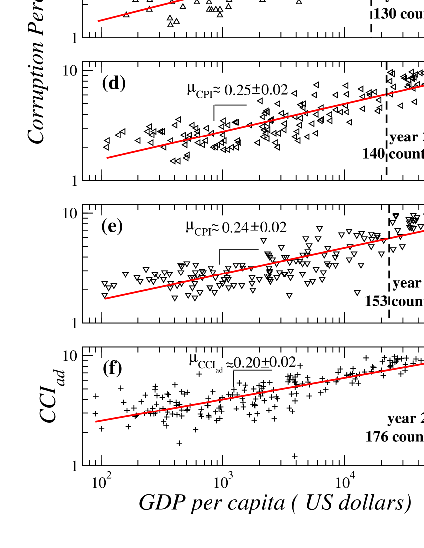
Figure 1: Log-log plots of the corruption perceptions index (CPI) versus GDP per capita (gdp) indicating a power-law functional dependence. A low value of CPI corresponds to a high level of corruption CPI . Data on gdp are obtained as current prices in U.S. dollars IMFGDP . (a)-(e) The power-law functional dependence remains stable over different time periods, and is characterized by similar values of the exponent $\mu$ for different years and different number of countries. The power-law fit indicates the expected level of corruption expected for given country wealth. Note that, comparing two countries with a similar gdp, the country placed above the power-law fit is less corrupt than one would expect for its level of wealth, while the country below the power-law curve has a relatively higher level of corruption than one would expect for its wealth. (f) We obtain similar results for the adjusted control of corruption index $CCI_{ad}$ CC , which is independent of CPI, indicating that the scale-invariant relation between corruption and wealth does not depend on the specific measure of corruption. Vertical dashed lines in the panels seperate the top 30 wealthiest countries. (see Fig. 5 and Fig. 6)

Moreover, the quantitative dependence we find in Eq. (1) allows us to compare the relative levels of corruption between two countries which belong to two different wealth brackets. Specifically, two countries with a very different gdp should not be compared only by the value of their CPI, but also by their relative distances from the power-law fitting line which indicates the expected level of corruption. For example, Bulgaria and Slovenia differ significantly in their wealth (Slovenia has $\approx 5$ times higher gdp), but both countries are at equal distances above the fitting line, indicating (i) that both countries are less corrupt than the corruption level expected for their corresponding wealth and (ii) that the relative level of corruption of Slovenia within the group of countries falling in the same gdp bracket as Slovenia is similar to the relative corruption level of Bulgaria within the group of countries falling in the same gdp bracket as Bulgaria [Fig. 3].

To test how robust is the power-law dependence between corruption and country wealth, we analyze groups containing different numbers of countries, and we find that Eq. (1) holds, with similar values of $\mu$ [Fig. 1(a-e)]. Averaging the power-law exponent $\mu$ for different years and for different number of countries we find $\overline{\mu}\approx$0.27$\pm\Delta$, where $\Delta$=0.02 is the standard deviation. For the CPI and gdp data we find an average correlation coefficient of 0.86. We also note that the inverse relation of gdp as a function of CPI is characterized by an exponent $\hat{\mu}$ which is not equal to 1/$\mu$ as one might expect, since the correlation coefficient of the data fit is less than 1. Next, we analyze data comprising the same set of countries for different years [Fig. 2], and we find that the power-law dependence of Eq. (1) remains stable in time over periods shorter than a decade, with similar and slightly decreasing values for $\mu$ [Fig. 1 and Fig. 2]. Similar results we obtain also for the period 1996-2000 (not shown in the figures as available data cover much smaller number of countries for that period).

Given the facts that (i) the number of countries we analyze changes from 90 to 153, and (ii) that the time horizon of 5-6 years we consider could be sufficient for significant changes in both corruption level and wealth (e.g., the case of Eastern European countries), our finding of a power-law relationship in Eq. (1) is consistent with a universal dependence between gdp and CPI across diverse countries. We note that the power-law relation in Eq. (1) holds when gdp is calculated both as current prices in US dollars [Fig. 1 and Fig. 2], as well as the value based on purchasing power parity [Fig. 4]. Further, Eq. (1) implies that lowering the corruption level of a country would lead to an increase in its gdp and vice versa—e.g., for a country with gdp $\approx\$4000$ an increase in CPI of 0.25 units would lead to increase in the gdp of approximately $\$700$ [Fig. 1 and Fig. 2].

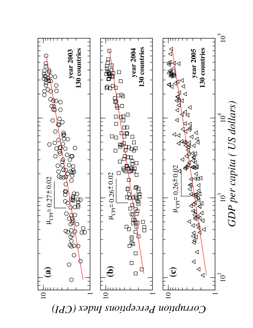
Figure 2: Log-log plots of the corruption perceptions index (CPI) versus GDP per capita (gdp) for a subset of 130 countries over the period 2003-2005. The same set of countries is presented in each plot, indicating that the power-law exponent $\mu$ characterizing the relation between CPI and gdp remains relatively stable over the considered period. As rich countries have a relatively higher gdp growth rate compared to poor countries (see Fig. 8 below), and because CPI is defined in a bounded interval, we expect the value of the exponent $\mu$ to decrease slightly with time when considering time horizons larger than a decade.

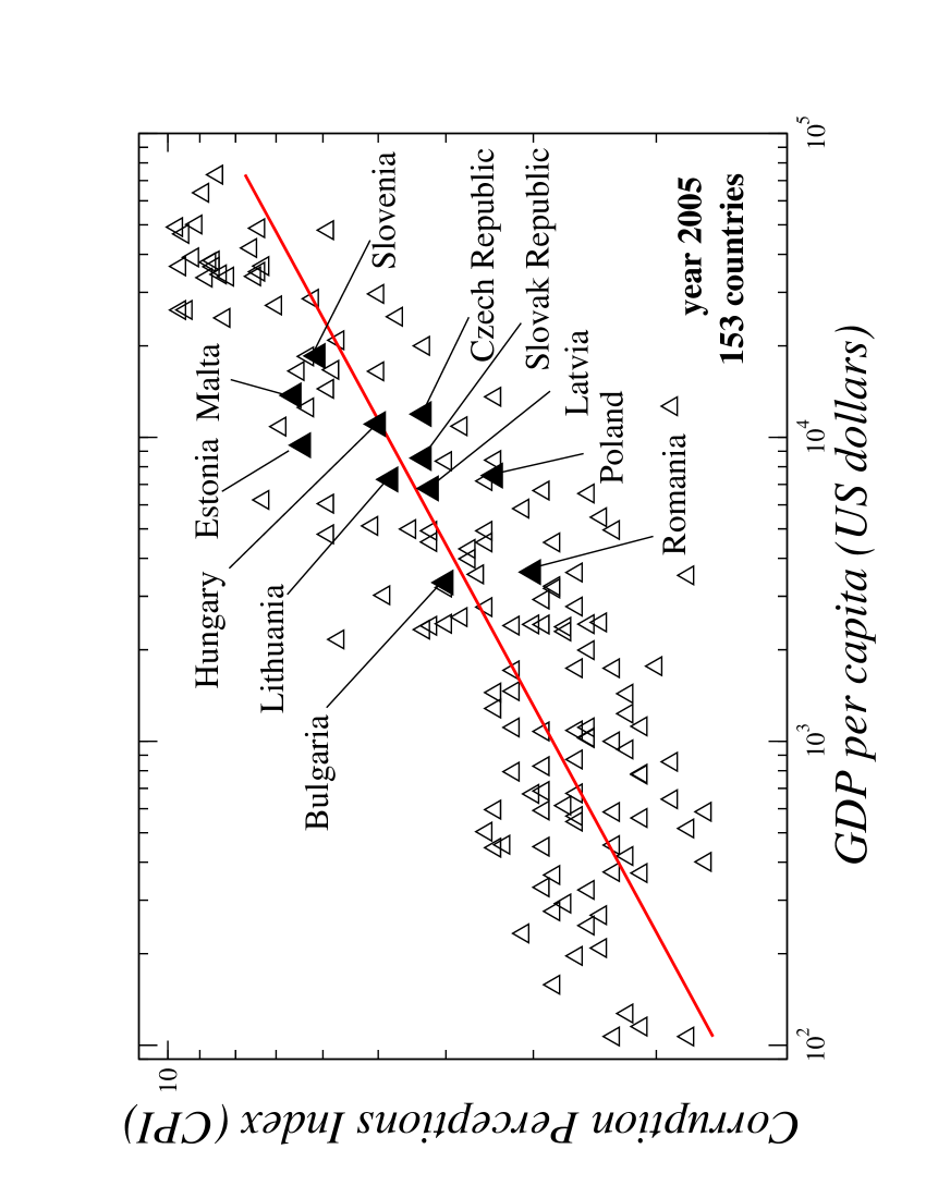
Figure 3: Same as panel (e) in Fig. 1 except we now identify by filled symbols the subset of the 153 countries, which are recently-accepted members of the European Union and candidates. Although this subset varies greatly in wealth and corruption level, data also follow a similar scale-invariant behavior.

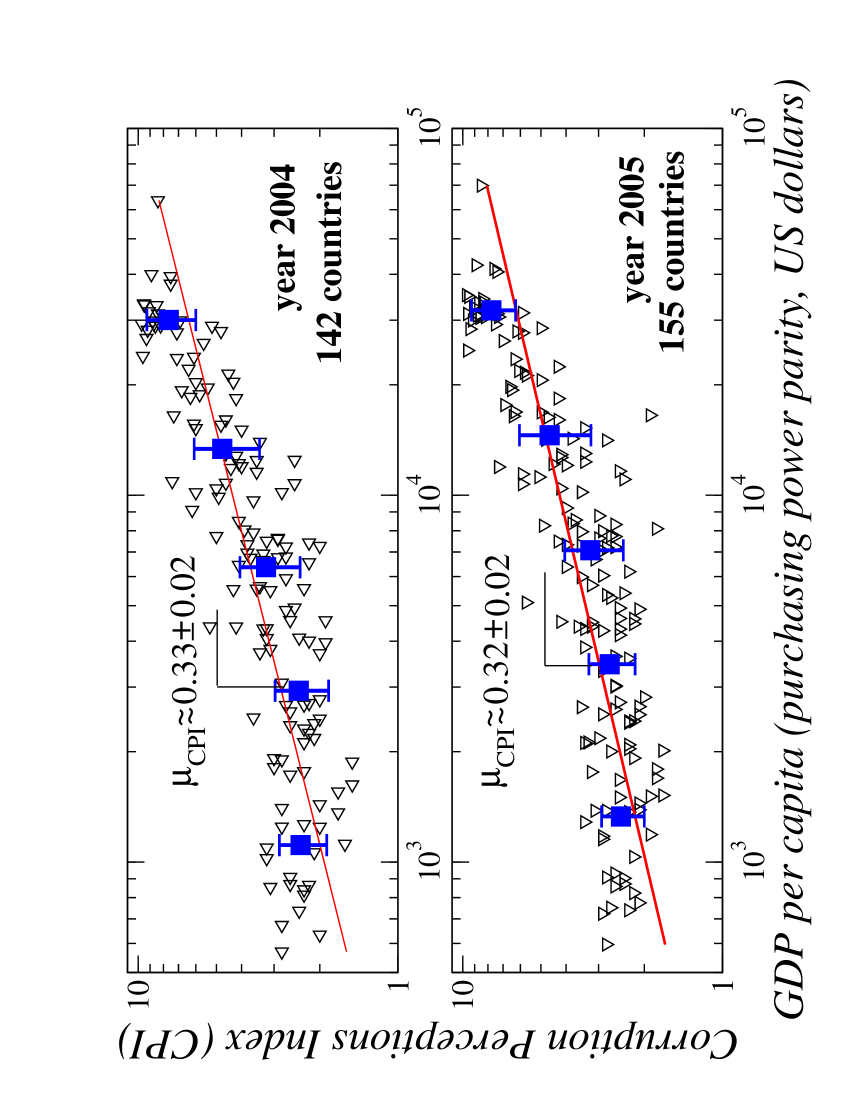
Figure 4: Log-log plots of the corruption perceptions index (CPI) versus GDP per capita (gdp) for the same years as shown in panels (d) and (e) in Fig. 1, indicating a power-law functional dependence similar to Fig. 1. Data on gdp are obtained based on purchasing power parity in U.S dollars IMFGDP . A low value of CPI corresponds to a high level of corruption CPI . The power-law relation between CPI and gdp remains stable also for constant prices across different years and different number of countries, and is characterized by a similar value of the exponent $\mu$ as for current prices. We note that the slightly higher value of $\mu_{CPI}$ observed here compared with Fig. 1 and Fig. 2 is due to the slight reduction in the different between wealthy and poor countries when gdp is measured based on purchasing power parity. The group average and standard deviation of the CPI for five subgroups of countries for both years are shown with filled squares. The power-law fit across all countries indicates the expected level of corruption for a given range of country wealth.

To confirm that our findings do not depend on the specific choice of the measure of corruption, we repeat our analysis for a different index, the CCI KKM ; CC . As the CCI is defined in the interval [–2.5, 2.5] we use a linear transformation to obtain the adjusted CCI, $CCI_{ad}~{}\equiv~{}2\times(CCI+2.5)$, so that both $CCI_{ad}$ and CPI are defined in the same interval from 0 to 10. We find that $CCI_{ad}$ also exhibits a power-law behavior as a function of gdp with a similar value of the power-law exponent $\mu$ as obtained for CPI [Fig. 1(f)]. So, the specific interval in which the corruption index is defined does not affect the nature of our findings.

We note that there is no artificially imposed scale on the values of the CPI or CCI index for different countries. While the upper and lower bounds for the CPI or CCI index are indeed pre-determined, the intrinsic relative relation between the index values for different countries is inherent to the data. There is no logarithmic scale artificially imposed on the index values of each country (see details on the CPI and CCI methodology in CPI ; CC ; method ). The fact that we obtain practically identical results (power-law dependence with similar values of the exponent $\mu$) for two independent indices CPI and CCI, which are provided by different institutions and are calculated using different methodologies, indicates that the quantitative relation of Eq. (1) is not an artifact of subjective evaluation of corruption. In summary, our empirical results indicate that the power-law relation between corruption and gdp across countries does not depend on the specific subset of chosen countries (provided they span a broad range of gdp), does not depend on the specific measure of corruption (CPI and CCI), and does not change significantly over time horizons shorter than a decade.

3.2 Corruption Level and Country Wealth Rank Curves.

We next rank countries by their gdp and by their CPI. We find that gdp versus rank exhibits an exponential behavior for countries with rank larger than 30, and a pronounced crossover to a power-law behavior for the wealthiest 30 countries [Fig. 5]. We further find that the shape of gdp versus rank curve remains unchanged for different years, and that increasing the number of countries we consider only extends the range of the exponential tail. Our findings for the shape of the gdp versus rank curve differ from earlier reports zipf1 ; zipf2 . We find that the CPI versus rank curve exhibits a behavior similarly to that of the gdp versus rank curve, with a crossover from a power law to an exponential tail for countries with rank larger than 30. The shape of the CPI versus rank curve also remains unchanged when we repeat the analysis for different years [Fig. 6]. We find that the ranking of countries based on gdp practically matches the ranking based on the CPI index. This is evidence of a strong and positive correlation between the ranking of wealth and the ranking of corruption. Since the gdp rank is an unambiguous result of an objective quantitative measure, the evidence of a strong correlation of the CPI rank with the gdp rank we observe in Fig. 5 and Fig. 6 indicates that the CPI values are not subjective, and that our finding of a power-law relation between CPI and gdp in Fig. 1 and Fig. 2 is not an artifact of an arbitrary scale imposed on the CPI or on the CCI. Further, we compare the values of the decay parameters $\zeta_{CPI}$ and $\zeta_{\it gdp}$ characterizing the exponential behavior of the CPI and gdp rank curves,

$$CPI\sim\exp(\zeta_{CPI}\cdot R_{CPI}),$$ (2)

and

$${\it gdp}\sim\exp(\zeta_{\it gdp}\cdot R_{\it gdp}),$$ (3)

where $R_{CPI}$ and $R_{\it gdp}$ index the rank order of CPI and gdp respectively.

We find that for each year the ratio $\zeta_{CPI}$/$\zeta_{\it gdp}$ reproduces the value of the power-law exponent $\mu$ defined in Eq. (1) for the same year — an insightful result since it would hold only when $R_{CPI}$ is similar to $R_{\it gdp}$. Indeed, only when $R_{CPI}\approx R_{\it gdp}$ we obtain from Eq. (2) and Eq. (3) the relation between log(CPI) and log(gdp),

$$log(CPI)\approx(\zeta_{CPI}/\zeta_{\it gdp})\cdot log({\it gdp}).$$ (4)

Combining Eq. (1) and Eq. (4), we see that

$$\mu=\zeta_{CPI}/\zeta_{\it gdp}.$$ (5)

Thus, for each year the power-law dependence between CPI and gdp in Eq. (1) is directly related to the exponential behavior of the CPI and gdp versus rank [Eq. (2) and Eq. (3)]. We note that this relation does not hold for the top 30 wealthiest countries, for which there is an enhanced economic interaction in a globalization sense, perhaps leading to similarities in development patterns and overall decrease in the gdp growth difference asloos05 ; asloos06

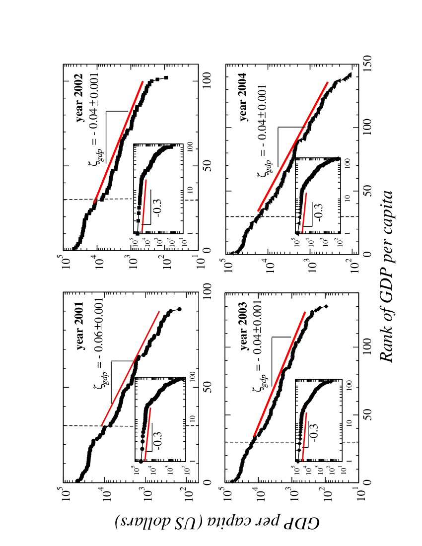
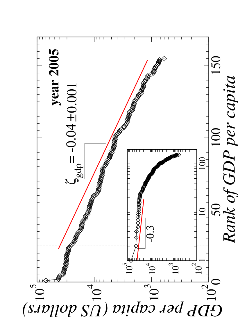
Figure 5: Zipf plots ranking in decreasing order the GDP per capita (gdp) for the same groups of countries and for the same years as shown in Fig. 1. Data on GDP per capita are obtained from the International Monetary Fund as current prices in U.S. dollars IMFGDP . Fitting lines indicate exponential behavior for the GDP per capita for countries below rank 30 (vertical dashed line, shown also in Fig. 1), characterized by the exponential decay constant $\zeta_{\it gdp}$. Log-log plots of the ranking curves (shown in the insets) indicate a crossover from an exponential to a power-law behaviour for the top 30 wealthiest countries. We note that the top 30 wealthiest countries cluster above the fitting curves in Fig. 1, Fig. 2 and Fig. 4.

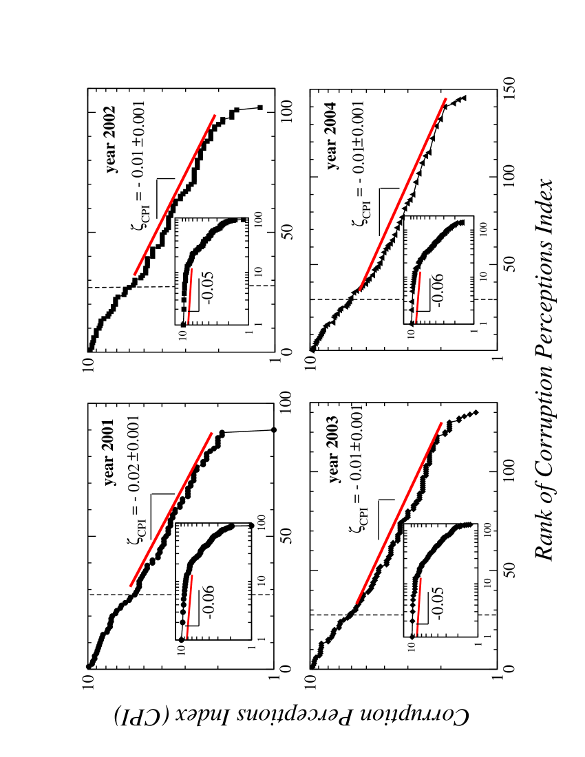
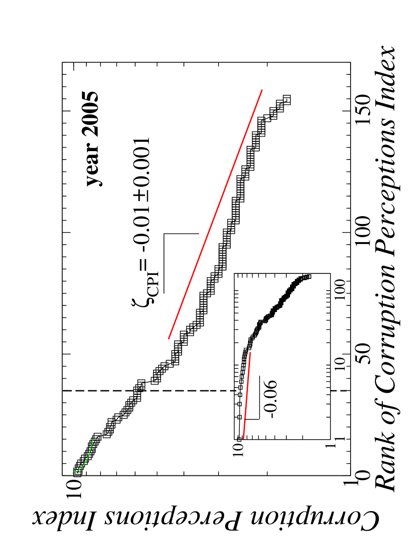
Figure 6: Zipf plots ranking in decreasing order the CPI for the same groups of countries and for the same years as shown in Fig. 1 and Fig. 5. Fitting lines indicate exponential behavior for the CPI for countries below rank 30 (vertical dashed line, shown also in Fig. 1 and Fig. 5), characterized by the exponential decay constant $\zeta_{CPI}$. The ratio $\zeta_{CPI}$/$\zeta_{\it gdp}$ consistently reproduces the value of the power-law exponent $\mu$ in Fig. 1(a) - Fig. 1(d) for each corresponding year and each group of countries. This indicates that a necessary condition for the power-law relation between CPI and GDP per capita is that the GDP per capita rank order of countries is similar to the rank order based on CPI. Log-log plots of the ranking curves (shown in the insets) indicate a crossover from an exponential to a power-law behaviour for the top 30 least corrupt countries, similar to the cross over behaviour observed for gdp in Fig. 5.

3.3 Relation Between Corruption Level and Foreign Direct Investment.

We next investigate how the corruption level relates to foreign direct investment. We consider the amount of inward investments received by different countries from the United States (U.S.). Investments originating from the U.S. are sensitive to corruption, since U.S. legislation holds American investors in other countries liable for corruption practices FCPA . We find a strong dependence of the amount of U.S. direct investments in a given country on the corruption level in that country [Fig. 7]. Specifically, we find that the functional dependence between U.S. direct investments per capita, I, and the corruption levels across countries exhibits scale-invariant behavior characterized by a power law ranging over at least a factor of $10^{3}$ [Fig. 7]

$$CPI\sim{\it I}^{\lambda}.$$ (6)

We find that less corrupt countries have received more U.S. investment per capita, and that Eq. (6) also holds for different years. In particular, we find that groups of countries from different continents, which differ in both gdp and average CPI, are characterized by different values of $\lambda$ [Fig. 7]. We obtain similar results when repeating our analysis for the CCI, suggesting that the power-law relation in Eq. (6) between corruption level and foreign direct investment per capita does not depend on the specific measure of corruption used. We also note that the 1977 Foreign Corrupt Practices Act FCPA only precludes American firms from entering corruption deals, but does not dictate in which country and how much money the American firms should invest. Therefore, the statistical regularities we find in Fig. 7 cannot arise from legislatory measures against foreign corruption.

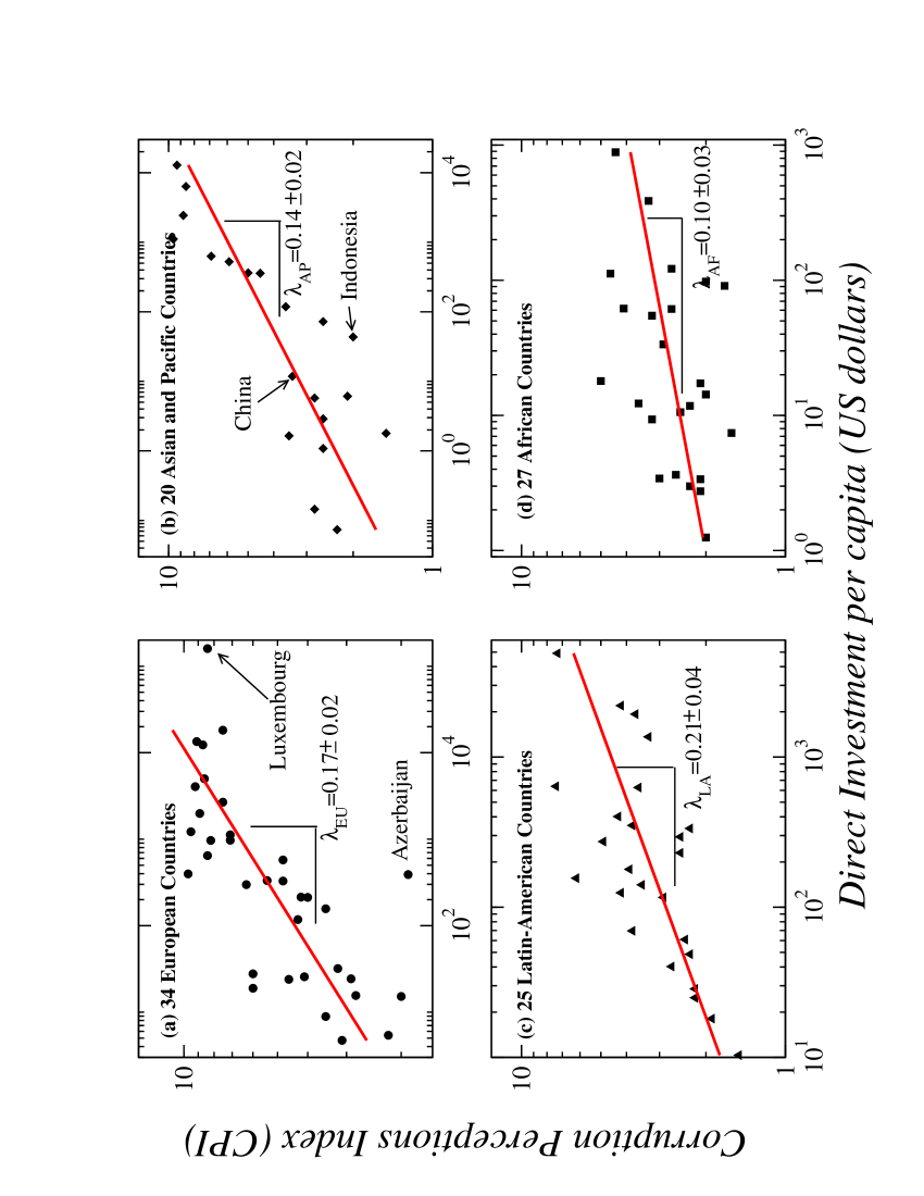
Figure 7: Log-log plots of the CPI versus the amount of direct investment on a historical-cost basis from the United States received by different countries for the year 2004 BEA . We observe strong positive correlation between level of investment per capita and level of corruption — countries with high CPI receive also larger investment. Shown are (a) 34 European countries, (b) 20 Asian-Pacific countries, (c) 25 Latin-American countries and (d) 27 African countries. Note the striking difference between the typical values of direct investment per capita when comparing, say, European countries and African countries, with typical values of $CPI\approx 5$ and $CPI\approx 2.5$ respectively. The correlation coefficients of the fits in (a), (b), (c) and (d) are 0.74, 0.83, 0.69 and 0.37 respectively. Note that although China receives a huge net inflow of U.S. investment each year, the per capita investment from the U.S. is not very high, and is quite similar to the U.S. per capita investment for countries with a CPI value similar to that of China.

3.4 Relation Between Corruption Level and Growth Rate.

Finally, we investigate whether there is a relation between corruption level and long-term growth rate. Since the CPI reflects the quality of governing and administration in a given country, which traditionally requires considerable time to change, we hypothesize that there may be relation between the current corruption level of a country and its growth rate over a wide range of time horizons. To test this hypothesis we estimate the long-term growth rate for each country as the slope of the least square fit to the plot of log(gdp) versus year over the past several decades, where the gdp is taken as constant prices in national currency [Fig. 8]. We divide all countries into four groups according to the World Bank classification based on gdp CLASS . We find a strong positive dependence between country group average of CPI and the group average long-term growth rate, showing that less corrupt countries exhibit significant economic growth while more corrupt countries display insignificant growth rates (or even display negative growth rates) [Fig. 9]. Repeating our analysis for different time horizons (1990-2005; 1980-2005) we find similar relations between the CPI and the long-term growth, indicating a link between corruption and economic growth.

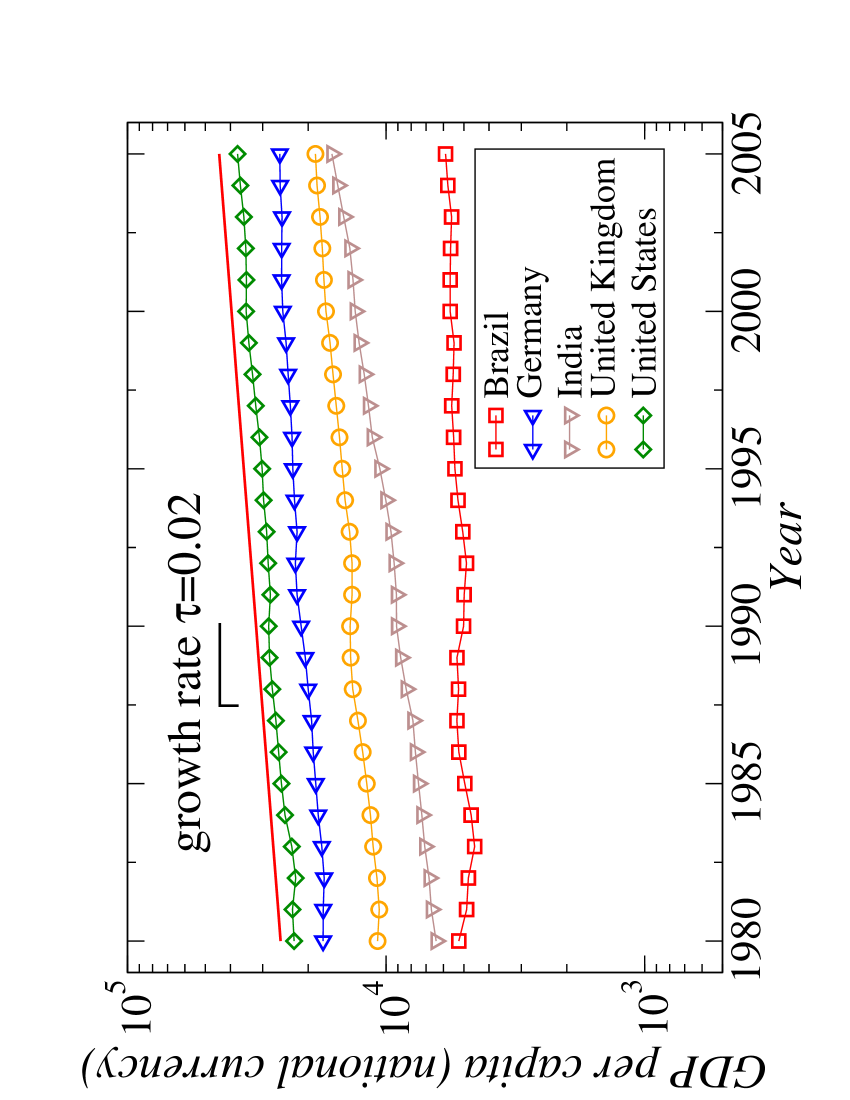
Figure 8: Long-term growth rate of the GDP per capita (gdp) measures as constant prices in national currency IMFGDP over the period 1980 to 2005. Seperate curves represent countries of different wealth and corruption level from different continents. All countries exhibit exponential growth characterized by average long-term growth rate $\tau$, estimated for each country as the slope of the least square fit to the plot of log(gdp) versus year over the period 1980 to 2005. The fitting line indicates the long-term growth rate $\tau$ of United States over the period 1980 to 2005.

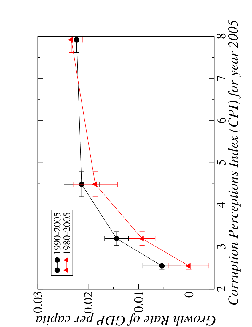
Figure 9: Relation between the CPI for the year 2005 CPI and the long-term growth rate of GDP per capita (gdp) as constant prices in national currency IMFGDP . Each curve represents 120 countries divided into 4 groups based on their level of wealth according to the World Bank’s classification CLASS . Excluded are countries with population less than two million and countries for which the GDP per capita records extend back fewer than 15 years starting from 2005. The long-term growth rate is estimated over the periods 1980-2005 and 1990-2005. Symbols represent the group average value of CPI and long-term growth rate of GDP per capita. The error bars represent the group standard error. The plot indicates that the corruption level of a country at present is strongly related to the past long-term growth rate of the GDP per capita. Countries which are presently more corrupt exhibit on average negligible or even negative growth rates. In contrast, less corrupt countries exhibit higher growth rates. This strong correlation between corruption level and growth rate of GDP per capita remains valid for a broad range of past time horizons.

In summary, the functional relations we report here can have implications when determining the relative level of corruption between countries, and for quantifying the impact of corruption when planning foreign investments and economic growth. These quantitative relations may further facilitate current studies on spread of corruption across social networks blanchard , the emergence of endogenous transitions from one level of corruption to another through cascades of agent-based micro-level interactions ross ; Situngkir , as well as when considering corruption in the context of certain cultural norms fisman .

ACKNOWLEDGMENTS: We thank F. Liljeros for valuable suggestions and discussions, and we thank D. Schmitt and F. Pammolli for helpful comments. We also thank Merck Foundation, NSF, and NIH for financial support.

References

- (1) Svensson, J. (2005) Eight Questions about Corruptions. Journal of Economic Perspectives 19: 19-42.
- (2) Mauro, P. (1995) Corruption and Growth. Quarterly Journal of Economics 110: 681-712.
- (3) Tanzi, V. Davoodi, H. R. (2000) Corruption, Growth, and Public Finance. Working Paper of the International Monetary Fund, Fiscal Affairs Department.
- (4) Leff, N. H. (1964) Economic Development Through Bureaucratic Corruption. American Behavioral Scientist 82: 337-341.
- (5) Huntington, S. P. (1968) Political Order in Changing Societies (Yale University Press, New Haven).
- (6) Wheeler, D. Mody, A. (1992) International Investment Location Decisions: The Case of U.S. Firms. Journal of International Economics 33: 57-76.
- (7) Hines, J. (1995) Forbidden Payment: Foreign Bribery and American Business After 1977. NBER Working Paper 5266.
- (8) Wei, S. J. (2000) How taxing is corruption on international investors. The Review of Economics and Statistics 82: 1-11.
- (9) Kaufmann, D. et al. (2003) Governance Matters III: Governance Indicators for 1996-2002. World Bank Policy Research Working Paper, 3106.
- (10) Knack, S. Keefer, P. (1995) Institutions and Economic Performance: Cross Country Tests Using Alternative Institutional Measures. Economics and Politics 7: 207-27.
- (11) Treisman,D. (2000) Journal of Public Economics 76: 399-457.
- (12) Jain, A. K. (2001) Corruption: A Review. Journal of Economic Surveys 15(1), 71121.
- (13) International Country Risk Guide’s corruption indicator published by Political Risk Services. Data are available at .
- (14) The Corruption Perceptions Index (CPI) is published by Transparency International. Data are available at .
- (15) The Control of Corruption Index (CCI) published by the World Bank. Data are available at .
- (16) Bardhan, P. (1997) Journal of Economic Literature 35: 1320-1346.
- (17) Lambsdorff, J. G. (1999) Corruption in Empirical Research - A Review. Transparency International Working Paper.
- (18) Schneider,F. Enste,D.H. (2000) Journal of Economic Literature 38: 77-114.
- (19) Makse, H. A. et al. (1995) Modelling Urban Growth Patterns. Nature 377: 608-612.
- (20) Axtell, R. L. (2001) Zipf Distribution of U.S. Firm Sizes. Science 293: 1818-1820.
- (21) Stanley, M. H. R. et al. (1996) Scaling Behavior in the Growth of Companies. Nature 379: 804-806.
- (22) Lee, Y. et al. (1998) Universal Features in the Growth Dynamics of Complex Organizations. Phys. Rev. Lett. 81: 3275-3278.
- (23) Fu, D. et al. (2005) The Growth of Business Firms: Theoretical Framework and Empirical Evidence. Proc. Natl. Acad. Sci. 102: 18801-18806.
- (24) Plerou, V. et al. (1999) Similarities between the Growth Dynamics of University Research and of Competitive Economic Activities. Nature 400: 433-437.
- (25) Ivanov, P. Ch. et al. (2004) Common scaling patterns in intertrade times of US stocks. Physical Review E 69(5): 056107.
- (26) Newman M. E. J., (2005) Power laws, Pareto distributions and Zipfs law. Contemporary Physics 46: 323-351.
- (27) For details on the methodology in computing the CPI see ”The Methodology of the 2005 Corruption Perceptions Index”, available at: .
-
(28)
GDP per capita data as current prices in U.S. dollars and as constant prices in national currency
are provided by the International Monetary Fund, WORLD ECONOMIC OUTLOOK Database,
September 2005.
. -
(29)
U.S. Direct Investment Position data are obtained from
. - (30) Information regarding the Foreign Corrupt Practices Act (FCPA) of 1977 is available at .
- (31) Di Guilmi, C. et al. (2003) Power Law Scaling in the World Income Distribution. Economics Bulletin 15: 1-7.
- (32) Iwahashi, R. Machikita, T. (2004) A new empirical regularity in world income distribution dynamics, 1960-2001. Economics Bulletin 6: 1-15.
- (33) Miskiewicz J, Ausloos M. Correlations between the most developed (G7) countries. A moving average window size optimisation. (2005) Acta Physica Polonica B 36 (8): 2477-2486.
- (34) Miskiewicz J, Ausloos M. An attempt to observe economy globalization: The cross correlation distance evolution of the top 19 GDP’s. (2006) International Journal of Modern Physics C 17 (3): 317-331.
- (35) Information regarding the classification of countries based on their gross domestic product per capita is provided by the World Bank, at: .
- (36) Blanchard, Ph. et al. (2005) The Epidemics of Corruption. arxiv.org/abs/physics/0505031.
- (37) Hammond, R. (2000) Endogenous Transition Dynamics in Corruption: An Agent-Based Computer Model. CSED Working Paper No. 19.
- (38) Situngkir, H. (2004) Money-Scape: A Generic Agent-Based Model of Corruption. Computational Economics.
- (39) Fisman, R. Miguel, E. (2006) Cultures of Corruption: Evidence from Diplomatic Parking Tickets. NBER working paper No. 12312.