Probing dark energy with cluster counts and cosmic shear power spectra: including the full covariance

Abstract

Several dark energy experiments are available from a single large-area imaging survey, and may be combined to improve cosmological parameter constraints and/or test inherent systematics. Two promising experiments are cosmic shear power spectra and counts of galaxy clusters. However the two experiments probe the same cosmic mass density field in large-scale structure, therefore the combination may be less powerful than first thought.

We investigate the cross-covariance between the cosmic shear power spectra and the cluster counts based on the halo model approach, where the cross-covariance arises from the three-point correlations of the underlying mass density field. Fully taking into account the cross-covariance as well as non-Gaussian errors on the lensing power spectrum covariance, we find a significant cross-correlation between the lensing power spectrum signals at multipoles $l\sim 10^{3}$ and the cluster counts containing halos with masses $M\lower 2.15277pt\hbox{$\;\buildrel>\over{\sim}\;$}10^{14}M_{\odot}$. Including the cross-covariance for the combined measurement degrades and in some cases improves the total signal-to-noise ratios up to $\sim\pm 20\%$ relative to when the two are independent. For cosmological parameter determination, the cross-covariance has a smaller effect as a result of working in a multi-dimensional parameter space, implying that the two observables can be considered independent to a good approximation. We also discuss that cluster count experiments using lensing-selected mass peaks could be more complementary to cosmic shear tomography than mass-selected cluster counts of the corresponding mass threshold. Using lensing selected clusters with a realistic usable detection threshold ($(S/N)_{\rm cluster}\sim 6$ for a ground-based survey), the uncertainty on each dark energy parameter may be roughly halved by the combined experiments, relative to using the power spectra alone.

I Introduction

In recent years great observational progress has been made in measuring the constituents of the universe (e.g. spergelea06 ; coleetal05 ; tegmarketal06 ). It appears that the universe is currently dominated by an unexpected component that is causing the universe to accelerate in its expansion. This component is dubbed “dark energy”. Understanding the nature of dark energy is one of most fundamental questions that remain unresolved with the current cosmological data sets (e.g. weinberg89 ; ratrapeebles88 ). This is now the focus of several planned future surveys panstarrs ; DES ; HSC ; LSST ; WFMOS ; DUNE ; SNAP .

Whether the accelerating expansion is as a consequence of the cosmological constant, a new fluid or a modification to Einstein’s gravity, these future surveys will provide key information. In addition they will provide a wealth of further cosmological information, such as constraints on the neutrino mass and the spectrum of primordial perturbations generated in the early universe (e.g. TKF06 ).

Combining several techniques accessible from different cosmological observables is often a powerful way to improve constraints on cosmology. However, care must be taken if the observables are not completely independent. Two of the most promising methods for constraining the dark energy are galaxy cluster counts and cosmic shear (e.g. DETF ).

Clusters of galaxies contain galaxies, hot gas and dark matter in ratio approximately 1:10:100 Sarazin88 . They are the largest gravitationally bound objects in the universe and the number of clusters of galaxies has long been recognized as a powerful probe of cosmology lilje92 ; bahcallc93 ; hanami93 ; whiteef93 ; KitayamaSuto97 . Counting clusters of galaxies as a function of redshift allows a combination of structure growth and geometrical information to be extracted, thus potentially allowing constraints on the nature of dark energy Haimanetal00 ; Welleretal02 ; LimaHu04 ; Wangetal04 ; MarianBernstein06 . If cluster masses can be measured accurately then the shape of the mass function also helps to break degeneracies Hu03 . The distribution of clusters on the sky (e.g. two-point correlation function) carries additional information on dark energy MajumdarMohr04 ; HuHaiman03 .

The bending of light by mass, gravitational lensing, causes images of distant galaxies to be distorted. These sheared source galaxies are mostly too weakly distorted for us to measure the effect in single galaxies, but require surveys containing a few million galaxies to detect the signal in a statistical way. This cosmic shear signal has been observed vanwaerbekeea00 ; baconre00 ; wittmanea00 ; kaiseretal00 and used to constrain cosmology (most recently jarvisetal05 ; hoekstraea06 ; masseyea07 ; Schimdetal07 ). By using redshift information of source galaxies the evolution of the dark matter distribution with redshift can be inferred. Hence, measuring the cosmic shear two-point function as a function of redshift and separation between pairs of galaxies can be used to constrain the geometry of the universe as well as the growth of mass clustering. This method has emerged as one of the most promising to obtain precise constraints on the nature of dark energy if systematics are well under control Hu99 ; Huterer02 ; TJ04 .

Future optical imaging surveys suitable for cosmic shear analysis will also allow the identification of clusters of galaxies. This could be done either using the colors of the cluster members (e.g. koesterea07 ; gladdersy05 ) or using peaks in the gravitational lensing shear field (e.g. Miyazakietal02 ; Wittmanetal06 ; Miyazakietal07 ). In addition cluster surveys in other wavebands will overlap with the cosmic shear surveys allowing detection using X-rays and the thermal Sunyaev–Zel’dovich (SZ) effect.

Clusters of galaxies produce a large gravitational lensing effect on distant galaxies, therefore cluster counts and cosmic shear will not be strictly statistically independent. The volume surveyed is finite and therefore the number of clusters observed will not be exactly equal to the average over all universe realizations. If the number of clusters happens to be higher for a given survey region, then the cosmic shear signal is also likely to be higher. Although the volumes will be large, and thus the deviation is small, this may amount to a significant uncertainty in the dark energy parameters as obtained by cluster counts, and dominates the non-Gaussian errors on the cosmic shear HuWhite01 ; coorayhu01 ; KilbingerSchneider05 ; TJ07 .

One aspect of this cross-correlation was discussed in FangHaiman06 and found to be negligible. However, here we make a full treatment of this effect using the halo model for non-linear structure formation, and quantify the resulting change in joint constraints on the dark energy parameters.

The structure of our paper is as follows. In § II we describe how our observables, cluster number counts and lensing power spectra, can be expressed in terms of the background cosmological model and the density perturbations. In § III, we describe a methodology to compute covariances of the cluster counts and the lensing power spectra, and the cross-covariance between the two observables. The detailed derivations of the covariances are presented in Appendix. In § IV we first study the total signal-to-noise ratios expected for a joint experiment of the cluster counts and the lensing power spectrum fully including the cross-covariance predicted from the $\Lambda$CDM cosmologies. We then present forecasts for cosmological parameter determination for the joint experiment, with particular focus on forecasts for the dark energy parameter constraints. Finally, we present conclusions and discussion in § V.

II Preliminaries

II.1 A CDM model

We work in the context of spatially flat cold dark matter models for structure formation. The expansion history of the universe is given by the scale factor $a(t)$ in a homogeneous and isotropic universe (e.g., see Dodelson ). We describe the Universe in terms of the matter density $\Omega_{\rm m}$ (the cold dark matter plus the baryons) and dark energy density $\Omega_{\rm de}$ at present (in units of the critical density $3H_{0}^{2}/(8\pi G)$, where $H_{0}=100~{}h~{}{\rm km}~{}{\rm s}^{-1}~{}{\rm Mpc}^{-1}$ is the Hubble parameter at present). In general the expansion rate, the Hubble parameter, is given by

$$H^{2}(a)=H_{0}^{2}\left[\Omega_{\rm m}a^{-3}+\Omega_{\rm de}e^{-3\int^{a}_{1}da^{\prime}(1+w(a^{\prime}))/a^{\prime}}\right],$$ (1)

where we have employed the normalization $a(t_{0})=1$ today and $w(a)$ specifies the equation of state for dark energy as $w(a)\equiv p_{\rm de}(a)/\rho_{\rm de}(a)$. Note that $\Omega_{\rm m}+\Omega_{\rm de}=1$ and $w=-1$ corresponds to a cosmological constant. The comoving distance $\chi(a)$ from an observer at $a=1$ to a source at $a$ is expressed in terms of the Hubble parameter as

$$\chi(a)=\int^{1}_{a}\!\!\frac{da^{\prime}}{H(a^{\prime})a^{\prime 2}}.$$ (2)

This gives the distance-redshift relation $\chi(z)$ via the relation $1+z=1/a$.

Next we need the redshift growth of density perturbations. In linear theory after matter-radiation equality, all Fourier modes of the mass density perturbation, $\delta(\mbox{\boldmath$x$})(\equiv\delta\rho_{m}(\mbox{\boldmath$x$})/\bar{\rho}_{m})$, grow at the same rate, the growth rate (e.g. see Eq. 10 in Takada06 for details).

II.2 Number counts of galaxy clusters

The galaxy cluster observables we will consider in this paper are the number counts drawn from a given survey region. Clusters can be found via their notable observational properties such as gravitational lensing, member galaxies, X-ray emission and the SZ effect. For number counts we simply treat clusters as points; in other words, we do not care about the distribution of mass within a cluster. Hence, the number density field of clusters at redshift $z$ can be expressed as

$$n_{\rm cl}(\mbox{\boldmath$x$})=\sum_{i}S(m_{i};z)\delta_{D}^{3}(\bm{x}-\bm{x}_{i}),$$ (3)

where $\delta_{D}^{3}(\mbox{\boldmath$x$})$ is the three-dimensional Dirac delta function. The summation runs over halos (the subscript $i$ stands for the $i$-th halo), and $S(m_{i};z)$ denotes the selection function that discriminates the halos used for the cluster number counts statistic from other halos.

In this paper, we will consider the following two toy models for the selection function, to develop intuition for the importance of cross-correlation between cluster counts and the lensing power spectrum and to make a comparison between cosmological parameter estimations derived from different cluster samples. Note that throughout this paper we will ignore uncertainties associated with cluster mass-observable relation, which could significantly degrade the ability of cluster counts for constraining cosmological parameters (e.g. LimaHu04 ). We shall discuss this issue in § IV.5.

A mass-limited cluster sample – The first toy model we will consider is a mass-limited cluster sample. For this model, we include all halos with masses above a given mass threshold:

$$S(m;z)=\left\{\begin{array}[]{ll}1,&\mbox{if $m\geq M_{\rm min}$}\\ 0,&\mbox{otherwise}.\end{array}\right.$$ (5)

To a zero-th order approximation, the mass-limited selection may mimic a cluster sample derived from a flux-limited survey of clusters via the SZ effect, as this effect is free of the surface brightness dimming effect (e.g. see (CarlstromHolderReese02, )).

A lensing-based cluster sample – A lensing measurement allows one to make a reconstruction of the two-dimensional mass distribution projected along the line of sight KaiserSquires93 . A high peak in the mass map provides a strong candidate for a massive cluster (see Miyazakietal02 ; Wittmanetal06 ; Miyazakietal07 for an implementation of this method to actual data). To be more explicit, one can define height or significance for each peak in the reconstructed mass map using the effective signal-to-noise ratio (see HTY for details):

$$\left(\frac{S}{N}\right)_{\rm cluster}\equiv\frac{\kappa_{\rm cluster}(m,z)}{\sigma_{\rm N}}.$$ (6)

Here $\kappa_{\rm cluster}$ is the convergence amplitude due to a given cluster at redshift $z$ and with mass $m$, and $\sigma_{\rm N}$ is the rms fluctuations in $\kappa$ due to the intrinsic ellipticity noise arising from a finite number of the background galaxies. Note that we assume an NFW profile NFW with profile parameters modeled in TJ03a , and consider the convergence field smoothed with a Gaussian filter of angular scale $\theta_{s}=1^{\prime}$. To compute the $(S/N)_{\rm cluster}$ for a cluster at redshift $z$, we take into account the remaining fraction of background galaxies behind the cluster for a given redshift distribution of whole galaxy population (see § IV.1). This accounts for the variation of mean redshift and number density of the background galaxies with cluster redshift, which changes both the signal and the intrinsic noise in Eq. (6).

From the reconstructed mass map, a cluster sample may be constructed by counting mass peaks with heights above a given threshold, $\nu_{\rm min}$: the selection function is given by

$$S(m;z)=\left\{\begin{array}[]{ll}1,&\mbox{if $(S/N)_{\rm cluster}\geq\nu_{\rm min}$}\\ 0,&\mbox{otherwise}.\end{array}\right.$$ (8)

As carefully investigated in HTY , the minimum mass of clusters detectable with a given threshold varies with cluster redshift; clusters at medium redshift between observer and a typical source redshift are most easily detectable, while only more massive clusters can be detected at redshifts smaller and greater than the medium redshift, as discussed below.

We will employ the halo model to quantify the statistical properties of cluster observables. In the halo model approach, we assume that all the matter is in halos. Following the formulation developed in ScherrerBertschinger91 ; Scoccimarroetal01 ; TJ03a ; TJ03b (also see Appendix A.1 and CooraySheth for a thorough review), the ensemble average of Eq. (3) can be computed as

$$\bar{n}_{\rm cl} \equiv \left\langle{n_{\rm cl}(\mbox{\boldmath$x$})}\right\rangle=\left\langle{\sum_{i}S(m_{i};z)\delta_{D}^{3}(\bm{x}-\bm{x}_{i})}\right\rangle$$ (9)

$$= \left\langle{\int\!\!dm~{}\int\!\!d\bm{x}^{\prime}\sum_{i}S(m;z)\delta_{D}^{3}(\bm{x}-\bm{x}^{\prime})}\right.$$

$$\times\left.{\delta_{D}(m-m_{i})\delta_{D}^{3}(\bm{x}^{\prime}-\bm{x}_{i})}\right\rangle$$

$$= \int\!\!dm~{}S(m;z)n(m)\int\!\!d\bm{x}^{\prime}\delta_{D}^{3}(\bm{x}-\bm{x}^{\prime})$$

$$= \int\!\!dm~{}S(m;z)n(m),$$

where $n(m)$ is the halo mass function corresponding to the redshift considered and we have used the ensemble average $\langle{\sum_{i}\delta_{D}(m-m_{i})\delta_{D}^{3}(\bm{x}_{i}-\bm{x}^{\prime})}\rangle=n(m)$. Thus, as expected, the ensemble average of the cluster number density field is given by the integral of the halo mass function, which does not depend on the cluster distribution and spatial position. For the halo mass function, we employ the Sheth-Tormen fitting formula ShethTormen , modified from the original Press-Schechter function PressSchechter . Note that we use parameter values $a=0.75$ and $p=0.3$ in the formula following the discussion in HuKravtsov03 . We assume that the mass function can be applied to dark energy cosmologies by replacing the growth rate appearing in the formula with that for a dark energy model LinderJenkins .

A more useful quantity often considered in the literature is the total number counts of clusters available from a given survey, which is obtained by integrating the three-dimensional number density field over a range of redshifts surveyed. Cluster redshifts are rather easily available even from a multicolor imaging survey alone because their central bright galaxies, or red sequence galaxies, have secure photometric redshift estimates. Having these facts in mind we will use as our observable the angular number density averaged over a survey area and divided into redshift bins:

$${\cal N}_{(b)\rm cl} = \int\!\!d^{2}\bm{\theta}~{}W(\bm{\theta})\int_{0}^{\chi_{H}}\!\!d\chi~{}\frac{d^{2}V}{d\chi d\Omega}$$ (10)

$$\times\sum_{i}S_{(b)}(m_{i};z)\delta_{D}(\chi-\chi_{i})\delta_{D}^{2}(\chi\bm{\theta}-\chi_{i}\bm{\theta}_{i}),$$

where $W(\bm{\theta})$ is the window function of the survey defined so that it is normalized as $\int\!\!d^{2}\bm{\theta}W(\bm{\theta})=1$, $\chi_{H}$ is the distance to the Hubble horizon, and the comoving volume per unit comoving distance and unit steradian is given by $d^{2}V/d\chi d\Omega=\chi^{2}$ for a flat universe. The subscript in the round bracket, $(b)$, stands for the $b$-th redshift bin for the cluster number counts. In the following, we will simply consider the sharp redshift selection function

$$S_{(b)}(m_{i};z)\rightarrow\left\{\begin{array}[]{ll}S(m_{i}),&\mbox{if $z_{(b),{\rm lower}}\leq z\leq z_{(b),{\rm upper}}$}\\ 0,&\mbox{otherwise.}\end{array}\right.$$ (13)

Note that the redshift $z$ appearing in the argument of $S_{(b)}(m_{i};z)$ is related to the comoving distance $\chi$ via the relation $d\chi=dz/H(z)$.

Using the halo model, the expectation value of the angular number density can be computed from the ensemble average of Eq. (10) as

$$N_{(b)} \equiv \langle{{\cal N}_{(b)}}\rangle$$ (14)

$$= \int\!\!d^{2}\bm{\theta}W(\bm{\theta})\!\int^{\chi_{H}}_{0}\!\!d\chi\frac{d^{2}V}{d\chi d\Omega}\int\!\!dm~{}S_{(b)}(m;z)n(m)$$

$$= \int^{\chi_{H}}_{0}\!\!d\chi~{}\frac{d^{2}V}{d\chi d\Omega}\int\!\!dm~{}S_{(b)}(m;z)n(m).$$

Thus, the expectation value again does not depend on the cluster distribution. The sensitivity of the number density to dark energy arises from the comoving volume and the mass function $n(m)$ Haimanetal00 .

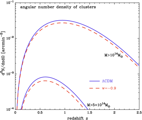
Figure 1: The average angular number density of halos with masses above a given threshold, per unit square arcminute and per unit redshift interval. The upper pair and lower pair of curves are for halos with $M/M_{\odot}\geq 10^{14}$ and $5\times 10^{14}$, respectively. Increasing the dark energy equation state from $w=-1$ to $w=-0.9$ decreases the number density, as shown by the dashed curves.

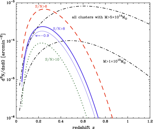
Figure 2: As in the previous plot, but shown here is the number density for the lensing-based cluster sample, where clusters having a lensing signal greater than a given detection threshold are selected in the sample as described around Eq. (8). The dashed, solid and dotted curves show the results for the detection thresholds $(S/N)_{\rm cluster}\geq 6,8$ and $10$, respectively. For comparison, the two dot-dashed curves show the number density for the mass-selected cluster sample with masses $M/M_{\odot}\geq 5,10\times 10^{14}$. Increasing $w_{0}$ from $w_{0}=-1.0$ to $w_{0}=-0.9$ leads to a decrease in the number density as shown by the thin-solid curve, compared to the bold-solid curve. The lensing selected number densities peak at a redshift $z\sim 0.25$, reflecting redshift dependence of the lensing efficiency function for source galaxies at $z_{\rm s}\sim 1$.

Fig. 1 shows the average angular number density of halos with masses greater than a given threshold, per unit square arcminute and per unit redshift interval assuming the fiducial model defined in IV.1. Increasing the dark energy equation of state from our fiducial model $w=-1.0$ to $w=-0.9$ decreases the number density, because the change decreases both the comoving volume $d^{2}V/d\chi d\Omega$ and the number density of cluster-scale halos, for a given CMB normalization of density perturbations. Comparing the results for mass thresholds $M_{\rm min}/M_{\odot}=10^{14}$ and $5\times 10^{14}$ clarifies that a factor 5 increase in the mass threshold leads to a significant decrease in the number density, reflecting the mass sensitivity of the halo mass function in its exponential tail.

In Fig. 2 we present the number density for the lensing-based cluster sample in which clusters having a lensing signal greater than a given detection threshold are included in the sample as discussed around Eq. (8). Note that to compute the results shown in this plot we assumed the redshift distribution of galaxies described in § IV.1 and the NFW mass profile to model the cluster lensing. In practice high detection thresholds such as $(S/N)_{\rm cluster}\lower 2.15277pt\hbox{$\;\buildrel>\over{\sim}\;$}6$ are necessary in order to make robust estimates for cluster counts, because contamination of false peaks due to intrinsic ellipticities or the projection effect are expected to be low for such high thresholds (see WhiteVanWaerbeke02 ; HTY for the details). Comparing with the number density for a mass-selected sample shown by the dot-dashed curves, one can roughly find which mass and redshift ranges of clusters are probed by the lensing-based cluster sample. For example, the cluster sample with lensing signal $(S/N)_{\rm cluster}\geq 10$ contains massive clusters with masses $M\lower 2.15277pt\hbox{$\;\buildrel>\over{\sim}\;$}10^{15}M_{\odot}$ over redshift ranges $z\lower 2.15277pt\hbox{$\;\buildrel<\over{\sim}\;$}0.4$, while only even more massive clusters are included in the sample at the higher redshifts. This cluster sample has a narrower redshift coverage than the simple mass threshold; all the curves peak at a redshift $z\sim 0.25$. The peak redshift is mainly attributed to redshift dependence of the lensing efficiency for source galaxies of $z_{s}\sim 1$ in our redshift distribution. A change of $w_{0}$ from $w_{0}=-1.0$ to $w_{0}=-0.9$ leads to a decrease in the number density, as seen in Fig. 1. As before the effect comes partially arises from the decrease in comoving volume and the change in the halo mass function. Unlike the simple mass threshold case, there is now an additional contribution to the decrease in number density caused by the lower lensing efficiency and thus lower $S/N$ for a cluster of a given mass and redshift.

II.3 Lensing power spectrum with tomography

Gravitational shear can be simply related to the lensing convergence: the weighted mass distribution integrated along the line of sight. Photometric redshift information on source galaxies allows us to subdivide galaxies into redshift bins (we will discuss possible effects of photometric redshift errors on our results in § IV.5). This allows more cosmological information to be extracted, which is referred to as lensing tomography (e.g., see Mellier99 ; BartelmannSchneider ; Schneider06 for a thorough review, and see Hu99 ; Huterer02 ; TJ04 for the details of lensing tomography).

In the context of cosmological gravitational lensing the convergence field with tomographic information is expressed as a weighted projection of the three-dimensional mass density fluctuation field:

$$\kappa_{(i)}(\mbox{\boldmath$\theta$})=\int_{0}^{\chi_{H}}\!\!d\chi W_{(i)g}(\chi)\delta[\chi,\chi\mbox{\boldmath$\theta$}],$$ (15)

where $\theta$ is the angular position on the sky, and $W_{(i)g}$ is the gravitational lensing weight function for source galaxies sitting in the $i$-th redshift bin (see Eq. (10) in TJ04 for the definition). Note that, hereafter, quantities with subscripts in the round bracket such as $(i)$ stands for those for the $i$-th redshift bin. To avoid confusion, throughout this paper we use $i,j$ or $i^{\prime},j^{\prime}$ for the lensing power spectrum redshift bins, and $b,b^{\prime}$ for the cluster count redshift bins.

The lensing tomographic information allows us to extract redshift evolution of the lensing weight function as well as the growth rate of mass clustering. These are both sensitive to dark energy. For example, increasing the equation of state parameter $w$ from $w=-1$ lowers $W_{(i)g}$ as well as suppressing the growth rate at lower redshifts. Therefore when the CMB normalization of density perturbations is employed, an increase in $w$ decreases the lensing power spectrum due to both the lower $W_{(i)g}$ and the lower matter power spectrum amplitude. The sensitivity of lensing observables to the dark energy equation of state roughly arises equally from the two effects (e.g., see simpsonb05 ).

The cosmic shear fields are measurable only in a statistical way. The most conventional methods used in the literature are the shear two-point correlation function. The Fourier transformed counterpart is the shear power spectrum. The convergence power spectrum is identical to the shear power spectrum but is easier to work with as it is a scalar. Using the flat-sky approximation Limber , the angular power spectrum between the convergence fields of redshift bins $i$ and $j$ is found to be

$$P_{(ij)\kappa}(l)=\int_{0}^{\chi_{H}}\!\!d\chi W_{(i)g}(\chi)W_{(j)g}(\chi)\chi^{-2}P_{\delta}\!\left(k=\frac{l}{\chi};\chi\right),$$ (16)

where $P_{\delta}(k)$ is the three-dimensional mass power spectrum. We can safely employ the flat-sky approximation for our purpose, because a most accurate measurement for the lensing power spectrum is available around multipoles $l\sim 1000$ for a ground-based survey of our interest (e.g. see Fig. 1 in Jainetal07 ), and the flat-sky approximation serves as a very good approximation on these small scales Hu00 .

For $l\lower 2.15277pt\hbox{$\;\buildrel>\over{\sim}\;$}100$ the major contribution to $P_{(ij)\kappa}(l)$ comes from non-linear clustering (e.g., see Fig. 2 in TJ04 ). We employ the fitting formula for the non-linear $P_{\delta}(k)$ proposed in Smith et al. Smith , assuming that it can be applied to dark energy cosmologies by replacing the growth rate used in the formula with that for a given dark energy model. We note in passing that the issue of accurate power spectra for general dark energy cosmologies still needs to be addressed carefully (see HutererTakada ; Ma07 for related discussion).

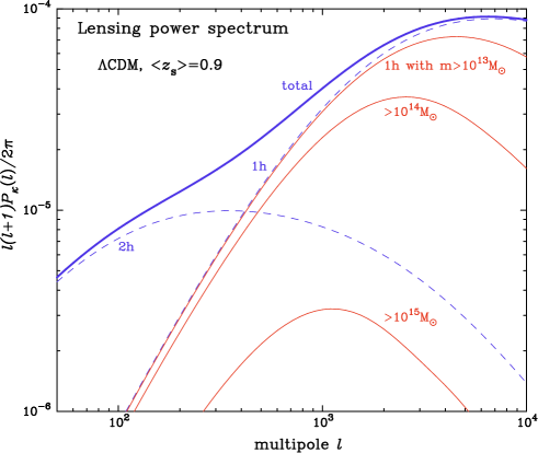
Figure 3: A lensing power spectrum for the non-tomographic case (i.e. one redshift bin) for a $\Lambda$CDM model, expected for a ground-based survey that probes galaxies with mean redshift $\langle{z_{s}}\rangle=0.9$. The two thin dashed curves show the 1- and 2-halo term contributions to the power spectrum, while the bold curve shows the total power. The three thin solid curves show the 1-halo term contributions obtained when the lensing effects on background galaxies due to halos with masses $M/M_{\odot}\geq 10^{15},10^{14},10^{13}$ are included, respectively.

Fig. 3 demonstrates how lensing of background galaxies by clusters contributes to the lensing power spectrum. Note here that we have employed the halo model developed in Takada & Jain TJ03a ; TJ03b to compute the mass power spectrum, although we will use the Smith et al. fitting formula to compute the lensing power spectrum in most parts of this paper instead. Briefly, to compute the spectra based on the halo model approach, we need to model three ingredients: (i) the halo mass function (see also the description below Eq. [9]); (ii) the profile for the mass distribution around a halo; and (iii) the halo bias parameter.

It is clear that the convergence on scales $l\lower 2.15277pt\hbox{$\;\buildrel>\over{\sim}\;$}100$ is significantly boosted by the existence of non-linear structures, halos. In this paper we are especially interested in using the lensing information inherent in angular scales $l\lower 2.15277pt\hbox{$\;\buildrel<\over{\sim}\;$}3000$ to constrain dark energy, and a fair fraction of the power at scales $l\sim 10^{3}$, up to $\sim 60\%$ of the total power, arises from massive halos with $M\lower 2.15277pt\hbox{$\;\buildrel>\over{\sim}\;$}10^{14}M_{\odot}$. The 1-halo term contribution is given by redshift-space integral of the halo mass function and halo profiles weighted with the lensing efficiency. The results imply that, if massive clusters with $M\lower 2.15277pt\hbox{$\;\buildrel>\over{\sim}\;$}10^{14}M_{\odot}$ happen to be less or more populated in a survey region, amplitudes of the observed lensing power spectrum from the survey are very likely to be smaller or greater than expected, respectively. Therefore, a cross-correlation between the lensing power spectrum and the cluster counts are intuitively expected, if both of the observables are measured from the same survey region.

In reality, the observed power spectrum is contaminated by the intrinsic ellipticity noise. Assuming that the intrinsic ellipticity distribution is uncorrelated between different galaxies, the observed power spectrum between redshift bins $i$ and $j$ can be expressed as

$$P^{\rm obs}_{(ij)\kappa}(l)=P_{(ij)\kappa}(l)+\delta^{K}_{ij}\frac{\sigma_{\epsilon}^{2}}{\bar{n}_{(i)}}$$ (17)

where $\sigma_{\epsilon}$ is the rms of intrinsic ellipticities per component, and $\bar{n}_{(i)}$ denotes the average number density of galaxies in the $i$-th redshift bin. The Kronecker delta function, $\delta^{K}_{ij}$, accounts for the fact that the cross-spectra of different redshift bins ($i\neq j$) are not affected by the shot noise contamination. We will omit the superscript ‘obs’ when referring to $P_{\kappa}^{\rm obs}(l)$ in the following for notational simplicity.

III Covariances of lensing power spectrum and cluster observables

To estimate a realistic forecast for cosmological parameter constraints for a given survey we have to quantify sources of statistical error on observables of interest, the cluster number counts and the lensing power spectrum, and then propagate the errors into the parameter forecasts. In this section, we will present the covariance matrices of the observables.

III.1 Covariances of the cluster number counts

The cluster observables can be naturally incorporated in the halo model approach, allowing us to compute the statistical properties in a straightforward way. In this paper we focus on the average angular number density of clusters drawn from a survey, also subdivided into redshift bins as described in § II.2. The covariance between the average number densities in redshift bins $b$ and $b^{\prime}$, given by Eq. (10), is defined as

$$[\bm{C}]^{c}_{bb^{\prime}} \equiv \langle{{\cal N}_{(b)}{\cal N}_{(b^{\prime})}}\rangle-N_{(b)}N_{(b^{\prime})}.$$ (18)

Based on the halo model the covariances of the angular number density can be derived in Appendix B.1 (also see HuKravtsov03 for the original derivation) as

$$[\bm{C}^{c}]_{bb^{\prime}} = \delta^{K}_{bb^{\prime}}\frac{N_{(b)}}{\Omega_{\rm s}}$$ (19)

$$+\delta^{K}_{bb^{\prime}}\int_{0}^{\chi_{H}}\!\!\!d\chi\!\left(\frac{d^{2}V}{d\chi d\Omega}\right)^{2}\!\!\chi^{-2}\!\!\left[\int\!\!dm~{}n(m)S_{(b)}(m;\chi)b(m)\right]^{2}$$

$$\times\int\!\!\frac{ldl}{2\pi}P^{L}_{\delta}\!\!\left(k=\frac{l}{\chi};\chi\right)|\tilde{W}(l\Theta_{s})|^{2},$$

where $b(m)$ is the halo bias parameter (MoWhite96 ; we use the model derived in ShethTormen ), $P^{L}_{\delta}(k)$ is the linear mass power spectrum, and $\tilde{W}(x)$ is the Fourier transform of the survey window function; for this we simply employ $\tilde{W}(l\Theta_{s})=2J_{1}(l\Theta_{s})/(l\Theta_{s})$ ($J_{1}(x)$ is the 1-st order Bessel function) assuming a circular geometry of the survey region, $\Omega_{\rm s}=\pi\Theta_{s}^{2}$. In the following, the tilde symbol is used to denote the Fourier components of quantities. To derive the covariance (19), we have ignored correlations between the number densities between different redshift bins, which would be a good approximation for a redshift bin thicker than the correlation length of the cluster distribution.

The first and second terms in Eq. (19) arise from the 1- and 2-halo terms in the halo model calculation; the former gives the shot noise due to the imperfect sampling of fluctuations by a finite number of clusters, while the latter represents the sampling variance arising from fluctuations of the cluster distribution due to a finite survey volume. It should be noted that our formulation allows us to derive the shot noise term without ad hoc introducing as often done in the literature (e.g., see Haimanetal00 ). The two terms in Eq. (19) depend on sky coverage in slightly different ways, and the relative importance depends on the survey area; for a larger survey, the sampling variance could be more important than the shot noise HuKravtsov03 .

III.2 Covariances of lensing power spectra

In reality the lensing power spectrum has to be estimated from the Fourier or spherical harmonic coefficients of the observed lensing fields constructed for a finite survey. In this paper we assume the flat-sky approximation and thus use Fourier wavenumbers $\ell$, which are equivalent to spherical harmonic multipoles $\ell$ in the limit $\ell\gg 1$ Hu00 . Because the survey is finite, an infinite number of Fourier modes are not available, and rather the discrete Fourier decomposition has to be constructed in terms of the fundamental mode that is limited by the survey size; $l_{\rm f}=2\pi/\sqrt{\Omega_{\rm s}}$, where $\Omega_{\rm s}$ is the survey area. We assume a homogeneous survey geometry for simplicity and do not consider any complex boundary and/or masking effects. The lensing power spectrum of a multipole $l$ is observationally estimated by averaging over wavenumber direction in an annulus of width $\Delta l$

$$P_{(ij)\kappa}^{\rm est}(l) = \int_{|\bm{l}^{\prime}|\in l}\!\!\frac{d^{2}\bm{l}^{\prime}}{A(l)}\tilde{\kappa}_{(i)\bm{l}^{\prime}}\tilde{\kappa}_{(j)-\bm{l}^{\prime}},$$ (20)

where the integration range is confined to the Fourier modes of $\bm{l}^{\prime}$ satisfying the bin condition $l-\Delta l/2\leq l^{\prime}\leq l+\Delta l/2$ and $A(l)$ denotes the integration area in the Fourier space approximately given by $A(l)\equiv\int_{|\bm{l}^{\prime}|\in l}d^{2}\bm{l}^{\prime}\approx 2\pi l\Delta l$. This is discussed in more detail in Appendix B.2.

Once an estimator of the lensing power spectrum is defined, it is straightforward to compute the covariance Scoccimarroetal99 ; coorayhu01 (also see TJ07 for the detailed derivation). From Eq. (64), the covariance to describe the correlation between the lensing power spectra of different multipoles and redshift bins is given by

$$[\bm{C}^{g}]_{mn} \equiv \langle{P^{\rm est}_{(ij)\kappa}(l)P^{\rm est}_{(i^{\prime}j^{\prime})\kappa}(l^{\prime})}\rangle-P_{(ij)\kappa}(l)P_{(i^{\prime}j^{\prime})\kappa}(l^{\prime})$$

$$=\frac{2\delta^{K}_{ll^{\prime}}}{(2l+1)\Delta lf_{\rm sky}}\left[P_{(ii^{\prime})\kappa}\!(l)P_{(jj^{\prime})\kappa}\!(l)+P_{(ij^{\prime})\kappa}\!(l)P_{(ji^{\prime})\kappa}\!(l)\right]$$

$$+\frac{1}{4\pi f_{\rm sky}}\int_{|\bm{q}|\in l}\!\!\frac{d^{2}\bm{q}}{A(l)}\int_{|\bm{q}^{\prime}|\in l^{\prime}}\!\!\frac{d^{2}\bm{q}^{\prime}}{A(l^{\prime})}T_{(iji^{\prime}j^{\prime})\kappa}(\bm{q},-\bm{q},\bm{q}^{\prime},-\bm{q}^{\prime}),$$

where $f_{\rm sky}$ is the sky coverage ($f_{\rm sky}=\Omega_{\rm s}/4\pi$) and the lensing trispectrum $T_{\kappa}$ is defined in terms of the 3D mass trispectrum $T_{\delta}$ as

$$T_{(iji^{\prime}j^{\prime})\kappa}(\bm{l}_{1},\bm{l}_{2},\bm{l}_{3},\bm{l}_{4}) = \int_{0}^{\chi_{H}}\!\!d\chi W_{(i)g}W_{(j)g}W_{(i^{\prime})g}W_{(j^{\prime})g}$$ (22)

$$\times\chi^{-6}T_{\delta}(\bm{k}_{1},\bm{k}_{2},\bm{k}_{3},\bm{k}_{4};\chi),$$

with $\bm{k}_{i}=\bm{l}_{i}/\chi$. Note that the power spectra $P_{(ij)\kappa}$ appearing on the r.h.s. of Eq. (LABEL:eqn:pscov) are the observed spectra given in Eq. (17), and therefore include the intrinsic ellipticity noise. The indices $m,n$ denote elements in the lensing power spectrum covariance and run over the multipole bins and redshift bins. For tomography with $n_{z}$ redshift bins, there are $n_{z}(n_{z}+1)/2$ different spectra available at each multipole. Hence, if assuming $n_{l}$ multipole bins, the indices $m,n$ run as $m,n=1,2,\dots,n_{l}n_{z}(n_{z}+1)/2$. In most parts of this paper we adopt $100$ multipole bins logarithmically spaced, which are sufficient to capture all the relevant features in the lensing power spectrum. For example, for tomography with 3 redshift bins, the covariance matrix $\bm{C}^{g}$ has dimension of $600\times 600$ for $n_{l}=100$.

The first term of the covariance matrix (second line of Eq. [LABEL:eqn:pscov]) represents the Gaussian error contribution ensuring that the two power spectra of different multipoles are uncorrelated via $\delta^{K}_{ll^{\prime}}$, while the second term gives the non-Gaussian errors to describe correlation between the different power spectra. The two terms both scale with sky coverage as $\propto 1/f_{\rm sky}$. Note that the non-Gaussian term does not depend on the multipole bin width $\Delta l$ because of $\int\!\!d^{2}\bm{q}/A(l)\approx 1$, and taking a wider bin only reduces the Gaussian contribution or equivalently enhances the relative importance of the non-Gaussian contribution. Naturally, however, the signal-to-noise ratio and parameter forecasts we will show below do not depend on the multipole bin width if the bin width is not very coarse (see TJ07 for the details).

We employ a further simplification to make quick computations of the lensing covariance matrices. We use the halo model approach to compute the lensing covariance matrices. We know that most of the signal in the power spectrum comes from small angular scales at $l\sim 10^{3}$ to which the 1-halo term provides dominant contribution as shown in Fig. 3. In addition, the non-Gaussian errors are important only at small angular scales. For these reasons, we only include the 1-halo term contribution to the lensing trispectrum to compute the non-Gaussian errors. Although the trispectrum generally depends on four vectors in the Fourier space such as $\bm{l}_{1},\bm{l}_{2},\bm{l}_{3}$ and $\bm{l}_{4}$, the 1-halo term does not depend on any angle between the vectors, but rather depends only on the length of each vector; $T^{1h}(\bm{l}_{1},\bm{l}_{2},\bm{l}_{3},\bm{l}_{4})=T^{1h}(l_{1},l_{2},l_{3},l_{4})$ (see TJ03a ; TJ03b ; TJ07 ), reflecting spherical mass distribution around a halo in a statistical average sense, which does not have any preferred direction in the Fourier space. Therefore, the non-Gaussian term in Eq. (LABEL:eqn:pscov) can be further simplified as

$$\frac{1}{4\pi f_{\rm sky}}\int_{|\bm{q}|\in l}\!\!\frac{d^{2}\bm{q}}{A(l)}\int_{|\bm{q}^{\prime}|\in l^{\prime}}\!\!\frac{d^{2}\bm{q}^{\prime}}{A(l^{\prime})}T_{(iji^{\prime}j^{\prime})\kappa}(\bm{q},-\bm{q},\bm{q}^{\prime},-\bm{q}^{\prime})$$

$$\hskip 30.00005pt\approx\frac{1}{4\pi f_{\rm sky}}T^{1h}_{(iji^{\prime}j^{\prime})\kappa}(l,l,l^{\prime},l^{\prime}).$$ (23)

where we have assumed that the lensing trispectrum does not change significantly within the multipole bin, which is a good approximation for the lensing fields.

III.3 Cross-covariances of the cluster number counts and lensing power spectra

The cluster observables and the weak lensing power spectra probe the same density fluctuation fields in large-scale structure, if the two observables are drawn from the same survey region. As implied in Fig. 3, a somewhat significant correlation between the two observables is expected if the small-scale lensing power spectrum is considered. We again use the halo model to compute the cross-covariance. The detailed derivation is described in Appendix B.3, and the cross-covariances can be expressed as

$$[\bm{C}^{gc}]_{mb} \equiv \langle{P^{\rm est}_{(ij)\kappa}(l){\cal N}_{(b)}}\rangle-P_{(ij)\kappa}(l)N_{(b)}$$

$$=\frac{1}{\Omega_{\rm s}}\int_{0}^{\chi_{H}}\!\!d\chi\frac{d^{2}V}{d\chi d\Omega}W_{(i)g}W_{(j)g}\chi^{-4}B_{(b)c\delta\delta}(k=l/\chi).$$

Here $B_{(b)c\delta\delta}$ is the 3D bispectrum corresponding to the three-point function of the cluster distribution and the two mass density fluctuation fields. The cross-covariance arises from two contributions of the 3D bispectrum, the 1- and 2-halo terms:

$$B^{1h}_{(b)c\delta\delta}(k;\chi) = \int\!\!dm~{}n(m)S_{(b)}(m)\left(\frac{m}{\bar{\rho}_{m}}\right)^{2}\tilde{u}_{m}^{2}(k)$$

$$B^{2h}_{(b)c\delta\delta}(k;\chi) = 2\left[\int\!\!dm_{1}~{}n(m_{1})b(m_{1})\frac{m_{1}}{\bar{\rho}_{m}}\tilde{u}_{m_{1}}(k)\right]$$

$$\times\left[\int\!\!dm_{2}~{}n(m_{2})S_{(b)}(m_{2})b(m_{2})\frac{m_{2}}{\bar{\rho}_{m}}\tilde{u}_{m_{2}}(k)\right]P^{L}(k),$$

where $\tilde{u}_{m}$ is the Fourier transform of a halo profile for which we assume an NFW profile NFW as explicitly defined in Eq. (49). The cross-covariance arising from the 1-halo term represents correlation between one cluster, treated as a point, and the lensing effects on two different background galaxies due to the same cluster. The 2-halo term contribution shows the correlation between one cluster, the lensing field on a background galaxies around the cluster, and the lensing field due to another cluster. Note that the cross-covariance (LABEL:eqn:cpscov) is derived assuming the flat-sky approximation as we focus mainly on small angular scale information, but the full-sky expression can be derived combining the methods developed in this paper and in Hu00 .

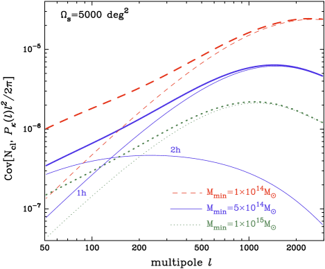
Figure 4: The cross-covariance between the cluster counts ${\cal N}$ and the lensing power spectrum $P^{\rm est}_{\kappa}(l)$ as a function of the angular multipole $l$ for a $\Lambda$CDM model. Note that for the purpose of this Figure we assume a single redshift bin for the lensing power spectrum for a typical ground-based survey (see § IV.1) and, for the cluster counts, we include all the clusters with masses above a given minimum halo mass over a range of redshifts $0\leq z\leq 1$. The dashed, solid and dotted curves demonstrate the results when minimum halo masses of $M_{\rm min}=1,5$ and $10\times 10^{14}M_{\odot}$ are employed, respectively. The two thin, solid curves show the 1- and 2-halo term contributions to the cross-covariance of $M_{\rm min}=5\times 10^{14}M_{\odot}$ (see Eqs. [LABEL:eqn:cpscov] and [LABEL:eqn:cov1h-2h]), while the thin dashed and dotted curves show the 1-halo term contribution.

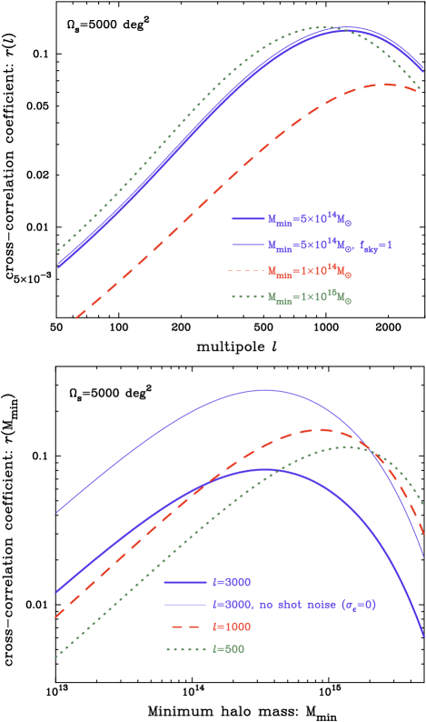
Figure 5: Upper panel: The cross-correlation coefficients, defined by Eq. (26), as a function of multipole $l$. The coefficient depends on the multipole bin width and survey area; we assumed $\delta l/l\simeq 0.04$ and $\Omega_{\rm s}=5000$ deg² ($f_{\rm sky}\simeq 0.12$), except for the thin solid curve where we assumed a full-sky survey $f_{\rm sky}=1$. Lower panel: A similar plot, but as a function of mass thresholds in the cluster counts, for a fixed multipole of the lensing power spectrum. The bold solid, dashed and dotted curves are the results for $l=3000$, $1000$ and $500$, respectively. The thin solid curve shows the result for $l=3000$ if the intrinsic ellipticity noise is ignored.

Fig. 4 shows the cross-covariance between the mass-selected cluster counts and the weak lensing power spectrum as a function of angular multipole $l$, for a concordance $\Lambda$CDM model. For illustrative clarity we use a single redshift bin for both of the cluster counts and the lensing power spectrum. The dashed, solid and dotted curves are the results obtained when minimum halo masses of $M_{\rm min}/10^{14}M_{\odot}=1,5$ and $10$ are assumed for the cluster counts, respectively. The two thin, solid curves show the 1- and 2-halo term contribution to the total power (bold solid curve) for the $M_{\rm min}/10^{14}M_{\odot}=5$ mass cut. It is apparent that the cross-covariance at small angular scales $l\lower 2.15277pt\hbox{$\;\buildrel>\over{\sim}\;$}500$ arises mainly from the 1-halo term contribution. Comparing the dashed, solid and dotted curves clarifies that the covariance amplitude gets greater with decreasing minimum halo mass, as the weak lensing and the cluster counts probe more similar density fields in the large-scale structure as implied in Fig. 3.

A more useful quantity is the cross-correlation coefficients defined as

$$r(l)=\frac{C^{gc}_{l1}}{\sqrt{C^{c}_{11}C^{g}_{ll}}},$$ (26)

where the subscript ‘$1$’ denotes the first redshift bin because for this calculation we are putting all the clusters into a single redshift bin, for illustration (the cluster redshift bin index $b=1$ for this case). The coefficients quantify the relative importance of the cross-covariance to the auto-covariances at a given $l$. The upper panel of Fig. 5 shows the correlation coefficients for model parameters assumed in Fig. 4. The coefficients depend on the multipole bin width taken in the lensing power spectrum covariance calculation as well as on a survey sky coverage; we here assumed $\Delta l/l\simeq 0.04$ and $\Omega_{\rm s}=5000$ deg², except for the thin solid curve where a full-sky survey $f_{\rm sky}=1$ is considered.

The upper panel of Fig. 5 shows that the coefficients peak around $l\sim 1000$, and decrease at smaller scales. On the intermediate scales there is a significant cross-correlation since the 1-halo term in the lensing power spectrum depends so strongly on the number of clusters (Fig. 3). However on smaller scales the lensing covariance is dominated by shot noise in the intrinsic galaxy shapes (e.g., see Fig. 1 in Jainetal07 ), which do not correlate with the cluster counts. Comparing the thin and bold solid curves shows that the coefficients have only weak dependence on the sky coverage, reflecting that the sampling variance of the cluster count covariance (19) roughly scales as $f_{\rm sky}^{-1}$ for a large area survey of our interest, which is same dependence as the other elements in the covariances.

The lower panel of Fig. 5 shows the correlation coefficients with varying mass thresholds in the cluster counts, for a fixed multipole $l$ of the lensing power spectrum. The lensing power spectrum at $l\sim 1000$ is found to be most correlated with the cluster counts for the $M_{\rm min}\sim 10^{15}M_{\odot}$ mass cut. The correlation decreases at high mass thresholds when the number of clusters is very small and therefore not representative of the lensing field. The correlation also decreases at smaller masses since the contribution to the lensing power spectrum is small for light halos (Fig 3). As can be seen from comparison of the bold and thin solid curves, an inclusion of the intrinsic ellipticity noise suppresses the correlation coefficients.

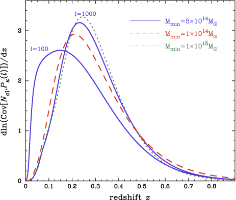
Figure 6: The relative contribution of each redshift clusters to the cross-covariance at a given multipole. We assumed the same model parameters as in Fig. 4. For an angular scale of $l=1000$, clusters at $z\sim 0.2$ most contribute to the cross-covariance, reflecting the peak of the lensing efficiency function. Note that we are here using the simple mass threshold for the cluster selection, not the lensing-based selection. On the other hand, for a larger angular scale of $l=100$, most of contribution comes from clusters at lower redshifts.

We now consider multiple redshift bins in the cluster catalog. Fig. 6 shows the relative contribution of each cluster count redshift bin to the cross-covariance at a given multipole. It is clear that clusters at $z\sim 0.2-0.3$ contribute most to the cross-covariance for an angular scale of $l\sim 1000$. Since the number density of mass-selected cluster counts has a weak redshift dependence as shown in Fig. 1, one can notice that the redshift peak reflects redshift dependence of the lensing efficiency function for a source redshift $z_{s}\sim 1$ that corresponds to the survey depth we assumed; structures at $z\sim 0.2-0.3$ most efficiently cause the lensing effect on source galaxies at $z_{s}\sim 1$. It is also worth noting that clusters at higher redshifts have a smaller angular size (smaller virial radii) than $\theta\sim 1/l$ (e.g. see the right panel of Fig. 2 in TJ03b ). In other words, clusters at $z\lower 2.15277pt\hbox{$\;\buildrel>\over{\sim}\;$}0.5$ may carry complementary information to the lensing power spectrum. On the other hand, for an angular scale of $l\sim 100$, clusters at lower redshifts $z\sim 0.1$ contribute most to the covariance, because the cluster virial radius matches such a large angular scale only if the cluster is located at lower redshift.

IV Results: Signal-to-Noise and Parameter Forecasts

IV.1 A CDM model and survey parameters

To compute the observables of interest we need to specify cosmological model and we assume survey parameters similar to those of future surveys in order to estimate realistic measurement errors.

We include the key parameters that may affect the observables within an adiabatic CDM dominated model with dark energy component: the density parameters are $\Omega_{\rm de}(=0.73)$, $\Omega_{\rm m}h^{2}(=0.14)$, and $\Omega_{\rm b}h^{2}(=0.024)$ (note that we assume a flat universe); the primordial power spectrum parameters are the spectral tilt, $n_{s}(=1)$, the running index, $\alpha_{s}(=0)$, and the normalization parameter of primordial curvature perturbation, $\delta_{\zeta}(=5.07\times 10^{-5})$ (the values in the parentheses denote the fiducial model). We employ the transfer function of matter perturbations, $T(k)$, with baryon oscillations smoothed out EisensteinHu99 . We employ the dark energy model ChevallierPolarski01 ; Linder03 parametrized as $w(a)=w_{0}+w_{a}(1-a)$, with fiducial values $w_{0}=-1$ and $w_{a}=0$.

We specify survey parameters that well resemble a future ground-based survey (e.g., see HSC ). We model the redshift distribution of galaxies by using a toy model given by Eq. (4) in Hutereretal06 ; we employ the parameter value $z_{0}=0.3$ leading the redshift distribution to peak at $z_{\rm peak}=2z_{0}=0.6$ and have a mean redshift of $z_{\rm m}=3z_{0}=0.9$. The intrinsic ellipticities dilute the lensing shear measurements according to Eq. (17); we simply assume that the shot noise contamination is modeled by the rms ellipticity per component, $\sigma_{\epsilon}=0.22$, and the total number density of galaxies, $\bar{n}_{g}=30$ arcmin^-2. The survey area is taken to be $\Omega_{\rm s}=5000$ degree² for our fiducial choice. Note that throughout this paper we will assume that the two observables we are interested in, the cluster number counts and the lensing power spectrum, are taken from the same survey region, to study how the cross-correlation affects the parameter constraints. as the two methods probe the same cosmic structure.

IV.2 A signal-to-noise ratio

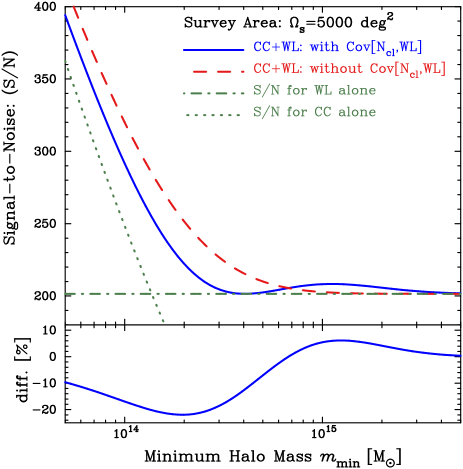
Figure 7: Upper panel: Signal-to-noise ($S/N$) ratio as a function of the mass threshold of the cluster count measurement. The solid curve shows the total $S/N$ for a combined measurement of the cluster counts and lensing power spectrum where the cross-correlation between the two observables, ${\rm Cov}[{\cal N}_{\rm cl},P_{\kappa}(l)]$, is included. For comparison, the dashed curve shows the $S/N$ assuming that the two observables are independent (i.e. the cross-correlation is ignored). The dotted and dot-dashed curves show the $S/N$ when either of the cluster counts or the lensing power spectrum alone is considered. Lower panel: The percentage difference in $S/N$ with and without the cross-covariance ${\rm Cov}[{\cal N}_{\rm cl},P_{\kappa}(l)]$ (i.e., the difference between the solid and dashed curves divided by the dashed curve in the upper panel $\times 100$). Interestingly, the cross-correlation improves the $S/N$ by up to $10\%$ when only massive clusters with $M\lower 2.15277pt\hbox{$\;\buildrel>\over{\sim}\;$}10^{15}M_{\odot}$ are included in the counts (see text for a more detailed discussion). All curves assume a survey with an area of $\Omega_{s}=5000$ deg². Note that we considered a single redshift bin for both of the two observables, and included the number counts of clusters with masses greater than the mass threshold over redshifts $0.05\leq z\leq 1.0$ and the lensing power spectrum at multipoles over $50\leq l\leq 3000$, respectively (see text for the details).

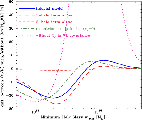
Figure 8: Shown is the relative importance of each ingredient in the covariance calculation to the percentage difference in $S/N$. The solid curve shows the result for our fiducial model, as shown in the lower panel of Fig. 7. The dashed curve shows the results where only the 1-halo terms are included in each element of the full covariance matrix, while the thin dashed curve shows the results when only the 2-halo term contribution to the cross-covariance is included. The dotted and dot-dashed curves show the results when the intrinsic ellipticity noise or the non-Gaussian errors are ignored in the weak lensing power spectrum covariance, respectively.

It is instructive to investigate the expected signal-to-noise ($S/N$) ratio for a combined measurement of the cluster counts and the lensing power spectrum, in order to highlight how the cross-correlation between the two observables affects the measurement accuracies. The $S/N$ can be estimated using the covariance matrix derived in § III as

$$\left(\frac{S}{N}\right)^{2}_{c+g}\equiv\sum_{i,j}D_{i}\left[(\bm{C}^{g+c})^{-1}\right]_{ij}D_{j}.$$ (27)

Here the data vector of our observables, $\bm{D}$, constructed from the lensing power spectrum tomography with $n_{s}$ redshift bins and the cluster number counts with $b$-redshift bins is defined as

$$\bm{D}=\left\{{P_{(11)\kappa}(l_{1}),\cdots,P_{(n_{s}n_{s})\kappa}(l_{\rm max})},N_{(1)},\cdots,N_{(b)}\right\}.$$ (28)

Note that the dimension of $\bm{D}$ is $b+n_{l}\times n_{s}(n_{s}+1)/2$ when the lensing tomography with $n_{l}$ multipole bins and $n_{s}$ redshift bins and the cluster counts with $b$ redshift bins are considered (also see below Eq. [22]). For a case of $b=10$, $n_{s}=3$ and $n_{l}=100$, the dimension of $\bm{D}$ is 610. The full covariance matrix for the joint measurement, $\bm{C}^{c+g}$, can be constructed from Eqs. (19), (LABEL:eqn:pscov), and (LABEL:eqn:cpscov) as

$$\bm{C}^{g+c}\equiv\left(\begin{array}[]{cc}\bm{C}^{g}&\bm{C}^{gc}\\ \bm{C}^{gc}&\bm{C}^{c}\\ \end{array}\right).$$ (31)

Note that $(\bm{C}^{g+c})^{-1}$ appearing in Eq. (27) is the inverse matrix of $\bm{C}^{g+c}$.

For comparison we consider the $S/N$ from each of cluster counts and weak lensing alone by using the relevant part of the data vector in Eq. (28) and the covariance matrices. We also compare with the $S/N$ if the cross-correlation is not taken into account, i.e. a matrix of zeros is used instead of the matrix $\bm{C}^{gc}$ in Eq. (31). In this case that the two are independent, e.g. measured from non-overlapping two survey regions, the $S/N$ values from each of the cluster counts and the lensing power spectrum alone therefore add in quadrature to form the joint $S/N$.

When computing $S/N$ in Eq. (27) care must be taken with numerical accuracy of the matrix inversion. The observables of interest, the angular number density of clusters and the lensing power spectrum, have different units and their amplitudes could therefore differ from each other by many orders of magnitudes. To avoid numerical inaccuracies caused by this fact, we have used the dimension-less covariance matrix $\tilde{\bm{C}}^{g+c}$ normalized by the data vector as

$$\left[\tilde{\bm{C}}^{g+c}\right]_{ij}\equiv\frac{\left[\bm{C}^{g+c}\right]_{ij}}{D_{i}D_{j}}.$$ (32)

In terms of the re-defined covariance matrix, the total $S/N$ can be computed simply as $(S/N)_{g+c}^{2}=\sum_{i,j}[\tilde{\bm{C}}^{g+c}]^{-1}_{ij}$.

Fig. 7 shows the $S/N$ ratios expected for a ground-based survey with area $\Omega_{\rm s}=5000$ deg² and our fiducial $\Lambda$CDM model, as a function of minimum halo mass used in the mass-selected cluster counts. Here we include all the clusters with masses greater than a given mass threshold over a range of $0.05\leq z\leq 1$, and include the lensing power spectrum at multipoles $50\leq l\leq 3000$ assuming the redshift distribution of galaxies described in § IV.1. Note that we here consider a single redshift bin for both the cluster counts and cosmic shear power spectrum for simplicity, and the signal-to-noise ratios only slightly increase by adding redshift binned information (e.g., see Fig. 5 in TJ04 ). First of all, we should notice that the lensing power spectrum and the cluster number counts have similar $S/N$ ratios, when the mass threshold $M_{\rm min}\sim 10^{14}M_{\odot}$ is used. At mass thresholds smaller than $10^{14}M_{\odot}$, the cluster counts (dotted curve) have a greater $S/N$ than the lensing power spectrum (dot-dashed curve) due to an increase in the number of sampled clusters, while the lensing power spectrum has a greater $S/N$ at the greater mass threshold.

The solid curve shows the total $S/N$ for a combined measurement of the cluster counts and the lensing power spectrum, when the cross-correlation between the two observables is correctly taken into account for the full covariance matrix (see Eq. [31]). We compare this to the standard approach in which the two probes are considered to be independent (dashed curve). The lower panel explicitly shows the percentage difference in $S/N$ with and without the cross-covariance.

At small mass thresholds $\lower 2.15277pt\hbox{$\;\buildrel<\over{\sim}\;$}10^{14}M_{\odot}$, the total $S/N$ taking into account the cross-covariance is degraded compared to when the probes are considered independent. This is because the cosmic density field probed is shared by the two observables and therefore an inclusion of the cross-covariance reduces independence of the two observables. However, the degradation ceases at a critical mass scale where the total $S/N$ (including the covariance) is equal to the $S/N$ for the lensing power spectrum alone. In other words, the total $S/N$ is never smaller than the $S/N$ obtained from either alone of the lensing power spectrum or the cluster counts.

Then, an intriguing result is found: the total $S/N$ is slightly improved by including the cross-covariance as the mass threshold is increased up to $M\sim 10^{15}M_{\odot}$, where the improvement is up to $\sim 10\%$ as shown in the lower panel. This occurs even though the $S/N$ ratio from the cluster counts alone is much less than that for the lensing power spectrum alone. The peak mass scale of the total $(S/N)$ corresponds to the mass scale at which the correlation coefficient of the covariance peaks as can be found in the lower panel of Fig. 5. That is, the improvement in $S/N$ could happen when the two observables are highly correlated. Since the cross-covariance describes how the two observables are correlated with each other, it appears that a knowledge of the number of such massive clusters with $M\lower 2.15277pt\hbox{$\;\buildrel>\over{\sim}\;$}10^{15}M_{\odot}$ for a given survey region helps to improve the amount of information that can be extracted from the weak lensing measurement (also see Neyrincketal06 ; NeyrinckSzapudi07 for the related discussion). In simpler words, if a smaller or greater number of massive clusters than the ensemble average value was observed from a given survey region, the observed lensing power spectrum will most likely have smaller or greater amplitudes at $l\sim 10^{3}$, respectively.

We reproduce this qualitative behavior using a simple toy model described in the Appendix C, where the lensing power spectrum is modeled to be given solely by the number of halos, ignoring the halo mass profile and the clustering of different halos. Based on this toy model we attribute the increase in the total $S/N$ for high cluster mass thresholds to the fact that the lensing power spectrum amplitude is sensitive to the number of such massive clusters as demonstrated in Fig. 3. The fact that the lensing power spectrum is sensitive to the number counts weighted by the mass squared, means that it adds complementary information to the unweighted sum from the cluster counts.

It should, however, be noted that the improvement in $S/N$ is achievable only if the cross-covariance is a priori known from the theoretical prediction e.g. based on CDM structure formation scenarios. Alternatively it could be obtained from a measurement of the cross-correlation from the survey region.

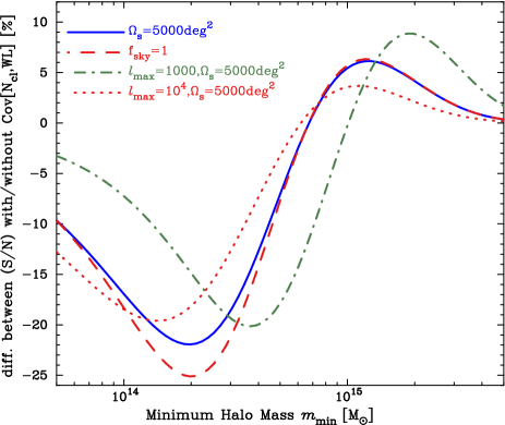
Figure 9: Dependence of the percentage difference in $S/N$ (see lower panel of previous plot) on survey area and maximum multipole $l_{\rm max}$, where information on the lensing power spectrum over a range of $50\leq l\leq l_{\rm max}$ is included. The default is $l_{\rm max}=3000$.

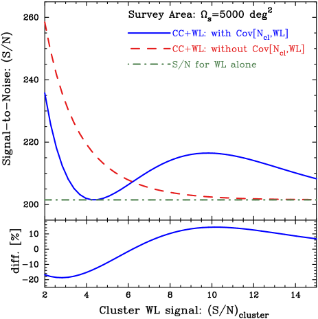
Figure 10: As in Fig. 7, but the total signal-to-noise for the lensing-based cluster counts (see Fig. 2) combined with the lensing power spectrum measurement is shown against detection thresholds of the cluster lensing signal (see Eq. [6]). Note that the plotting range of $y$-axis in the upper panel is smaller than that of Fig. 7.

In Fig. 8 we study which model ingredient in the full-covariance calculation mainly leads to the results in Fig. 7. The dashed curve shows the percentage difference in $S/N$ when only the 1-halo terms are included in each element of the full covariance matrix (31), which corresponds to a simplified case that there is no clustering between halos. Compared to the solid line, or Fig. 7, the results are little different. The dot-dashed curve shows the result obtained when we ignore the intrinsic ellipticity noise that contributes only to the diagonal elements of the weak lensing power spectrum covariance. Again only a small difference is found. On the other hand, the thin dashed curve shows the results when only the 2-halo term contribution to the cross-covariance is included, which attempts to reproduce the results in the previous work FangHaiman06 . For this case, the impact of the cross-covariance on the $S/N$ is negligible as concluded in FangHaiman06 . Rather, it turns out that the most important effect comes from the lensing trispectrum contribution to the lensing power spectrum covariance. If we switch off the non-Gaussian contribution, the percentage difference in $S/N$ is significantly changed. In particular, there is a significant improvement in $S/N$ by adding the cluster counts with $M\lower 2.15277pt\hbox{$\;\buildrel>\over{\sim}\;$}10^{15}M_{\odot}$, because ignoring the lensing trispectrum decreases the diagonal elements in the full covariance matrix and thus enhances the relative importance of the cross-covariance. This also implies that the cosmic shear fields are highly non-Gaussian as carefully investigated in TJ07 .

Fig. 9 demonstrates how this percentage difference in $S/N$ depends on the sky coverage ($f_{\rm sky}$) and the maximum multipole ($l_{\rm max}$) of the lensing power spectrum. All the curves in Fig. 9 are very similar, showing a weak dependence on $f_{\rm sky}$ and $l_{\rm max}$. (Note however that the absolute $S/N$ itself has a strong dependence.) Nevertheless, there are several points to note when interpreting the results. Comparing the dotted, solid and dot-dashed curves clarify that, with increasing $l_{\rm max}$, the mass threshold corresponding to the dip in the percentage difference in $S/N$ increases. This is because the lensing power spectrum at higher multipoles is more sensitive to the cosmic density fields down to smaller length scales, and therefore the cluster counts including less massive halos are more correlated with the lensing power spectra. Also the impact of the cross-covariance is reduced when assuming $l_{\rm max}=10^{4}$, compared to the fiducial case of $l_{\rm max}=3000$, because the intrinsic ellipticity noise (shot noise) is dominant in the lensing power spectrum covariance at such small scales.

Similar to Fig. 7, Fig. 10 shows the total $S/N$ ratios for a combined measurement of the lensing-based cluster counts and the lensing power spectrum, as a function of the cluster lensing-signal thresholds (see Eq. [6] and Fig. 2). Notice that the plotting range of $y$-axis is roughly half of that in Fig. 7. Because the number densities for the lensing signal thresholds of interest are less than that for the mass-selected cluster sample (as shown in Fig. 2) the lensing-based cluster counts do not contribute much to the total $S/N$ ratios, compared to Fig. 7. Other than this difference, the behavior for the $S/N$ curves found in Fig. 7 are similar to those in Fig. 10.

IV.3 Fisher analysis for cosmological parameter constraints

We now estimate accuracies of cosmological parameter determination, given the measurement accuracies of the observables, using the Fisher matrix formalism Fisher35 ; Tegmarketal97 . This formalism assesses how well given observables can constrain cosmological parameters around a fiducial cosmological model. The parameter forecasts we obtain depend on the fiducial model and are also sensitive to the choice of free parameters. Furthermore, the Fisher matrix gives only a lower limit to the parameter uncertainties, being exact if the likelihood surface around the local minimum is Gaussian in multi-dimensional parameter space. Ideally a more quantitative method would be used to explore the global structure to realize more accurate parameter forecasts. As described in § IV.1, we include all the key parameters that can describe varieties in the observables within $\Lambda$CDM model cosmologies.

The Fisher information matrix available from the lensing power spectrum tomography is given by

$$[\bm{F}^{g}]_{\alpha\beta}=\sum_{m,n}\frac{\partial P_{(ij)\kappa}(l_{a})}{\partial p_{\alpha}}\left[\bm{C}^{g}\right]^{-1}_{mn}\frac{\partial P_{(ij)\kappa}(l_{b})}{\partial p_{\alpha}},$$ (33)

where the partial derivative with respect to the $\alpha$-th cosmological parameter $p_{\alpha}$ is evaluated around the fiducial model, with other parameters $p_{\beta}$ ($\alpha\neq\beta$) being fixed to their fiducial values. The error on a parameter $p_{\alpha}$, marginalized over other parameter uncertainties, is given by $\sigma^{2}(p_{\alpha})=(\bm{F}^{-1})_{\alpha\alpha}$, where $\bm{F}^{-1}$ is the inverse of the Fisher matrix.

Similarly, the Fisher matrix for the cluster counts is given by

$$[\bm{F}^{c}]_{\alpha\beta}=\sum_{b,b^{\prime}}\frac{\partial N_{(b)}}{\partial p_{\alpha}}\left[\bm{C}^{c}\right]^{-1}_{bb^{\prime}}\frac{\partial N_{(b^{\prime})}}{\partial p_{\alpha}}.$$ (34)

For a combined measurement of the lensing power spectrum and the cluster counts, the Fisher matrix is calculated using the full covariance matrix defined by Eq. (31) (also see Eq. [32]) as

$$[\bm{F}^{g+c}]_{\alpha\beta}=\sum_{i,j}\frac{\partial\ln D_{i}}{\partial p_{\alpha}}\left[(\tilde{\bm{C}}^{g+c})^{-1}\right]_{ij}\frac{\partial\ln D_{j}}{\partial p_{\alpha}},$$ (35)

where the summation indices $i,j$ run over the redshift and multipole bins of the tomographic lensing power spectra as well as the redshift bins of the cluster counts.

Using probes of structure formation alone is not powerful enough to constrain all the cosmological parameters simultaneously and well. Rather, combining the large-scale structure probes with constraints from CMB temperature and polarization anisotropies significantly helps to lift parameter degeneracies and, in particular, the dark energy parameters (e.g. Eisensteinetal99 ; TJ04 ). When computing the Fisher matrix for a given CMB data set, we employ 9 parameters: the 8 parameters described in § IV.1 plus the Thomson scattering optical depth to the last scattering surface, $\tau(=0.10)$. Note that we ignore the contribution to the CMB spectra from the primordial gravitational waves for simplicity. We use the publicly-available CMBFAST code SeljakZaldarriaga96 to compute the angular power spectra of temperature anisotropy, $C^{\rm TT}_{l}$, $E$-mode polarization, $C^{\rm EE}_{l}$, and their cross-correlation, $C^{\rm TE}_{l}$. To model the measurement accuracies we assume the noise per pixel and the angular resolution of the Planck experiment that were assumed in Eisensteinetal99 .

To be conservative, however, we do not include the CMB information on the dark energy equation of state parameters, $w_{0}$ and $w_{a}$. We do this because essentially angular positions of the CMB acoustic peaks constrain a degenerate combination of the curvature of the universe and the dark energy parameters, through their dependences on the angular diameter distance to the last scattering surface. We are assuming a flat universe and therefore wish to remove the artificially good constraint on dark energy that we would get from the CMB. Note, however, that our parameter forecasts shown below would not change significantly even for a non-flat universe, because we focus on large-scale structure probes in combination with the CMB constraints, as carefully shown in Knoxetal06 .

We remove the CMB information on the dark energy parameters using the following steps. We first compute the inverse of the CMB Fisher matrix, $\bm{F}^{-1}_{\rm CMB}$, for the 9 parameters in order to obtain marginalized errors on the parameters, and then re-invert a sub-matrix of the inverse Fisher matrix that includes only the rows and columns for the parameters besides $w_{0}$ and $w_{a}$. The sub-matrix of the CMB Fisher matrix derived in this way describes accuracies of the 7 parameter determination, having marginalized over degeneracies of the dark energy parameters $w_{0}$ and $w_{0}$ with other parameters for the hypothetical Planck data sets. In addition, we use only the CMB information in the range of multipoles $10\leq l\leq 2000$, and therefore we do not include the integrated Sachs-Wolfe (ISW) effect that contribute to the CMB spectra mainly at low multipoles $l\lower 2.15277pt\hbox{$\;\buildrel<\over{\sim}\;$}10$, because the ISW effect is very likely correlated with the cosmic shear power spectrum and cluster counts, and we will ignore the correlations in this paper.

To obtain the Fisher matrix for a joint experiment combining the lensing and/or cluster experiments with the CMB information, we simply sum the two Fisher matrices as, e.g. $\bm{F}^{g+c+{\rm CMB}}=\bm{F}^{g+c}+\bm{F}^{\rm CMB}$ because the CMB information can be safely considered as an independent probe to the low-$z$ universe probes in our setting. Note that the final Fisher matrix such as $\bm{F}^{g+c+\rm CMB}$ has $9\times 9$ dimensions.

IV.4 Forecasts for parameter constraints

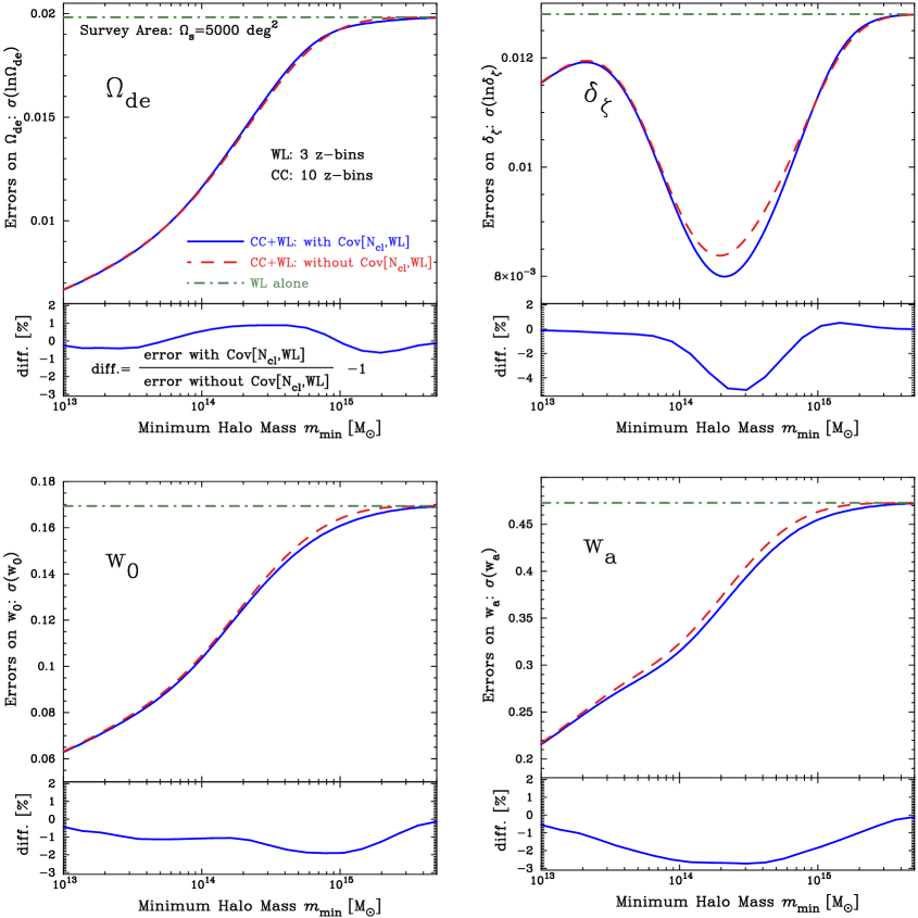
Figure 11: The projected $68\%$ C.L. error on each of the parameters, $\Omega_{\rm de}$ (upper-left panel), $\delta_{\zeta}$ (upper-right), $w_{0}$ (lower-left) and $w_{a}$ (lower-right), marginalized over other parameters (9 parameters in total), as a function of mass thresholds used in the cluster counts. We assume 10 redshift bins for the cluster counts over redshifts $0.05\leq z\leq 1.0$, and 3 redshift bins for the lensing power spectrum tomography assuming the redshift distribution of galaxies described in § IV.1, for a survey of 5000 deg² area. In the upper panel of each plot, the solid curve shows the errors expected from a combined measurement of the cluster counts and the lensing tomography when the cross-covariance between the two observables are correctly taken into account, while the dot-dashed curves shows the errors for the lensing tomography alone. The dashed curve shows the error from combining cluster counts and lensing tomography when the cross-covariance is ignored. Note that all the results shown here assume the Planck priors discussed in § IV.3. The lower panel of each plot shows the percentage difference in the parameter errors with and without the cross-covariance, highlighting the impact of the cross-covariance on the parameter forecasts. The errors on the dark energy equation of state parameters, $w_{0}$ and $w_{a}$, are improved by an inclusion of the cross-covariance over mass thresholds we have considered, but the effect is small (only a few %).

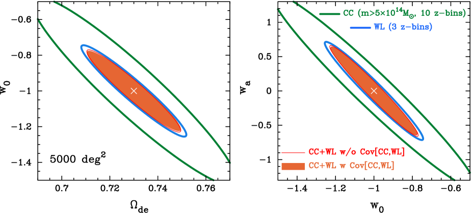
Figure 12: As in Fig. 11, but this plot explicitly shows projected 68% error ellipses in two-parameter subspace the dark energy parameters $(\Omega_{\rm de},w_{0},w_{a})$, for cluster counts of mass cut $M_{\rm min}=5\times 10^{14}M_{\odot}$. The outermost and middle bold-solid curves in each panel are the error ellipses expected when using either alone of the cluster counts or the lensing power spectrum tomography in combination with Planck, while the innermost shaded ellipses show the errors for the two observables combined. For comparison, the thin-solid curves show the error ellipses obtained when ignoring the cross-covariance; the effect is very small (the area is enlarged only by a few $\%$). The cross symbol in each plot shows the fiducial model for the Fisher matrix analysis.

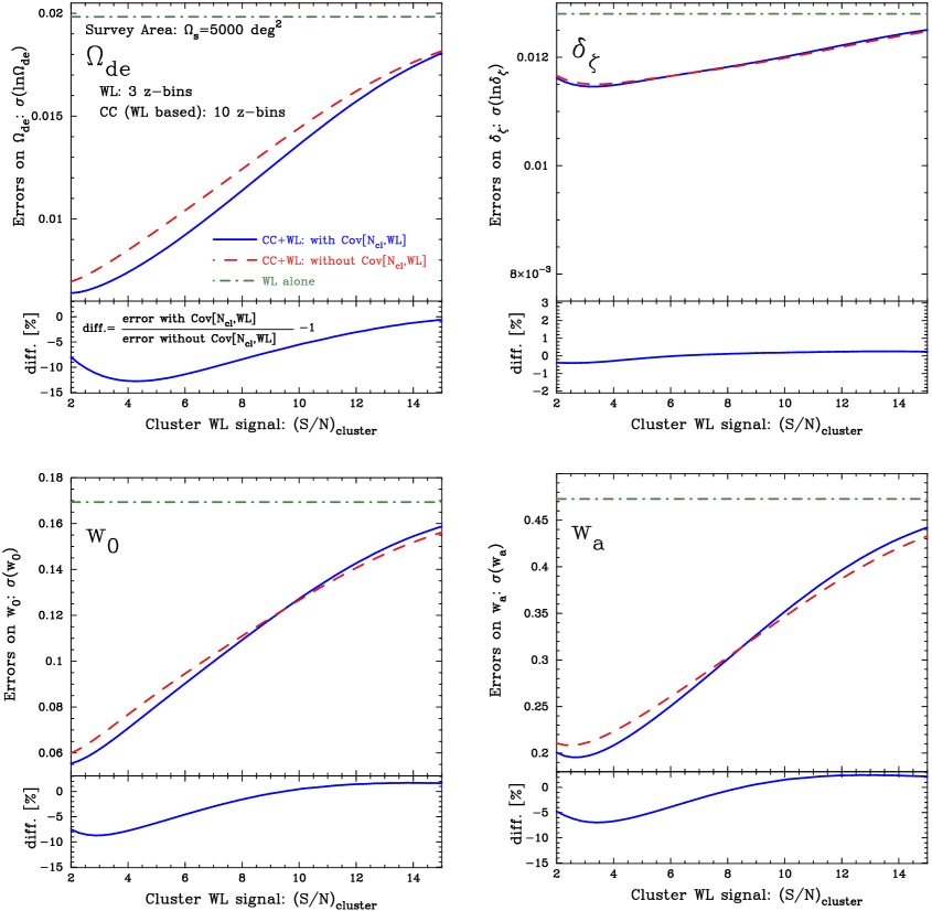
Figure 13: Similar to the previous plot, but for the lensing-based cluster counts as a function of the detection thresholds, where clusters having the lensing signal greater than the threshold are included in the counts. Note that the plotting range of $y$-axis in the upper panel of each plot is same as that in Fig. 11. A similar improvement in the parameter error is obtained by adding the cluster counts, even though the lensing based cluster counts generally contain fewer clusters than the mass-selected cluster counts as shown in Fig. 2. The inclusion of the covariance between cluster counts and lensing tomography is slightly larger here, compared to when a mass threshold is used for the cluster counts.

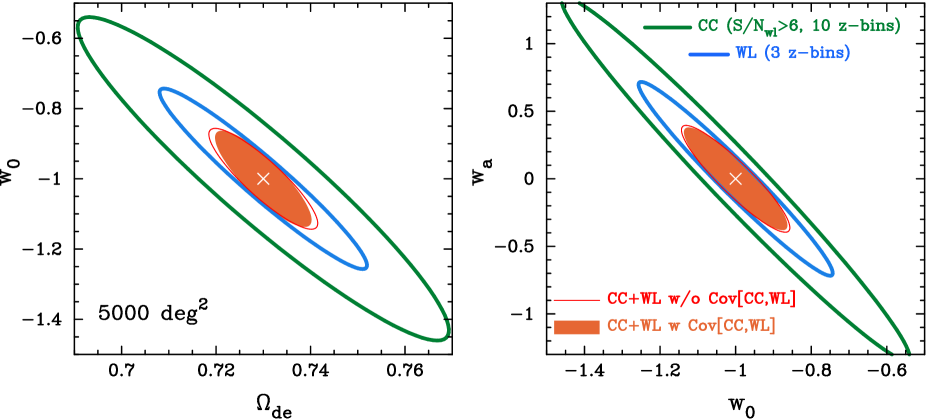
Figure 14: As in Fig. 12, but for the lensing-based cluster counts of detection threshold $(S/N)_{\rm cluster}=6$.

When forecasting cosmological parameter determination, we should notice that the redshift information inherent in the cluster number counts and the lensing power spectrum can be very powerful to significantly tighten cosmological parameter errors, especially dark energy parameters (e.g., see TJ04 ). In the following, we will assume $3$ redshift bins for lensing tomography and $10$ redshift bins for the cluster number counts over $0.05\leq z\leq 1.0$, for a survey with 5000 deg² area. The ‘three’ redshift bins for lensing tomography is a minimal choice to obtain non-degenerate constraints on the ‘three’ dark energy parameters, $\Omega_{\rm de}$, $w_{0}$ and $w_{a}$ as implied from Fig. 3 in Maetal05 , although four or more redshift bins lead to further improvement, albeit not so much, in the parameter errors. Since we ignore various systematic errors for both the cluster counts and the lensing tomography, we adopt a rather conservative setting for the lensing tomographic binning. However note that we have checked a different redshift binning for cluster counts in combination with the lensing tomography does not change the main results below significantly. An investigation into survey optimization for survey parameters (area and depth) and redshift binning will be presented elsewhere in a more practical manner taking into account possible effects of the systematic errors.

We first consider mass-selected cluster counts, and Fig. 11 shows the expected $68\%$ limits on each of the parameters $\Omega_{\rm de}$, $\delta_{\zeta}$, $w_{0}$ and $w_{a}$, as a function of mass thresholds in the cluster counts. In each case we have marginalized over the remaining 8 cosmological parameters (see § IV.1 and  IV.3 for the cosmological parameters used). It should be also noted that the errors on these 4 parameters are enlarged only by $\sim 10\%$ without the CMB priors. In the upper panel of each plot, the solid curve shows the error on a given parameter when the cross-covariance between the two observables is correctly taken into account, while the dot-dashed curve shows the error obtained from the lensing tomography alone. Comparing the solid and dot-dashed curves demonstrates that adding the cluster counts for the smaller mass cuts into the lensing tomography can more improve the errors on dark energy parameters, $\Omega_{\rm de}$, $w_{0}$ and $w_{a}$, because the two observables depend on cosmological parameters in different ways and combining the two can lift the parameter degeneracies (also see FangHaiman06 ). To be more explicit, the errors are improved by $\sim 40\%$ for mass threshold $M_{\rm min}\sim 10^{14}M_{\odot}$, while the errors are improved only slightly by $\sim 5\%$ for $M_{\rm min}\sim 10^{15}M_{\odot}$.

On the other hand, there is a complex behavior in the error on the primordial curvature perturbation, $\delta_{\zeta}$. This is explained as follows. The cluster counts are very sensitive to the normalization parameter of the linear mass power spectrum ($\delta_{\zeta}$ for our case or $\sigma_{8}$ often used in the literature) through the sharp exponential cut-off of the halo mass function at high mass end. As we reduce the minimum mass threshold down to the range $3\times 10^{13}\lower 2.15277pt\hbox{$\;\buildrel<\over{\sim}\;$}M_{\rm min}/M_{\odot}\lower 2.15277pt\hbox{$\;\buildrel<\over{\sim}\;$}10^{14}$ we are beginning to lose information about the number of very high mass clusters, which are diluted in the total count by the large number of low mass clusters. At much lower mass cuts $M_{\rm min}\lower 2.15277pt\hbox{$\;\buildrel<\over{\sim}\;$}3\times 10^{13}M_{\odot}$, the cluster counts come back to yield a tighter constraint on $\delta_{\zeta}$ than the lensing tomography through the better measurement accuracy due to the larger number of very low mass halos. It would be also worth pointing out that knowing the number of clusters can effectively allow the lensing power spectrum to yield more information on the linear theory part of the power spectrum (e.g. one could subtract off the contribution from the clusters to get at the two halo term). Therefore the constraint on the power spectrum amplitude can be partly improved from the joint constraint from the mass function and the linear power spectrum. Note that in this paper we consider a simple mass threshold for the cluster counts, however if clusters can be binned by mass then the information would be restored and we may also use the shape of the mass function to constrain cosmological parameters (e.g. Rozoetal07 ).

The impact of the cross-covariance between the two observables on the parameter forecasts can be found from comparison of the solid and dashed curves: the dashed curve shows the error obtained when the two observables are considered to be independent. Further, the lower panel of each plot explicitly presents the percentage difference in the errors. The impact of the cross-covariance on the parameter errors is generally very small, at only a few per cent.

Nevertheless, interestingly, in some cases an inclusion of the cross-covariance leads to an improvement in the parameter errors; for example, the errors on $w_{0}$ or $w_{a}$ are improved over a range of the mass thresholds we have considered. This perhaps counter-intuitive result is in part due to working in 9 dimensional parameter space, and could also be explained as follows (also see TJ07 for related discussion). As we have carefully investigated, the cross-covariance predicted from a CDM model quantifies how the cluster counts and the lensing power spectrum amplitude are correlated with each other in redshift and multipole space. The positive cross-correlation shown in Fig. 4 implies that for a given survey region, if the number of clusters probed happens to be higher or lower than the ensemble average, the lensing power spectrum will be expected to have larger or smaller amplitudes, respectively. Therefore, such a correlated offset in the two observables makes it difficult to determine their true amplitudes compared to the case in which the two observables are independent, thereby degrading the errors of parameters that are primarily sensitive to the amplitudes of the two observables. This explains the degradation in the errors on $\Omega_{\rm de}$ and $\delta_{\zeta}$ for some range of mass thresholds. On the other hand, the correlated offset rather preserves relative values between the cluster counts and the lensing spectrum amplitudes in redshift and multipole space. That is, a priori knowledge on the cross-covariance leads to an improvement in the errors on parameters that imprint characteristic redshift and multipole dependences onto the cluster counts and the lensing power spectrum. This is the case for the parameters $w_{0}$ and $w_{a}$.

In Fig. 12 we show the projected 68% C.L. error ellipses in the dark energy parameter space, for one particular example mass threshold, $M_{\rm min}=5\times 10^{14}M_{\odot}$. The error ellipses in a two-parameter subspace highlight how the two parameters considered are degenerate for a given observable and the degeneracies are broken by combining different observables. It can be seen that the lensing power spectrum tomography and the cluster counts have similar degeneracy directions in constraining the dark energy parameters. Adding the cluster counts only slightly improves the parameter errors compared to the errors from the lensing tomography alone. The plot also shows that the cross-covariance has a negligible effect on the error ellipses.

Fig. 13 shows the results for the lensing-based cluster counts, as a function of the cluster lensing signal, where clusters having a lensing signal greater than a given threshold, $(S/N)_{\rm cluster}$, are included in the counts. As in Fig. 11, we consider $10$ redshift bins for the cluster counts over redshifts $0.05\leq z\leq 1$ and $3$ redshift bins for the lensing tomography. Note that the plotting range of $y$-axis in the upper panel of each plot is same as that in Fig. 11, while the plotting range in the lower panel is different.

First of all, it should be noted that adding the lensing-based cluster counts into the lensing tomography does tighten the errors on $\Omega_{\rm de}$, $w_{0}$ and $w_{a}$ significantly even though the cluster counts include fewer clusters than the mass-selected counts (see Fig. 2). For the threshold $(S/N)_{\rm cluster}\sim 10$, which includes clusters with masses $M\lower 2.15277pt\hbox{$\;\buildrel>\over{\sim}\;$}10^{15}M_{\odot}$ and mainly covers a narrow redshift range of $0.05\lower 2.15277pt\hbox{$\;\buildrel<\over{\sim}\;$}z\lower 2.15277pt\hbox{$\;\buildrel<\over{\sim}\;$}0.6$, the cluster counts still improve the dark energy parameters by $\sim 25\%$, in contrast with only $\sim 4\%$ improvement for the mass-selected cluster counts with $M\lower 2.15277pt\hbox{$\;\buildrel>\over{\sim}\;$}10^{15}M_{\odot}$ in Fig. 11. We find the same percentage improvement when the CMB priors are not included. With the reasonable value of $(S/N)_{\rm cluster}\sim 6$ the uncertainties are halved by adding cluster counts to lensing power spectra. The relatively amplified sensitivity to dark energy is attributed to the fact that the cluster lensing signal itself depends on the dark energy parameters via the lensing efficiency, even for a fixed halo mass (see Eq. [6]).

For the primordial curvature perturbation $\delta_{\zeta}$, adding the cluster counts does not improve the error much, compared to the result in Fig. 11. The parameter $\delta_{\zeta}$ does not affect the amount of lensing for a given cluster so the poorer accuracy just arises from larger statistical errors due to the smaller number of clusters, compared to the mass-selected counts.

As shown in the lower panel of each plot, the cross-covariance has more influence on the parameter forecasts, compared to Fig. 11. This is because lensing-based cluster counts and lensing tomography both pick up halos over a very similar range in redshifts. Therefore there are more significant cross-correlations between the two observables. However, the effect of the cross-covariances on the parameter errors is small, by less than $\sim 10\%$, for $(S/N)_{\rm cluster}\lower 2.15277pt\hbox{$\;\buildrel>\over{\sim}\;$}6$.

Fig. 14 shows the marginalized error ellipses, for the lensing-signal detection threshold $(S/N)_{\rm cluster}=6$. The degeneracy directions in dark energy parameter constraints are very similar between the cluster counts and the lensing tomography. Compared to Fig. 12, the lensing-based cluster counts have a better accuracy of constraining the dark energy parameters, thereby leading the error ellipses to more shrink when the cluster counts and the lensing tomography combined. This can be explained because the contours in the dark energy equation of state parameter space is just a projection of the full 9d space. We have investigated eigendirections in cosmological parameter space and identified differences between cluster counts and lensing for $\delta_{\zeta}$ and $\Omega_{m}h^{2}$ (effectively $h$ given that $\Omega_{m}$ is a parameter in the Fisher matrix). For example, we find that if we plot $w_{0}$ against $\delta_{\zeta}$ then we see that the cluster counts plus CMB contours are more aligned with the $w_{0}$ axis whereas the lensing plus CMB contours are more aligned with the $\delta_{\zeta}$ axis. When combined together, both degeneracies are broken and the error bar on $w_{0}$ is reduced. Similarly for $\delta_{\zeta}$ and $w_{a}$ and $\Omega_{m}h^{2}$ with each dark energy parameter. This explains why the combined contours (cluster counts plus lensing plus CMB) are smaller than either separate contour (cluster counts plus CMB or lensing plus CMB), even though the separate constraints have the same degeneracy directions when projected down onto $w_{0}$ versus $w_{a}$ space.

Probes	$\sigma(\Omega_{\rm de})$	$\sigma(\ln\delta_{\zeta})$	$\sigma(w_{\rm piv})$	$\sigma(w_{a})$	$\sigma(w_{\rm piv})\times\sigma(w_{a})$
WLT	0.014	0.013	0.039	0.47	0.019
CCM ($M_{\rm min}=5\times 10^{14}M_{\odot}$)	0.028	0.015	0.085	0.95	0.081
WLT+CCM	[0.013]	[0.0096]	[0.033]	[0.44]	[0.0143]
WLT+CCM (with cross-cov.)	0.013 ($0\%$)	0.0093 ($3\%$)	0.032 ($3\%$)	0.42 ($3\%$)	0.0135($6\%$)
CCWL ($(S/N)_{\rm cluster}\geq 6$)	0.026	0.015	0.061	0.89	0.054
WLT+CCWL	[0.0076]	[0.012]	[0.038]	[0.26]	[0.00993]
WLT+CCWL (with cross-cov.)	0.0067 ($12\%$)	0.012 ($0\%$)	0.038 ($0\%$)	0.25 ($4\%$)	0.00958($4\%$)

Table 1: Expected marginalized errors (68% C.L.) for weak lensing tomography (WLT), the mass-selected cluster counts of mass threshold $M_{\rm min}=5\times 10^{15}M_{\odot}$ (CCM) and the lensing-based cluster counts of detection threshold $(S/N)_{\rm cluster}=6$ (CCWL), where all the probes are combined with Planck. Here the error $\sigma(w_{\rm piv})$ shows the error in the equation of state at the best constrained redshift for a given observable. The row labeled as, e.g. ‘WLT+CCM’, shows the parameter errors expected when combining, e.g. ‘WLT’ and ‘CCM’. The numerical values in brackets show the errors obtained when ignoring the cross-covariance between the cluster counts and the lensing tomography, while the percentage in parenthesis indicates improvement in the errors by including the cross-covariance.

Table 1 summarizes the results shown in Figs. 12 and 14 showing the marginalized uncertainties for determination of the 4 parameters $\Omega_{\rm de},\delta_{\zeta},w_{\rm piv}$ and $w_{a}$, where $M_{\rm min}=5\times 10^{14}M_{\odot}$ and $(S/N)_{\rm cluster}=6$ are employed for the mass-selected cluster counts and the lensing-based cluster counts, respectively. The error on $w_{\rm piv}$, $\sigma(w_{\rm piv})$, shows the error in the dark energy equation of state at the best constrained redshift for given observables, or equivalently the error on the constant equation of state parameter $w_{0}$ obtained by fixing $w_{a}$. Note that the pivot redshift $z_{\rm pivot}$ is similar for all the cases: $z_{\rm pivot}\sim 0.5$. The numerical value $\sigma(w_{\rm piv})\times\sigma(w_{a})$ is proportional to the area of error ellipses in the right panels of Figs. 12 and 14. For the mass selected clusters there is a mild improvement in both the error on $w_{\rm piv}$ and $w_{a}$ when adding cluster counts to lensing tomography. For the lensing selected clusters case, the improvement is mostly in $w_{a}$.

IV.5 Discussion of systematic errors

We have considered idealized cases: we have ignored possible systematic errors involved in both the cluster counts and the lensing power spectrum measurement for simplicity. In this subsection, we present some discussion of possible effects of the ignored systematic errors on our results.

An imperfect knowledge of galaxy redshifts inferred from multi-band imaging data (photometric redshifts hereafter simply photo-$z$) could affect both measurements of cosmic shear and cluster counts. For cosmic shear, statistical errors in photo-$z$s are unlikely to be a dominant source of the error budget of cosmic shear measurement, if they are well characterized Hutereretal06 ; Maetal05 . This is because gravitational lensing has a broad redshift sensitivity function. As carefully investigated in Hutereretal06 ; Maetal05 , the dominant source of the systematic error is rather caused by mean bias in photo-$z$s, causing mean redshifts of the tomographic bins to be shifted relative to the true mean redshifts. For planned future surveys, the mean redshifts need to be known to better than a few tenths of a percent accuracy in redshift in order to avoid much degradation in cosmological parameter errors. To achieve this requirement, a large representative spectroscopic redshift sub-sample of the full set of galaxies used for lensing may be needed to calibrate/correct photo-$z$ errors.

For cluster counts, photo-$z$ errors cause uncertainties in redshift estimates of individual clusters and in addition cause uncertainties in the lensing signal of individual clusters, if a lensing-based cluster catalog is used. For the lensing signal, the requirements on photo-$z$ accuracy would be similar to that for cosmic shear, as discussed in the previous paragraph. To estimate the redshift of a cluster using photo-$z$s, we often have old red-sequence galaxies for which good photo-$z$s are easier to obtain due to a strong 4,000$\AA$ break (e.g., gladdersy05 ). Further, the redshift of the cluster is an average over the redshifts of the cluster members, thus reducing the uncertainty yet further. In addition, since clusters are relatively rare objects it would not be very expensive to perform follow-up spectroscopy on a central bright galaxy or some member galaxies. These high-quality redshifts would allow much finer redshift binning of the cluster distribution than redshift bins of the cosmic shear tomography. Then, taking the cross-correlation between the clusters with known redshifts and a fair sub-sample of the galaxies used for the cosmic shear tomography may be used to calibrate the photo-$z$ errors, because the cross-correlation is non-vanishing only if the source galaxies are physically associated with the clusters (see Zhan for the related discussion). This issue would be worth exploring further, and will be presented elsewhere.

Intrinsic alignments of galaxy ellipticities are another potential source of systematic errors for cosmic shear measurement (see BridleKing07 for the detail and references therein). There are two kinds of the contamination. The first is intrinsic-intrinsic galaxy alignment (II) that may arise from neighboring galaxies residing in a similar tidal field of large-scale structure Mandelbaumetal06 . The second effect is a cross-correlation between intrinsic ellipticity of a foreground galaxy and lensing distortion of background galaxy shape (GI) because the foreground tidal field affecting the intrinsic ellipticity of a foreground galaxy may also cause lensing shear of a distant, background galaxy (HirataSeljak04 ). In general member galaxies of a cluster tend to be more elliptical and therefore the width of the ellipticity histogram (intrinsic ellipticity dispersion) will be smaller for cluster members due to the absence of e.g. edge-on spirals. Therefore if there are by chance more clusters in a surveyed area then the noise on the shear power spectrum will be slightly smaller. This is likely a tiny effect and can be safely neglected. Another interesting possibility is that if there are many clusters in a surveyed area then both the II and GI contamination to the cosmic shear power spectra would be larger, since member galaxies of a cluster are more aligned with each other. Also the stronger tidal field due to the cluster may also cause the cluster members to be more anti-aligned with background galaxy shapes due to lensing distortion by the cluster. However, identifying clusters within a given survey region could be a useful way to remove/correct this II and GI contamination, which is another interesting possibility of the combined cluster counts and cosmic shear to use for future surveys.

For cluster counts, a most problematic source of the systematic errors is the uncertainty in relating cluster observables to halo mass. One traditional way to tackle this obstacle is to investigate properties of known massive clusters in great detail combing various techniques (radio, optical, cluster lensing, X-ray and the SZ effect). Or one might develop a reliable model for the mass-observable relation using hydrodynamical simulations of cluster formation fully taking into account the associated physical processes in the intracluster medium. Then the mass-observable relation obtained in these ways could be used for cluster counting statistics if the derived relation is a fair representation of the mass-observable distribution of clusters in the sample.

For lensing-based cluster counts, projection effects on a cluster lensing signal due to mass along line-of-sight that is not associated with the cluster introduce additional statistical errors in the mass estimates of individual clusters WhiteVanWaerbeke02 ; HTY . In addition, the scatter will be correlated with the cosmic shear power spectrum, which we have also not taken into account. To estimate the mass estimate uncertainty and the effect of the ignored correlation in a quantitative way, ray-tracing simulations of cosmic shear including cluster lensing contributions will be needed. Also in practice traditional methods (optical, X-ray, the SZ effect) will need to be combined to exclude false clusters from the sample. These issues are beyond the scope of this paper.

One may develop a model to describe the mass-observable relation in terms of nuisance parameters. Then we could use cluster observables available from a given survey to ‘self-calibrate’, i.e. determine both the cosmological parameters and the nuisance parameters concurrently. In particular, it was shown in MajumdarMohr04 ; LimaHu04 that adding the two-point correlation function of clusters to cluster counts, both of which are drawn from the same survey region, can be a useful way to self-calibrate the model systematic errors in the mass-observable relation because the amplitude of the cluster two-point function is very sensitive to halo bias that is fairly well specified by halo masses.

Having the discussion above in mind, it would be interesting to address whether the self-calibration regime could be attained for the combined measurements of cluster counts and cosmic shear tomography, taking into account the effects of systematic errors involved in each observable. The cluster counts and cosmic shear depend on the cosmological parameters in different ways and are sensitive to different systematic errors. Hence one can use the combined measurement to constrain simultaneously the cosmological parameters as well as the nuisance parameters of systematic errors, mitigating degradation in the cosmological parameter determination due to the systematic errors. Also importantly one could realize, for a given survey, the requirements on the control of the systematic errors (photo-$z$, mass-observable relation etc) to attain the desired accuracy of constraining dark energy parameters. In this direction, the cross-covariances between the cluster counts and cosmic shear tomography may play an intriguing role, because (1) the cross-correlations are cosmological signals arising from the cosmic mass density field in large-scale structures or, in other words, there is in general little cross-correlation between the systematic errors in the two observables, and (2) a CDM structure formation model provides accurate predictions for the cosmological cross-covariances. Hence including the cross-covariances in the parameter estimations may be used as another viable monitor of the systematic errors. This interesting issue is beyond the scope of this paper and will be presented elsewhere.

V Conclusion and Discussion

In this paper we have estimated accuracies on cosmological parameters derivable from a joint experiment of cluster counts and cosmic shear power spectrum tomography when the two are drawn from the same survey region. In doing this we have properly taken into account the cross-covariance between the two observables, which describes how the two observables are correlated in redshift and multipole space. This is necessary because the two experiments probe the same cosmic density fields. However note that, since we have ignored possible systematic errors, all the results shown in this paper demonstrate pure cosmological powers for the combined method. We will below summarize our findings, and then will discuss the remaining issues.

We have developed a formulation to compute the cross-covariance between the cluster counts and the cosmic shear power spectra based on the dark matter halo approach within the framework of a CDM structure formation model (see Appendix). The cross-covariance arises from the three-point correlation function between the cluster distribution and two points of the mass density fields. It is found that there is a significant positive cross-correlation between the cluster counts probing clusters with masses $M\lower 2.15277pt\hbox{$\;\buildrel>\over{\sim}\;$}10^{14}M_{\odot}$ and the lensing power spectrum amplitudes at multipoles $l\lower 2.15277pt\hbox{$\;\buildrel>\over{\sim}\;$}10^{3}$. Here the term ‘positive’ is used to mean that if fewer or more massive clusters are found from a given survey region than the ensemble average, the lensing power spectra will most likely have smaller or larger amplitudes, respectively. The cross-correlation on angular and mass scales of interest arises mainly from the 1-halo term contribution of the three-point correlations: the correlation between one point within a given cluster and the shearing effects on two different background galaxies due to the same cluster. Our results are more accurate than the earlier work presented in FangHaiman06 , because their work ignored the 1-halo term contribution to the cross-covariance and only included the 2-halo term contribution, which is dominant only on large angular scales where the useful cosmological information can not be extracted.

To quantify the impact of the cross-covariance, we first investigated the total signal-to-noise ($S/N$) ratios for a joint measurement of the cluster counts and the lensing power spectrum. It was shown that an inclusion of the cross-covariance leads to degradation and, depending on the mass thresholds or the lensing detection thresholds, improvement in the $S/N$ ratios up to $\sim\pm 20\%$ compared to the case that the two observable are considered to be independent (see Figs. 7 and 10). The improvement occurs when the cluster counts including massive halos $M\lower 2.15277pt\hbox{$\;\buildrel>\over{\sim}\;$}10^{15}M_{\odot}$ are combined with the lensing power spectrum measurement (also see Neyrincketal06 ; NeyrinckSzapudi07 for the related discussion). This occurs even though the $S/N$ ratio for the cluster counts alone is much less than that for the lensing power spectrum alone. That is, a knowledge of the number of such massive clusters for a given survey region helps improve accuracies of the joint measurement. This improvement is achievable only if the cross-covariance is a priori known by using the theoretical predictions or by directly estimating the cross-correlation from the survey region. We also note that the results change greatly if we ignore the non-Gaussian error contribution to the lensing power spectrum covariance, which arises from the lensing trispectrum (see Fig. 8). This implies that the lensing fields are highly non-Gaussian (see TJ07 for an extensive discussion).

We then presented forecasts for accuracies of the cosmological parameter determination for the joint experiment. To do this we included redshift binning for both the cluster counts and the lensing power spectrum, motivated by the fact that the additional redshift information is very useful to tighten the cosmological parameter constraints, especially the dark energy parameters. In this paper we considered two simplified cluster selection criteria: one is a mass-selected cluster sample, and the other is the lensing-based cluster sample, where the latter contains clusters having the lensing signal greater than a given threshold in the sample. For the mass-selected cluster counts, it was found that combining the cluster counts and the lensing tomography leads to significant improvement in the errors on the dark energy parameters by $\sim 40\%$ only if the cluster counts including down to less massive halos such as $M\lower 2.15277pt\hbox{$\;\buildrel>\over{\sim}\;$}10^{14}M_{\odot}$ are considered (see Fig. 11). The improvement is due to different dependence of the two observables on the cosmological parameters.

On the other hand, for the lensing-based cluster counts, adding the cluster counts to the lensing power spectrum tomography is more complementary to tighten the errors on the dark energy parameters than the mass-selected cluster counts (see Fig. 13). For example, adding the counts of clusters with the high lensing signals $(S/N)_{\rm cluster}\lower 2.15277pt\hbox{$\;\buildrel>\over{\sim}\;$}6$ improves the dark energy errors by a factor of 2, even though the counts contain many fewer clusters and probe a narrower redshift range than the mass-selected clusters of $M\lower 2.15277pt\hbox{$\;\buildrel>\over{\sim}\;$}5\times 10^{14}M_{\odot}$ (see Fig. 2). This result is encouraging because such massive halos are rare and therefore it seems relatively easy to make follow-up observations, e.g., in order to obtain well-calibrated relations between cluster mass and observables (also see § IV.5 for the discussion). The reason lensing-based cluster counts are more powerful is ascribed to the fact that the cluster lensing signal itself depends on the cosmological parameters via the lensing efficiency and the dependence amplifies the sensitivity of the cluster counts to the dark energy parameters. However, with low detection thresholds such as $(S/N)_{\rm cluster}\lower 2.15277pt\hbox{$\;\buildrel<\over{\sim}\;$}3$ the lensing-based counts begin to suffer too much from projection effects due to large-scale structures that are not associated with the cluster. Hence, if traditional mass-selected cluster counts can go to lower masses then they might catch up with, or overtake, the lensing-based counts in their constraining power.

For the impact of the cross-covariance on the parameter determination, the effect is generally small for both the mass-selected and lensing-based cluster counts. This is partly because the lensing power spectra are sensitive to the total number of clusters roughly weighted by the cluster mass squared whereas for the cluster counts we simply added up the number of clusters (see Appendix C). This means that the two probes are not measuring such a similar quantity and the cross-covariance is smaller than if they both measured the unweighted total number of clusters. Further, the redshift weighting is different for the lensing power spectra and the cluster counts, so not all the halos are in common. It is also partly a result of working in multi-dimensional parameter space (9 parameters for our case). Yet, it is intriguing to note that the dark energy parameters are in most cases improved by including the cross-covariance (see the lower panels of each plot in Figs. 11 and 13; also see TJ07 for the related discussion). In summary, a joint experiment of cluster counts and lensing power spectrum tomography will be worth exploring in order to exploit full information on the cosmological parameters from future massive surveys, and including the cross-covariance will be needed in order to correctly estimate the error bars.

In this work we have assumed that cluster counts measure the total number of clusters above some threshold, in a number of redshift bins. In principle subdividing cluster counts in mass or lensing signal bins could also improve cosmological parameter constraints (MarianBernstein06, ; Hu03, ; Rozoetal07, ). This would make the improvement on including cluster counts to lensing power spectra even more impressive, however the covariance may be more important than we find in this paper.

Finally, we comment on a possibility for ultimate experiments combining all observables available from one survey region. As we have shown, one can combine different observables to improve accuracies of the cosmological parameter determination, even though the observables probe the same cosmic density fields. Besides the cluster counts and the lensing power spectrum considered in this paper, there will be other various observables available: cosmic shear bispectra or more generally $n$-point correlation functions of the cosmic shear fields TJ04 , $n$-point correlation functions of cluster and galaxy distributions HuJain04 , small-scale cluster lensing signals JainTaylor03 , cosmic flexion correlation functions BaconGoldbergRoweTaylor06 ; Okuraetal06 and so on. Then, one natural question raises: Can we combine all the observables in order to improve the parameter constraints as much as possible? Or, in the presence of the systematic errors, is there an optimal combination of the observables to maximize the parameter constraints as well as most mitigate degradation in the parameter constraints due the systematic errors. However, to address this interesting issue quantitatively, all the covariances between the observables used have to be correctly taken into account. We believe that the formulation developed in this paper would be useful to compute the covariances for any observables and the combinations. This kinds of study will be worthwhile exploring in order to exploit the full potential of future expensive surveys for constraining the nature of mysterious dark energy components and possible modifications of gravity.

Acknowledgments We thank G. Bernstein, T. Hamana, B. Jain, M. Jarvis, R. Sheth and J. Weller for helpful discussions. We also thank anonymous referees for useful comments which led to improvement on the manuscript. M. T.  acknowledges the warm hospitality of Astrophysics Group of University College London, where this work was initiated. M. T.  was in part supported by Grant-in-Aid for the 21st Century COE “Exploring New Science by Bridging Particle-Matter Hierarchy” at Tohoku University as well as Grants-in-Aid for Scientific Research (Nos. 17740129 and 18072001) from the Ministry of Education, Culture, Sports, Science and Technology of Japan. S. B. acknowledges the support of a Royal Society University Research Fellowship.

APPENDIX

In this Appendix, we describe a detailed formulation to compute covariances between measurements of cluster counts, of lensing power spectra and for the joint experiment. These are needed to quantify the measurement errors and the error correlations between different redshift and multipole bins for given survey parameters and cosmological models. The covariances are specifically predictable using a secure model of non-linear gravitational clustering in structure formation. To do this, we use the halo model approach developed in TJ03a ; TJ03b (also see Peebles74 ; McClellandSilk77 ; ScherrerBertschinger91 ; Scoccimarroetal01 ; CooraySheth for a thorough review of the halo model).

Appendix A Halo model approach

A.1 A modeling of mass and cluster distributions

In the halo model approach, we assume that all the matter is in halos with density profile $\rho_{h}(\mbox{\boldmath$x$};m)$ that is parametrized by a mass $m$ (e.g., the virial mass). In this setting, the mass density field at an arbitrary spatial position $\bm{x}$, $\rho(\mbox{\boldmath$x$})$, is written as

$$\rho_{\rm m}(\mbox{\boldmath$x$})=\sum_{i}~{}\rho_{h}(\mbox{\boldmath$x$}-\mbox{\boldmath$x$}_{i};m_{i})=\sum_{i}~{}m_{i}u_{m_{i}}(\mbox{\boldmath$x$}-\mbox{\boldmath$x$}_{i})=\sum_{i}\int\!dm~{}\int\!d^{3}\mbox{\boldmath$x$}^{\prime}~{}\delta_{D}(m-m_{i})\delta_{D}^{3}(\mbox{\boldmath$x$}^{\prime}-\mbox{\boldmath$x$}_{i})mu_{m}(\mbox{\boldmath$x$}-\mbox{\boldmath$x$}^{\prime}),$$ (36)

where we have introduced the normalized halo density profile $u_{m}(\mbox{\boldmath$x$})$ through $\rho_{h}(\mbox{\boldmath$x$};m)=mu_{m}(\mbox{\boldmath$x$})$, the summation $\sum_{i}$ runs over halos (the index $i$ denotes the $i$-th halo) and $\delta_{D}(\bm{x})$ is the Dirac delta function. The first equality just says that the mass density field at the position $x$ is expressed as a superposition of density profiles of all halos existing in the universe, where the vector between the position $x$ and the halo position is given by $\mbox{\boldmath$x$}-\mbox{\boldmath$x$}_{i}$ with $\mbox{\boldmath$x$}_{i}$ being the $i$-th halo’s center.

The ensemble average over realisations of the universe of the mass density field is shown to be

$$\langle{\rho(\mbox{\boldmath$x$})}\rangle=\int\!dm~{}mn(m)\int\!d^{3}\mbox{\boldmath$x$}^{\prime}~{}u_{m}(\mbox{\boldmath$x$}-\mbox{\boldmath$x$}^{\prime})=\int\!dm~{}mn(m)=\bar{\rho}_{m}$$ (37)

where we have assumed the ensemble average $\langle{\sum_{i}\delta_{D}(m-m_{i})\delta^{3}_{D}(\bm{x}-\bm{x}_{i})}\rangle=n(m)$ so that the ensemble average does not depend on any specific spatial position. Eq. (37) thus demonstrates that the ensemble average of the mass density field is equal to the cosmic average mass density $\bar{\rho}_{m}$ as expected. Note that the mass function $n(m)$ given in Press & Schechter PressSchechter or the improved one in ShethTormen by definition satisfy the normalization condition $\int\!dm~{}n(m)(m/\bar{\rho}_{\rm m})=1$. To properly define the halo mass $m$ for an extended halo profile the the normalization condition $\int\!d^{3}\bm{x}~{}u_{m}(\bm{x})=1$ must be satisfied. In this paper we assume the density is zero outside the virial radius (see TJ03a for a detailed discussion about which mass definitions are self-consistent in the halo model approach).

In this paper we consider constraints on cosmology calculated from number counts of clusters in a hypothetical cluster experiment (see § II.2). In number counts the cluster distribution is treated as points, and in other words one does not care about the shape of the mass distribution within a cluster. The relevant quantity is the number density field of clusters, which can be straightforwardly modeled based on the halo model formulation, from a slight modification of Eq. (36):

$$n_{\rm cl}(\mbox{\boldmath$x$})=\sum_{i}~{}\delta_{D}^{3}(\mbox{\boldmath$x$}-\mbox{\boldmath$x$}_{i})S(m_{i})=\sum_{i}\int\!\!dm~{}S(m)\delta_{D}(m-m_{i})\int\!\!d^{3}\mbox{\boldmath$x$}^{\prime}\delta_{D}^{3}(\mbox{\boldmath$x$}^{\prime}-\mbox{\boldmath$x$}_{i})\delta_{D}^{3}(\mbox{\boldmath$x$}-\mbox{\boldmath$x$}^{\prime})$$ (38)

where the subscript ‘cl’ in $n_{\rm cl}$ stands for cluster and $S(m)$ denotes the selection function that discriminates clusters used in the number counts from other halos. The ensemble average of the cluster number density field (38) is found, similarly to in Eq. (37), to be given by

$$\bar{n}_{\rm cl}=\langle{n_{\rm cl}(\mbox{\boldmath$x$})}\rangle=\int\!\!dm~{}n(m)S(m)\int\!\!d^{3}\mbox{\boldmath$x$}^{\prime}~{}\delta_{D}^{3}(\mbox{\boldmath$x$}-\mbox{\boldmath$x$}^{\prime})=\int\!\!dm~{}n(m)S(m).$$ (39)

Thus, as expected, the ensemble average of the number density field is indeed given by mass-integral of the halo mass function with a given selection criterion.

A.2 Correlation functions of mass and cluster distributions

In this subsection we use the halo model approach to derive the correlation functions of the cluster distribution and the cross-correlation between the cluster distribution and the mass distribution. These are needed to quantify covariances of the cluster counts and the cross-covariance between the cluster counts and the lensing power spectrum, respectively.

From Eq. (38), the 2-point correlation function of the cluster number density field can be computed as

$$\bar{n}_{\rm cl}^{2}\xi_{cc}(|\bm{x}_{1}-\bm{x}_{2}|) \equiv \langle{n_{\rm cl}(\bm{x}_{1})n_{\rm cl}(\bm{x}_{2})}\rangle~{}-\bar{n}_{\rm cl}^{2}$$ (40)

$$= \left\langle{\sum_{i}S^{2}(m_{i})\delta^{3}_{D}(\bm{x}_{1}-\bm{x}_{i})\delta_{D}^{3}(\bm{x}_{2}-\bm{x}_{i})}\right\rangle+\left\langle{\sum_{\stackrel{{\scriptstyle i,j}}{{{i\neq j}}}}S(m_{i})S(m_{j})\delta^{3}(\bm{x}_{1}-\bm{x}_{i})\delta^{3}_{D}(\bm{x}_{2}-\bm{x}_{j})}\right\rangle$$

$$= \left\langle{\sum_{i}\int\!dm\int\!d^{3}\bm{y}~{}S(m)\delta_{D}(m-m_{i})\delta^{3}_{D}(\bm{x}_{1}-\bm{y})\delta^{3}_{D}(\bm{x}_{2}-\bm{y})\delta^{3}_{D}(\bm{y}-\bm{x}_{i})}\right\rangle$$

$$+\left\langle\sum_{\stackrel{{\scriptstyle i,j}}{{i\neq j}}}\int\!dm\int\!d^{3}\bm{y}~{}S(m)\delta_{D}(m-m_{i})\delta^{3}_{D}(\bm{x}_{1}-\bm{y})\delta^{3}_{D}(\bm{y}-\bm{x}_{i})\right.$$

$$\hskip 30.00005pt\times\left.\int\!dm^{\prime}\int\!d^{3}\bm{y}^{\prime}~{}S(m^{\prime})\delta_{D}(m^{\prime}-m_{j})\delta^{3}_{D}(\bm{x}_{2}-\bm{y}^{\prime})\delta^{3}_{D}(\bm{y}^{\prime}-\bm{x}_{j})\right\rangle$$

$$= \int\!\!dm~{}n(m)S(m)\int\!\!d^{3}\mbox{\boldmath$y$}~{}\delta_{D}^{3}(\mbox{\boldmath$x$}_{1}-\mbox{\boldmath$y$})\delta_{D}^{3}(\mbox{\boldmath$x$}_{2}-\mbox{\boldmath$y$})$$

$$+\int\!\!dmn(m)S(m)\int\!\!d^{3}\mbox{\boldmath$y$}\delta_{D}^{3}(\mbox{\boldmath$x$}_{1}-\mbox{\boldmath$y$})\int\!\!dm^{\prime}n(m^{\prime})S(m^{\prime})\int\!\!d^{3}\mbox{\boldmath$y$}^{\prime}\delta_{D}^{3}(\mbox{\boldmath$x$}_{2}-\mbox{\boldmath$y$}^{\prime})\xi_{h}(\mbox{\boldmath$y$}-\mbox{\boldmath$y$}^{\prime};m,m^{\prime})$$

$$= \bar{n}_{\rm cl}\delta_{D}^{3}(\mbox{\boldmath$x$}_{1}-\mbox{\boldmath$x$}_{2})+\left[\int\!\!dm~{}n(m)S(m)b(m)\right]^{2}\xi^{L}_{\delta}(\mbox{\boldmath$x$}_{2}-\mbox{\boldmath$x$}_{1}),$$

where we have used $S^{2}(m_{i})=S(m_{i})$ since $S(m_{i})=1$ or $0$ (see text below Eq. [3]), and the 2-point correlation function $\xi_{cc}$ is dimension-less as usual. The first term on the r.h.s. represents the 1-halo term contribution that arises due to discrete nature of clusters probed (see § 31 in Peebles80 ), while the second term gives the 2-halo term contribution that arises from clustering of clusters. Note that in the last line on the r.h.s. we have assumed the 2-point correlation between different two halos with masses $m$ and $m^{\prime}$ is given by the linear theory mass correlation function, $\xi_{\delta}^{L}(r)$, multiplied by the halo bias parameters $b(m)$ and $b(m^{\prime})$: $\xi_{h}(r;m,m^{\prime})=b(m)b(m^{\prime})\xi^{L}_{\delta}(r)$.

Next we consider the 3-point correlation functions between the cluster number density field and two points on the mass density fluctuation field. This 3-point function is needed to quantify the cross-covariance between the cluster counts and the lensing power spectrum, where the lensing power spectrum arises from the 2-point correlation of the mass fluctuation field. The 3-point correlation function we are interested in is defined as

$$\bar{n}_{\rm cl}\zeta_{c\delta\delta}(\bm{x}_{1},\bm{x}_{2},\bm{x}_{3}) \equiv \langle{\delta\!n_{\rm cl}(\mbox{\boldmath$x$}_{1})\delta_{m}(\mbox{\boldmath$x$}_{2})\delta_{m}(\mbox{\boldmath$x$}_{3})}\rangle$$ (41)

$$= \bar{n}_{\rm cl}\left[\zeta^{1h}_{c\delta\delta}(x_{1},x_{2},x_{3})+\zeta^{2h}_{c\delta\delta}(x_{1},x_{2},x_{3})+\zeta^{3h}_{c\delta\delta}(x_{1},x_{2},x_{3})\right],$$

where $\zeta_{c\delta\delta}$ is dimension-less, $\delta_{m}$ denotes the mass density fluctuation field, and $\delta\!n_{\rm cl}(\bm{x}_{1})$ is the fluctuation part of the cluster number density field $n_{\rm cl}(\bm{x})$ in Eq. (38) (the homogeneous part does not contribute to the 3-point correlation). In the second equality on the r.h.s. we divided the 3-point function into three distinct contributions: the 1-, 2- and 3-halo terms from the picture of the halo model approach. Note that the 3-point correlation function is given as a function of triangle configuration, and the amplitude is invariant under parallel translation and rotational transformation of triangle configuration assuming the statistical symmetry. Therefore, the 3-point correlation function is specified by three parameters that describe a triangle configuration, e.g. three side lengths.

Using a similar calculation procedure as used in Eq. (40), the 1-halo term contribution to $\zeta_{c\delta\delta}$ can be computed as

$$\bar{n}_{\rm cl}\zeta_{c\delta\delta}^{1h}(\bm{x}_{1},\bm{x}_{2},\bm{x}_{3}) = \int\!\!dm~{}n(m)S(m)\int\!\!d^{3}\mbox{\boldmath$x$}_{1}^{\prime}~{}\delta_{D}^{3}(\mbox{\boldmath$x$}_{1}-\mbox{\boldmath$x$}_{1}^{\prime})\frac{m}{\bar{\rho}_{m}}u_{m}(\mbox{\boldmath$x$}_{2}-\mbox{\boldmath$x$}_{1}^{\prime})\frac{m}{\bar{\rho}_{m}}u_{m}(\mbox{\boldmath$x$}_{3}-\mbox{\boldmath$x$}_{1}^{\prime})$$ (42)

$$= \int\!\!dm~{}n(m)\left(\frac{m}{\bar{\rho}_{m}}\right)^{2}S(m)u_{m}(\mbox{\boldmath$x$}_{2}-\mbox{\boldmath$x$}_{1})u_{m}(\mbox{\boldmath$x$}_{3}-\mbox{\boldmath$x$}_{1}).$$

The 2-halo term contribution $\zeta_{c\delta\delta}^{2h}$ is found to be

$$\bar{n}_{\rm cl}\zeta^{2h}_{c\delta\delta}(\bm{x}_{1},\bm{x}_{2},\bm{x}_{3}) = \int\!\!dm_{1}n(m_{1})S(m_{1})b(m_{1})\int\!\!dm_{2}n(m_{2})b(m_{2})\!\left(\frac{m_{2}}{\bar{\rho}_{m}}\right)^{2}\!\int\!\!d^{3}\mbox{\boldmath$y$}u_{m_{2}}(\mbox{\boldmath$x$}_{2}-\mbox{\boldmath$y$})u_{m_{2}}(\mbox{\boldmath$x$}_{3}-\mbox{\boldmath$y$})\xi^{L}_{\delta}(\mbox{\boldmath$x$}_{1}-\mbox{\boldmath$y$})$$ (43)

$$+\int\!\!dm_{1}~{}n(m_{1})b(m_{1})S(m_{1})\frac{m_{1}}{\bar{\rho}_{m}}u_{m_{1}}(\mbox{\boldmath$x$}_{2}-\mbox{\boldmath$x$}_{1})\int\!\!dm_{2}~{}n(m_{2})b(m_{2})\frac{m_{2}}{\bar{\rho}_{m}}\int\!\!d^{3}\mbox{\boldmath$y$}~{}u_{m_{2}}(\mbox{\boldmath$x$}_{3}-\mbox{\boldmath$y$})\xi^{L}_{\delta}(\mbox{\boldmath$x$}_{1}-\mbox{\boldmath$y$})$$

$$+\int\!\!dm_{1}~{}n(m_{1})b(m_{1})S(m_{1})\frac{m_{1}}{\bar{\rho}_{m}}u_{m_{1}}(\mbox{\boldmath$x$}_{3}-\mbox{\boldmath$x$}_{1})\int\!\!dm_{2}~{}n(m_{2})b(m_{2})\frac{m_{2}}{\bar{\rho}_{m}}\int\!\!d^{3}\mbox{\boldmath$y$}~{}u_{m_{2}}(\mbox{\boldmath$x$}_{2}-\mbox{\boldmath$y$})\xi^{L}_{\delta}(\mbox{\boldmath$x$}_{1}-\mbox{\boldmath$y$}).$$

The 2-halo term arises from the correlation between two different halos, where the clustering strength between the two halos is given by $b(m_{1})b(m_{2})\xi^{L}_{\delta}$ the same as we did in Eq. (40).

The 3-halo term $\zeta^{3h}_{c\delta\delta}$ in Eq. (41), which arises from the correlation between three different halos, is given by

$$\bar{n}_{\rm cl}\zeta^{3h}_{c\delta\delta}(\bm{x}_{1},\bm{x}_{2},\bm{x}_{3}) = \int\!\!dm_{1}~{}n(m_{1})S(m_{1})b(m_{1})\int\!\!dm_{2}~{}n(m_{2})b(m_{2})\frac{m_{2}}{\bar{\rho}_{m}}\int\!\!d^{3}\mbox{\boldmath$y$}~{}u_{m_{2}}(\mbox{\boldmath$x$}_{2}-\mbox{\boldmath$y$})$$ (44)

$$\times\int\!\!dm_{3}~{}n(m_{3})b(m_{3})\frac{m_{3}}{\bar{\rho}_{m}}\int\!\!d^{3}\mbox{\boldmath$y$}^{\prime}~{}u_{m_{3}}(\mbox{\boldmath$x$}_{3}-\mbox{\boldmath$y$}^{\prime})\zeta^{PT}_{\delta}(\mbox{\boldmath$x$}_{1},\mbox{\boldmath$y$},\mbox{\boldmath$y$}^{\prime}),$$

where $\zeta^{\rm PT}_{\delta}$ is the perturbation theory prediction for the 3-point correlation function of the mass density field, and we have assumed that the 3-point correlation of halo distribution can be expressed by $\zeta^{\rm PT}_{\delta}$ multiplied by halo bias parameters: $\zeta_{h}(\bm{x}_{1},\bm{x}_{2},\bm{x}_{3};m_{1},m_{2},m_{3})=b(m_{1})b(m_{2})b(m_{3})\zeta^{\rm PT}_{\delta}(\bm{x}_{1},\bm{x}_{2},\bm{x}_{3})$.

For convenience for the following discussion, we derive the Fourier-transformed counterpart of the 3-point correlation function $\zeta_{c\delta\delta}$, the bispectrum $B_{c\delta\delta}$. The bispectrum is related to the 3-point correlation function via the Fourier transform given by

$$\zeta_{c\delta\delta}(\mbox{\boldmath$x$}_{1},\mbox{\boldmath$x$}_{2},\mbox{\boldmath$x$}_{3})\equiv\int\!\!\frac{d^{3}\mbox{\boldmath$k$}_{1}}{(2\pi)^{3}}\frac{d^{3}\mbox{\boldmath$k$}_{2}}{(2\pi)^{3}}\frac{d^{3}\mbox{\boldmath$k$}_{3}}{(2\pi)^{3}}B_{c\delta\delta}(\mbox{\boldmath$k$}_{1},\mbox{\boldmath$k$}_{2},\mbox{\boldmath$k$}_{3})e^{i\mbox{\boldmath$k$}_{1}\cdot\mbox{\boldmath$x$}_{1}+i\mbox{\boldmath$k$}_{2}\cdot\mbox{\boldmath$x$}_{2}+i\mbox{\boldmath$k$}_{3}\cdot\mbox{\boldmath$x$}_{3}}(2\pi)^{3}\delta^{3}_{D}(\mbox{\boldmath$k$}_{1}+\mbox{\boldmath$k$}_{2}+\mbox{\boldmath$k$}_{3}).$$ (45)

Note that the bispectrum is also defined by the ensemble average of the three Fourier-transformed coefficients of the cluster number density field and the mass density fields as

$$\langle{\tilde{\delta n}(\mbox{\boldmath$k$}_{1})\tilde{\delta}_{m}(\mbox{\boldmath$k$}_{2})\tilde{\delta}_{m}(\mbox{\boldmath$k$}_{3})}\rangle=B_{c\delta\delta}(\mbox{\boldmath$k$}_{1},\mbox{\boldmath$k$}_{2},\mbox{\boldmath$k$}_{3})(2\pi)^{3}\delta^{3}_{D}(\mbox{\boldmath$k$}_{1}+\mbox{\boldmath$k$}_{2}+\mbox{\boldmath$k$}_{3}).$$ (46)

Similarly to in Eq. (41), the bispectrum can be divided into the 1-, 2- and 3-halo term contributions as

$$B_{c\delta\delta}=B^{1h}_{c\delta\delta}+B^{2h}_{c\delta\delta}+B^{3h}_{c\delta\delta}.$$ (47)

Combining Eq. (42) and Eq. (45), the 1-halo term of the bispectrum, $B^{1h}_{c\delta\delta}$, is found to be

$$\bar{n}_{\rm cl}B_{c\delta\delta}^{1h}(\mbox{\boldmath$k$}_{1},\mbox{\boldmath$k$}_{2},\mbox{\boldmath$k$}_{3})=\int\!\!dm~{}n(m)\left(\frac{m}{\bar{\rho}_{m}}\right)^{2}S(m)\tilde{u}_{m}(k_{2})\tilde{u}_{m}(k_{3}).$$ (48)

Here $\tilde{u}_{m}(k)$ is the Fourier transform of the halo density profile defined as

$$\tilde{u}_{m}(k)\equiv\int^{r_{\rm vir}}_{0}4\pi r^{2}dr~{}u(r)j_{0}(kr)$$ (49)

where we have assumed a spherically symmetric density profile for simplicity, $r_{\rm vir}$ is the virial radius (more generally, the boundary radius of a halo used for the mass definition), and $j_{0}(x)$ is the zero-th order spherical Bessel function, $j_{0}(x)=\sin x/x$. Note that $\tilde{u}_{m}$ has the property that $\tilde{u}_{m}(k)=1$ for $k\rightarrow 0$. From Eq. (48), one finds that the bispectrum does not depend on wavenumber $\bm{k}_{1}$ that comes from the Fourier transform of the cluster number density contribution; since the cluster distribution is modeled as discrete points, the contribution to the 1-halo term arises from representative one point within a given halo (e.g., the halo center), which corresponds to white noise (therefore no $k$-dependence) in the Fourier transform.

Similarly, from Eq. (43), the 2-halo term contribution to the bispectrum, $B_{c\delta\delta}^{2h}$, is given by

$$\bar{n}_{\rm cl}B_{c\delta\delta}^{2h}(\mbox{\boldmath$k$}_{1},\mbox{\boldmath$k$}_{2},\mbox{\boldmath$k$}_{3}) = \left[\int\!\!dm_{1}~{}n(m_{1})S(m_{1})b(m_{1})\right]\left[\int\!\!dm_{2}~{}n(m_{2})b(m_{2})\left(\frac{m_{2}}{\bar{\rho}_{\rm m}}\right)^{2}\tilde{u}_{m_{2}}(k_{2})\tilde{u}_{m_{2}}(k_{3})\right]P^{L}_{\delta}(k_{1})$$ (50)

$$+\left[\int\!\!dm_{1}~{}n(m_{1})S(m_{1})b(m_{1})\frac{m_{1}}{\bar{\rho}_{m}}\tilde{u}_{m_{1}}(k_{2})\right]\left[\int\!\!dm_{2}~{}n(m_{2})b(m_{2})\frac{m_{2}}{\bar{\rho}_{\rm m}}\tilde{u}_{m_{2}}(k_{3})\right]P^{L}_{\delta}(k_{3})$$

$$+\left[\int\!\!dm_{1}~{}n(m_{1})S(m_{1})b(m_{1})\frac{m_{1}}{\bar{\rho}_{m}}\tilde{u}_{m_{1}}(k_{3})\right]\left[\int\!\!dm_{2}~{}n(m_{2})b(m_{2})\frac{m_{2}}{\bar{\rho}_{\rm m}}\tilde{u}_{m_{2}}(k_{2})\right]P^{L}_{\delta}(k_{2}).$$

Here, square brackets are used in order to emphasize that the halo mass integral in the terms enclosed by square brackets can be calculated separately from other terms.

From Eq. (44), the 3-halo term of the bispectrum, $B_{c\delta\delta}^{3h}$, is found to be

$$\bar{n}_{\rm cl}B_{c\delta\delta}^{3h}(\mbox{\boldmath$k$}_{1},\mbox{\boldmath$k$}_{2},\mbox{\boldmath$k$}_{3}) = \left[\int\!\!dm_{1}~{}n(m_{1})S(m_{1})b(m_{1})\right]\left[\int\!\!dm_{2}~{}n(m_{2})b(m_{2})\frac{m_{2}}{\bar{\rho}_{\rm m}}\tilde{u}_{m_{2}}(k_{2})\right]$$ (51)

$$\hskip 50.00008pt\times\left[\int\!\!dm_{3}~{}n(m_{3})b(m_{3})\frac{m_{3}}{\bar{\rho}_{\rm m}}\tilde{u}_{m_{3}}(k_{3})\right]B_{\delta}^{PT}(\mbox{\boldmath$k$}_{1},\mbox{\boldmath$k$}_{2},\mbox{\boldmath$k$}_{3}),$$

where $B^{\rm PT}_{\delta}$ is the perturbation theory prediction for the mass bispectrum given by

$$B_{\delta}^{\rm PT}(\mbox{\boldmath$k$}_{1},\mbox{\boldmath$k$}_{2},\mbox{\boldmath$k$}_{3})=\left[\frac{10}{7}+\left(\frac{k_{1}}{k_{2}}+\frac{k_{2}}{k_{1}}\right)\left(\frac{\mbox{\boldmath$k$}_{1}\cdot\mbox{\boldmath$k$}_{2}}{k_{1}k_{2}}\right)+\frac{4}{7}\frac{(\mbox{\boldmath$k$}_{1}\cdot\mbox{\boldmath$k$}_{2})^{2}}{k_{1}^{2}k_{2}^{2}}\right]P^{L}_{\delta}(k_{1})P^{L}_{\delta}(k_{2})+\mbox{2 perm.},$$ (52)

where the terms denoted by ‘2 perm.’ are obtained from two permutations of $\bm{k}_{1}\leftrightarrow\bm{k}_{3}$ and $\bm{k}_{2}\leftrightarrow\bm{k}_{3}$ (e.g., see by Bernardeauetal02 for the derivation of $B_{\delta}^{\rm PT}$).

Appendix B Covariances of the cluster number counts and lensing power spectrum

Using the correlation functions shown in the preceding section, we are ready to derive covariances of the cluster counts, and the cross-covariance with the lensing power spectrum.

B.1 Covariances of the cluster counts

In this paper we have considered the average angular number density of clusters drawn from a given survey region on the sky as our observable from the cluster count experiments. An estimator of the angular number density is given by Eq. (10), which is slightly modified from Eq. (38) so that the counts include redshift binning via a modification of the selection function to $S_{(b)}(m;z)$ (the subscript ‘$b$’ denotes the $b$-th redshift bin). The covariance between the number densities in redshift bins $b$ and $b^{\prime}$ is defined by Eq. (18) and can be computed, using Eq. (40) and Limber’s approximation, as

$$[\bm{C}]^{c}_{bb^{\prime}} \equiv \langle{{\cal N}_{(b)}{\cal N}_{(b^{\prime})}}\rangle-N_{(b)}N_{(b^{\prime})}$$ (53)

$$= \int\!\!d^{2}\mbox{\boldmath$\theta$}W(\mbox{\boldmath$\theta$})\int\!\!d^{2}\mbox{\boldmath$\theta^{\prime}$}W(\mbox{\boldmath$\theta$}^{\prime})\int\!\!d\chi\frac{d^{2}V}{d\chi d\Omega}\int\!\!d\chi^{\prime}\frac{d^{2}V}{d\chi^{\prime}d\Omega}\left[\langle{n_{{\rm cl},(b)}(\chi,\chi\mbox{\boldmath$\theta$})n_{{\rm cl},(b^{\prime})}(\chi^{\prime},\chi^{\prime}\mbox{\boldmath$\theta$}^{\prime})}\rangle-\bar{n}_{{\rm cl},(b)}\bar{n}_{{\rm cl},(b^{\prime})}\right]$$

$$= \int\!\!d^{2}\mbox{\boldmath$\theta$}W(\mbox{\boldmath$\theta$})\int\!\!d^{2}\mbox{\boldmath$\theta^{\prime}$}W(\mbox{\boldmath$\theta$}^{\prime})\int\!\!d\chi\frac{d^{2}V}{d\chi d\Omega}\int\!\!d\chi^{\prime}\frac{d^{2}V}{d\chi^{\prime}d\Omega}\left[\delta_{D}(\chi-\chi^{\prime})\delta^{2}_{D}(\chi\bm{\theta}-\chi^{\prime}\bm{\theta}^{\prime})\int\!dm~{}S_{(b)}(m;z)S_{(b^{\prime})}(m;z^{\prime})n(m)\right.$$

$$+\left.\left\{\int\!dm_{1}~{}S_{(b)}(m_{1};z)n(m_{1})b(m_{1})\right\}\left\{\int\!dm_{2}~{}S_{(b^{\prime})}(m_{2};z^{\prime})n(m_{2})b(m_{2})\right\}\xi^{L}_{\delta}(\bm{x}-\bm{x}^{\prime};z,z^{\prime})\right]$$

$$\approx \int\!\!d^{2}\mbox{\boldmath$\theta$}W^{2}(\mbox{\boldmath$\theta$})\int\!\!d\chi\left(\frac{d^{2}V}{d\chi d\Omega}\right)^{2}\chi^{-2}\int\!dm~{}S_{(b)}(m;z)S_{(b^{\prime})}(m,z)n(m)$$

$$+\delta^{K}_{bb^{\prime}}\int\!\!d^{2}\mbox{\boldmath$\theta$}W(\mbox{\boldmath$\theta$})\!\int\!\!d^{2}\mbox{\boldmath$\theta^{\prime}$}W(\mbox{\boldmath$\theta$}^{\prime})\!\int\!\!d\chi\!\left(\frac{d^{2}V}{d\chi d\Omega}\right)^{2}\!\!\chi^{-2}\!\!\left[\int\!dm~{}S_{(b)}(m;z)n(m)b(m)\right]^{2}\!\!\int\!\!\frac{d^{2}\bm{l}}{(2\pi)^{2}}P^{L}_{\delta}\!\!\left(k=\frac{l}{\chi};\chi\right)e^{i\bm{l}\cdot(\bm{\theta}-\bm{\theta}^{\prime})}$$

$$= \delta^{K}_{bb^{\prime}}\frac{N_{(b)}}{\Omega_{\rm s}}+\delta^{K}_{bb^{\prime}}\int\!\!d\chi\left(\frac{d^{2}V}{d\chi d\Omega}\right)^{2}\chi^{-2}\left[\int\!dm~{}S_{(b)}(m;z)n(m)b(m)\right]^{2}\int\!\!\frac{ldl}{2\pi}P^{L}_{\delta}(k=l/\chi;\chi)|\tilde{W}(l\Theta_{s})|^{2},$$

where $P^{L}_{\delta}$ is the linear mass power spectrum, $N_{(b)}$ is the ensemble average of the angular number density estimator given by Eq. (14), $\Omega_{\rm s}$ is the surveyed area, and $\tilde{W}(l)$ is the Fourier transform of the survey window function (see text below Eq. [19] for the details). To be more explicit for the calculation procedures above, in the fourth line on the r.h.s., we have employed Limber’s approximation for the calculation of the 2-halo term: the multiple line-of-sight integral of clustering contributions at different redshifts is replaced with the single line-of-sight integral. This is a good approximation when the redshift bin width of the number counts is sufficiently thicker than the correlation length of clusters. In addition, since we assume the cluster redshift bins do not overlap the selection functions for two redshift bins have the property $S_{(b)}S_{(b^{\prime})}=\delta^{K}_{bb^{\prime}}S_{(b)}^{2}=\delta_{bb^{\prime}}^{K}S_{(b)}$. Therefore the 1- and 2-halo terms are both proportional to the Kronecker delta function $\delta^{K}_{bb}$, ensuring that there is no correlation between the cluster counts in different redshift bins. In the last equality for the 1-halo term calculation, we have used $(d^{2}V/d\chi d\Omega)^{2}\chi^{-2}=d^{2}V/d\chi d\Omega$ and the integral of the survey window function is computed as $\int\!\!d^{2}\bm{\theta}~{}W^{2}(\bm{\theta})=1/\Omega_{\rm s}$ because of the normalization condition for the window function, $\int\!d^{2}\bm{\theta}W(\bm{\theta})=1$ (we have assumed a top-hat window function for simplicity).

The covariance of the cluster counts has two distinct contributions; the first term in Eq. (53) represents the shot noise contribution arising from the imperfect sampling of fluctuations due to a finite number of clusters, while the second term represents the sampling variance arising from fluctuations of the cluster distribution due to a finite survey volume. It should be stressed that, based on the halo model approach, we can thus derive the shot noise contribution to the covariance without ad hoc introducing the term as conventionally done in the literature Haimanetal00 . We would like to also emphasize that the sample variance in Eq. (53) is consistent with the results derived in HuKravtsov03 .

B.2 The lensing power spectrum covariance

In this subsection, we derive the covariance of the lensing power spectrum following the formulation developed in TJ07 . In this paper we have focused on the lensing power spectrum as our lensing observable. Under a flat-sky approximation, the power spectrum is constructed from the two-dimensional Fourier transform of the measured convergence field available over a given survey region. The Fourier decomposition has to be done for modes taken from a finite survey region. For such a finite sky measurement, infinite number of the Fourier modes are not available. Therefore, the Fourier decomposition is by nature discrete, and the fundamental mode is limited by the size of surveyed area, $l_{\rm min}=2\pi/\Theta_{s}$, where the survey area is given by $\Omega_{\rm s}=\Theta_{s}^{2}$ (we assume a square survey geometry for simplicity) . For this case, the convergence field can be expanded using the discrete Fourier decomposition as

$$\kappa(\mbox{\boldmath$\theta$})=\frac{1}{\Omega_{\rm s}}\sum_{\mbox{\boldmath$l$}}\tilde{\kappa}_{\mbox{\boldmath$l$}}e^{i\mbox{\boldmath$l$}\cdot\mbox{\boldmath$\theta$}},$$ (54)

where the summation runs over the combination of integers $(n_{x},n_{y})$ for $\mbox{\boldmath$l$}=(2\pi/\Theta_{\rm s})(n_{x},n_{y})$. Here we consider the convergence field for a single source redshift bin for simplicity, and it is very straightforward to extend the following discussion to a tomographic case. For an infinite survey limit ($\Theta_{\rm s}\rightarrow\infty$), the Fourier transform above becomes

$$\kappa(\mbox{\boldmath$\theta$})=\frac{1}{\Omega_{\rm s}}\sum_{\mbox{\boldmath$l$}}\tilde{\kappa}_{\mbox{\boldmath$l$}}\rightarrow\int\!\!\frac{d^{2}\mbox{\boldmath$l$}}{(2\pi)^{2}}\tilde{\kappa}_{\mbox{\boldmath$l$}}e^{i\mbox{\boldmath$l$}\cdot\mbox{\boldmath$\theta$}}.$$ (55)

In the discrete Fourier expansion, the orthogonal relation for eigenmode function $e^{i\mbox{\boldmath$l$}\cdot\mbox{\boldmath$\theta$}}$ is given by

$$\int_{\Omega_{\rm s}}\!d^{2}\mbox{\boldmath$\theta$}e^{i(\mbox{\boldmath$l$}-\mbox{\boldmath$l$}^{\prime})\cdot\mbox{\boldmath$\theta$}}=\Omega_{\rm s}\delta^{K}_{\mbox{\boldmath$l$}-\mbox{\boldmath$l$}^{\prime}}$$ (56)

where the integration range for $\int\!\!d^{2}\bm{\theta}$ is confined to the survey area and $\delta^{K}_{\mbox{\boldmath$l$}-\mbox{\boldmath$l$}^{\prime}}$ is the Kronecker type delta function for vectors defined as

$$\delta^{K}_{\mbox{\boldmath$l$}-\mbox{\boldmath$l$}^{\prime}}=\left\{\begin{array}[]{ll}1&\mbox{if $\mbox{\boldmath$l$}=\mbox{\boldmath$l$}^{\prime}$}\\ 0&\mbox{otherwise}\end{array}\right..$$ (57)

The orthogonal relation (56) implies that the Kronecker delta function $\delta^{K}_{\bm{l}-\bm{l}^{\prime}}$ should be replaced with the Dirac delta function for an infinite survey $(\Theta_{\rm s}\rightarrow\infty)$ (also see Hu00 ) as

$$\Omega_{\rm s}\delta^{K}_{\mbox{\boldmath$l$}-\mbox{\boldmath$l$}^{\prime}}\rightarrow(2\pi)^{2}\delta_{D}^{2}(\mbox{\boldmath$l$}-\mbox{\boldmath$l$}^{\prime}).$$ (58)

From this relation, the definition for the convergence power spectrum is also modified for the finite-sky Fourier decomposition to

$$\langle{\tilde{\kappa}_{\mbox{\boldmath$l$}_{1}}\tilde{\kappa}_{\mbox{\boldmath$l$}_{2}}}\rangle=\Omega_{\rm s}\delta^{K}_{\mbox{\boldmath$l$}_{1}+\mbox{\boldmath$l$}_{2}}P_{\kappa}(l_{1})$$ (59)

in that the power spectrum definition matches the conventional one $\langle{\tilde{\kappa}_{\mbox{\boldmath$l$}_{1}}\tilde{\kappa}_{\mbox{\boldmath$l$}_{2}}}\rangle=(2\pi)^{2}\delta_{D}^{2}(\mbox{\boldmath$l$}_{1}+\mbox{\boldmath$l$}_{2})P_{\kappa}(l_{1})$ for an infinite survey limit. Note that, from Eqs. (54) and (56), the inverse Fourier transform is given by $\tilde{\kappa}_{\mbox{\boldmath$l$}}=\int_{\Omega_{\rm s}}\!\!d^{2}\mbox{\boldmath$\theta$}~{}\kappa(\mbox{\boldmath$\theta$})e^{i\mbox{\boldmath$l$}\cdot\mbox{\boldmath$\theta$}}.$

Once the discrete Fourier modes of the convergence field for a finite survey are defined, an estimator for the convergence power spectrum measurement may be defined as

$$P^{\rm est}_{\kappa}(l)=\frac{1}{\Omega_{\rm s}N_{p}(l)}\sum_{\mbox{\boldmath$l$};l\in l_{b}}\tilde{\kappa}_{\mbox{\boldmath$l$}}\tilde{\kappa}_{-\mbox{\boldmath$l$}},$$ (60)

where the summation runs over all the Fourier modes whose length is in the range of $l-\delta l/2\leq|\mbox{\boldmath$l$}|\leq l+\delta l/2$ for a given bin width $\delta l$. Here $N_{p}(l)$ is the number of modes taken for the summation, and is given by $N_{p}(l)=\sum_{\mbox{\boldmath$l$}_{i};l\in l_{b}}\approx 2\pi l\delta l/(2\pi/\Theta_{s})^{2}=2l\delta lf_{\rm sky}$, where $f_{\rm sky}$ is the sky coverage as $\Omega_{\rm s}=\Theta_{s}^{2}=4\pi f_{\rm sky}$. Note that Eq. (20) corresponds to an integral form of Eq. (60), where the two approximately match each other for large $l\gg 1/\Theta_{s}$.

Using Eq. (59), the ensemble average of the power spectrum estimator (60) is found to indeed give the underlying true power spectrum $P_{\kappa}(l)$:

$$\langle{P_{\kappa}^{\rm est}(l)}\rangle = \frac{1}{\Omega_{\rm s}N_{p}(l)}\sum_{\mbox{\boldmath$l$};l\in l_{b}}\langle{\tilde{\kappa}_{\mbox{\boldmath$l$}}\tilde{\kappa}_{-\mbox{\boldmath$l$}}}\rangle=\frac{1}{N_{p}(l)}\sum_{\mbox{\boldmath$l$};l\in l_{b}}P_{\kappa}(l)$$ (61)

$$\approx \frac{1}{N_{p}(l)}P_{\kappa}(l)\sum_{\mbox{\boldmath$l$};l\in l_{b}}=P_{\kappa}(l)$$

where we have assumed that the power spectrum changes little within the bin width in the third equality on the r.h.s.

The covariance between the convergence power spectra in multipole bins $l$ and $l^{\prime}$ is defined as

$$[\mbox{\boldmath$C$}^{g}]_{ll^{\prime}} \equiv {\rm Cov}[P^{\rm est}_{\kappa}(l),P^{\rm est}_{\kappa}(l^{\prime})]=\langle{P_{\kappa}^{\rm est}(l)P_{\kappa}^{\rm est}(l^{\prime})}\rangle-P_{\kappa}(l)P_{\kappa}(l^{\prime})$$ (62)

$$= \frac{1}{\Omega_{\rm s}N_{p}(l)}\frac{1}{\Omega_{\rm s}N_{p}(l^{\prime})}\sum_{\mbox{\boldmath$l$};l\in l_{b}}\sum_{\mbox{\boldmath$l$}^{\prime};l^{\prime}\in l^{\prime}_{b}}\langle{\tilde{\kappa}_{\mbox{\boldmath$l$}}\tilde{\kappa}_{-\mbox{\boldmath$l$}}\tilde{\kappa}_{\mbox{\boldmath$l$}^{\prime}}\tilde{\kappa}_{-\mbox{\boldmath$l$}^{\prime}}}\rangle-P_{\kappa}(l)P_{\kappa}(l^{\prime}).$$

Thus an estimation of the power spectrum covariance requires a knowledge on the 4-point correlation functions of the convergence field. The 4-point correlation function generally has two contributions; one is the Gaussian contribution given by the power spectrum, and the other is the non-Gaussian contribution that is the connected part of the 4-point function, the so-called trispectrum. The trispectrum of the convergence field is naturally induced by non-linear evolution of gravitational clustering in structure formation, which carries additional information beyond that of the 2-point functions. For a finite-sky Fourier decomposition, assuming the statistically isotropic, random field for $\tilde{\kappa}_{\mbox{\boldmath$l$}}$, the 4-point function in Eq. (62) can be expressed in terms of the power spectrum and the trispectrum as

$$\langle{\tilde{\kappa}_{\mbox{\boldmath$l$}}\tilde{\kappa}_{-\mbox{\boldmath$l$}}\tilde{\kappa}_{\mbox{\boldmath$l$}^{\prime}}\tilde{\kappa}_{-\mbox{\boldmath$l$}^{\prime}}}\rangle = \langle{\tilde{\kappa}_{\mbox{\boldmath$l$}}\tilde{\kappa}_{-\mbox{\boldmath$l$}}}\rangle\langle{\tilde{\kappa}_{\mbox{\boldmath$l$}^{\prime}}\tilde{\kappa}_{-\mbox{\boldmath$l$}^{\prime}}}\rangle+\langle{\tilde{\kappa}_{\mbox{\boldmath$l$}}\tilde{\kappa}_{\mbox{\boldmath$l^{\prime}$}}}\rangle\langle{\tilde{\kappa}_{-\mbox{\boldmath$l$}}\tilde{\kappa}_{-\mbox{\boldmath$l$}^{\prime}}}\rangle+\langle{\tilde{\kappa}_{\mbox{\boldmath$l$}}\tilde{\kappa}_{-\mbox{\boldmath$l^{\prime}$}}}\rangle\langle{\tilde{\kappa}_{-\mbox{\boldmath$l$}}\tilde{\kappa}_{\mbox{\boldmath$l$}^{\prime}}}\rangle+\langle{\tilde{\kappa}_{\mbox{\boldmath$l$}}\tilde{\kappa}_{-\mbox{\boldmath$l^{\prime}$}}\tilde{\kappa}_{-\mbox{\boldmath$l$}}\tilde{\kappa}_{\mbox{\boldmath$l$}^{\prime}}}\rangle_{c}$$ (63)

$$=\Omega_{\rm s}^{2}P_{\kappa}(l)P_{\kappa}(l^{\prime})+\Omega_{\rm s}^{2}P_{\kappa}(l)\delta^{K}_{\mbox{\boldmath$l$}+\mbox{\boldmath$l$}^{\prime}}P_{\kappa}(l^{\prime})\delta^{K}_{\mbox{\boldmath$l$}+\mbox{\boldmath$l$}^{\prime}}+\Omega_{\rm s}^{2}P_{\kappa}(l)\delta^{K}_{\mbox{\boldmath$l$}-\mbox{\boldmath$l$}^{\prime}}P_{\kappa}(l^{\prime})\delta^{K}_{\mbox{\boldmath$l$}-\mbox{\boldmath$l$}^{\prime}}+\Omega_{\rm s}T_{\kappa}(\bm{l},-\bm{l},\bm{l}^{\prime},-\bm{l}^{\prime}).$$

Inserting this equation into Eq. (62) gives

$$[\bm{C}^{g}]_{ll^{\prime}} = \frac{1}{N_{p}(l)}\frac{1}{N_{p}(l^{\prime})}\sum_{\mbox{\boldmath$l$};l\in l_{b}}\sum_{\mbox{\boldmath$l$}^{\prime};l^{\prime}\in l^{\prime}_{b}}\left[P_{\kappa}(l)\delta^{K}_{\mbox{\boldmath$l$}+\mbox{\boldmath$l$}^{\prime}}P_{\kappa}(l^{\prime})\delta^{K}_{\mbox{\boldmath$l$}+\mbox{\boldmath$l$}^{\prime}}+P_{\kappa}(l)\delta^{K}_{\mbox{\boldmath$l$}-\mbox{\boldmath$l$}^{\prime}}P_{\kappa}(l^{\prime})\delta^{K}_{\mbox{\boldmath$l$}-\mbox{\boldmath$l$}^{\prime}}\right]+\frac{1}{N_{p}(l)N_{p}(l^{\prime})\Omega_{\rm s}}\sum_{\bm{l};l\in l_{b}}\sum_{\bm{l}^{\prime};l^{\prime}\in l^{\prime}_{b}}T_{\kappa}$$ (64)

$$= \frac{1}{N_{p}(l)}\frac{1}{N_{p}(l^{\prime})}\sum_{\mbox{\boldmath$l$};l\in l_{b}}\sum_{\mbox{\boldmath$l$}^{\prime};l^{\prime}\in l_{b}}2P^{2}_{\kappa}(l)\delta^{K}_{\mbox{\boldmath$l$}+\mbox{\boldmath$l$}^{\prime}}+\frac{1}{N_{p}(l)N_{p}(l^{\prime})\Omega_{\rm s}}\sum_{\bm{l};l\in l_{b}}\sum_{\bm{l}^{\prime};l^{\prime}\in l^{\prime}_{b}}T_{\kappa}(\bm{l},-\bm{l},\bm{l}^{\prime},-\bm{l}^{\prime})$$

$$= \frac{1}{N_{p}(l)}\frac{1}{N_{p}(l^{\prime})}\sum_{\mbox{\boldmath$l$};l\in l_{b}}2P^{2}_{\kappa}(l)\delta^{K}_{ll^{\prime}}+\frac{1}{N_{p}(l)N_{p}(l^{\prime})\Omega_{\rm s}}\sum_{\bm{l};l\in l_{b}}\sum_{\bm{l}^{\prime};l^{\prime}\in l^{\prime}_{b}}T_{\kappa}(\bm{l},-\bm{l},\bm{l}^{\prime},-\bm{l}^{\prime})$$

$$\approx \frac{1}{N_{p}(l)}\frac{1}{N_{p}(l^{\prime})}2P^{2}_{\kappa}(l)\delta^{K}_{ll^{\prime}}\sum_{\mbox{\boldmath$l$};|\bm{l}|\in l_{b}}+\frac{1}{N_{p}(l)N_{p}(l^{\prime})\Omega_{\rm s}}\sum_{\bm{l};l\in l_{b}}\sum_{\bm{l}^{\prime};l^{\prime}\in l^{\prime}_{b}}T_{\kappa}(\bm{l},-\bm{l},\bm{l}^{\prime},-\bm{l}^{\prime})$$

$$\approx \frac{\delta^{K}_{ll^{\prime}}}{l\delta lf_{\rm sky}}P^{2}_{\kappa}(l)+\frac{1}{4\pi f_{\rm sky}}\int_{|\tilde{\bm{l}}|\in l}\!\!\frac{d^{2}\tilde{\mbox{\boldmath$l$}}}{A(l)}\int_{|\tilde{\bm{l}}^{\prime}|\in l^{\prime}}\!\!\frac{d^{2}\tilde{\mbox{\boldmath$l$}}^{\prime}}{A(l^{\prime})}T_{\kappa}(\tilde{\mbox{\boldmath$l$}},-\tilde{\mbox{\boldmath$l$}},\tilde{\mbox{\boldmath$l$}}^{\prime},-\tilde{\mbox{\boldmath$l$}}^{\prime}),$$

where $A(l)\equiv\int_{|\bm{l}|\in l}d^{2}\bm{l}\approx 2\pi l\delta l$. In the third equality for the first term calculation, we have replaced the Kronecker-type delta function for vectors, $\delta^{K}_{\bm{l}+\bm{l}^{\prime}}$, with the delta function for scalar, $\delta^{K}_{ll^{\prime}}$, because the first term is non-vanishing only if two multipoles $l$ and $l^{\prime}$ are same to within the bin widths. In the fifth line, we have used the integral form for the second term rather than the summation form for notational simplicity. The first term of the covariance represents the Gaussian errors where the power spectrum of different multipoles are independent, while the second term represents the non-Gaussian errors to describe correlations between the power spectra in different multipole bins. Extending Eq. (64) to the tomographic case for source redshift distribution gives Eq. (LABEL:eqn:pscov) in main text. The equation (64) is equivalent to the expression used in coorayhu01 when $l,l^{\prime}\gg 1$.

B.3 Cross-covariance between the cluster number counts and the lensing power spectrum

We can now derive the cross-covariance between the cluster counts and the cosmic shear power spectrum. For illustrative purposes, we consider a single redshift bin for both the lensing power spectrum measurement and the cluster counts. From Eqs. (10) and (60), the cross-covariance is defined as

$${\rm Cov}[{\cal N}_{\rm cl},P^{\rm est}_{\kappa}(l)] \equiv \langle{{\cal N}_{\rm cl}P^{\rm est}_{\kappa}(l)}\rangle-NP_{\kappa}(l)$$ (65)

$$= \left\langle{\delta\!N_{\rm cl}(\mbox{\boldmath$\theta$})P_{\kappa}^{\rm est}(l)}\right\rangle$$

$$= \frac{1}{\Omega_{\rm s}^{2}N_{p}(l)}\sum_{\mbox{\boldmath$l$};l\in l_{b}}\int\!\!d^{2}\mbox{\boldmath$\theta$}W(\mbox{\boldmath$\theta$})\left\langle{\tilde{\kappa}_{\mbox{\boldmath$l$}}\tilde{\kappa}_{-\mbox{\boldmath$l$}}\delta\!N_{\rm cl}(\mbox{\boldmath$\theta$})}\right\rangle$$

$$= \frac{1}{\Omega_{\rm s}^{2}N_{p}(l)}\int\!d^{2}\mbox{\boldmath$\theta$}W(\mbox{\boldmath$\theta$})\sum_{\mbox{\boldmath$l$};l\in l_{b}}\sum_{\mbox{\boldmath$l$}^{\prime}}\langle{\tilde{\kappa}_{\mbox{\boldmath$l$}}\tilde{\kappa}_{-\mbox{\boldmath$l$}}\delta\tilde{N}_{\mbox{\boldmath$l$}^{\prime}}}\rangle e^{i\mbox{\boldmath$l$}^{\prime}\cdot\mbox{\boldmath$\theta$}}.$$

In the second line on the r.h.s., we introduced the angular number density fluctuation field of the cluster counts, $\delta\!N_{\rm cl}(\bm{\theta})$, for convenience for the following discussion. Please do not confuse $\delta\!N_{\rm cl}(\bm{\theta})$ with the ensemble average of the average angular number density, $N$. The angular number density fluctuation field can be expressed in terms of the three-dimensional number density fluctuation field of clusters defined in Eq. (38):

$$\delta\!N_{\rm cl}(\mbox{\boldmath$\theta$})=\int\!\!d\chi\frac{d^{2}V}{d\chi d\Omega}\delta\!n_{\rm cl}(\chi,\chi\mbox{\boldmath$\theta$}).$$ (66)

In the fourth line on the r.h.s. of Eq. (65), we used the Fourier transform of $\delta\!N_{\rm cl}$ using the discrete Fourier decomposition for a finite sky survey as discussed around Eq. (54):

$$\delta\!N_{\rm cl}(\mbox{\boldmath$\theta$})=\frac{1}{\Omega_{\rm s}}\sum_{\mbox{\boldmath$l$}^{\prime}}\delta\!\tilde{N}_{\mbox{\boldmath$l$}^{\prime}}e^{i\mbox{\boldmath$l$}^{\prime}\cdot\mbox{\boldmath$\theta$}}.$$ (67)

As performed in Eq. (59), the ensemble average of products of the cluster number density fluctuation field and the two convergence fields, appearing in the last line on the r.h.s. of Eq. (65), can be expressed in terms of the angular bispectrum defined as

$$\langle{\tilde{\kappa}_{\mbox{\boldmath$l$}}\tilde{\kappa}_{-\mbox{\boldmath$l$}}\delta\tilde{N}_{\mbox{\boldmath$l$}^{\prime}}}\rangle\equiv\Omega_{\rm s}B_{\rm c-wl}(\bm{l}^{\prime},\mbox{\boldmath$l$},-\mbox{\boldmath$l$},)\delta^{K}_{\mbox{\boldmath$l$}^{\prime}}.$$ (68)

Substituting this equation into Eq. (65) allows further simplification of Eq. (65) as

$${\rm Cov}[{\cal N},P^{\rm est}(l)] = \frac{1}{\Omega_{\rm s}N_{p}(l)}\int\!d^{2}\mbox{\boldmath$\theta$}W(\mbox{\boldmath$\theta$})\sum_{\mbox{\boldmath$l$};l\in l_{b}}B_{\rm c-wl}(\bm{l}^{\prime}=\bm{0},\mbox{\boldmath$l$},-\mbox{\boldmath$l$})$$ (69)

$$= \frac{1}{\Omega_{\rm s}N_{p}(l)}\sum_{\mbox{\boldmath$l$};l\in l_{b}}B_{\rm c-wl}(\bm{l}^{\prime}=\bm{0},\mbox{\boldmath$l$},-\mbox{\boldmath$l$})$$

$$\approx \frac{1}{\Omega_{\rm s}}B_{\rm c-wl}(l^{\prime}=0,l,l),$$

where we have used $\int\!\!d^{2}\bm{\theta}W(\bm{\theta})=1$ and assumed, in the third line on the r.h.s., that the bispectrum $B_{\rm c-wl}(\bm{l}^{\prime}=\bm{0},{\bm{l}},-\bm{l})$ changes little within the multipole bin width.

Employing Limber’s approximation, the angular bispectrum (68) can be expressed in terms of the 3D bispectrum defined by Eq. (47) as

$$B_{\rm c-w}(l_{1},l_{2},l_{3})=\int\!\!d\chi~{}\frac{d^{2}V}{d\chi d\Omega}W_{g}^{2}(\chi)\frac{1}{\chi^{4}}\bar{n}_{\rm cl}(\chi)B_{c\delta\delta}(k_{1}=l_{1}/\chi,k_{2}=l_{2}/\chi,k_{3}=l_{3}/\chi).$$ (70)

Inserting this equation into Eq. (69) gives the final expression for the cross-covariance between the cluster counts and the lensing power spectrum:

$${\rm Cov}[{\cal N},P_{\kappa}^{\rm est}(l)]=\frac{1}{\Omega_{\rm s}}\int\!\!d\chi~{}\frac{d^{2}V}{d\chi d\Omega}W_{g}^{2}(\chi)\frac{1}{\chi^{4}}\bar{n}_{\rm cl}(\chi)B_{c\delta\delta}(k_{1}=0,k_{2}=l/\chi,k_{3}=l/\chi).$$ (71)

Note that the cross-covariance scales with the sky coverage as $1/f_{\rm sky}$. Further, it would be instructive to explicitly show each of the 1-, 2- and 3-halo term contributions to the covariance. Inserting Eq. (48) into Eq. (71), the 1-halo term contribution to the covariance can be expressed as

$${\rm Cov}[{\cal N},P^{\rm est}_{\kappa}(l)]^{1h}=\frac{1}{\Omega_{\rm s}}\int\!\!d\chi~{}\frac{d^{2}V}{d\chi d\Omega}W_{g}^{2}(\chi)\frac{1}{\chi^{4}}\int\!\!dm~{}n(m)\left(\frac{m}{\bar{\rho}_{m}}\right)^{2}S(m)\tilde{u}_{m}(k=l/\chi)\tilde{u}_{m}(k=l/\chi).$$ (72)

Similarly, from Eq. (50), the 2-halo term contribution is found to be

$${\rm Cov}[{\cal N},P^{\rm est}_{\kappa}(l)]^{2h}=\frac{2}{\Omega_{\rm s}}\int\!\!d\chi~{}\frac{d^{2}V}{d\chi d\Omega}W_{g}^{2}(\chi)\frac{1}{\chi^{4}}\left[\int\!\!dm~{}n(m)S(m)b(m)\frac{m}{\bar{\rho}_{m}}\tilde{u}_{m}(k=l/\chi)\right]^{2}P_{\delta}^{L}(k=l/\chi;\chi),$$ (73)

where we have used $P^{L}(k)\rightarrow 0$ for $k\rightarrow 0$ for the linear power spectrum as predicted from the inflation motivated primordial power spectrum. It is also interesting to find the 3-halo term contribution to the covariance is vanishing as

$${\rm Cov}[{\cal N},P^{\rm est}_{\kappa}(l)]^{3h}=0,$$ (74)

because the perturbation theory bispectrum $B^{\rm PT}(\mbox{\boldmath$k$}_{1},\mbox{\boldmath$k$}_{2},\mbox{\boldmath$k$}_{3})\rightarrow 0$ for $k_{1}\rightarrow 0$.

Appendix C A toy model

In this section we show that the qualitative behavior of the percentage difference in $S/N$ (plotted in the lower panel of Figs. 7 and 10) can be recovered using a surprisingly simple toy model. Although extremely simple it will help us gain intuition for the cause of the increase and decrease in the percentage difference in $S/N$.

Imagine a simple universe in which all halos exist only at a small range of redshifts around redshift $z$, are unclustered ($P^{L}(k)=0$), and have a profile which is independent of mass ($\tilde{u}^{2}_{m}(k=l/\chi)\sim\tilde{u}^{2}(k=l/\chi)$). Eq. (14) for cluster counts may be rewritten as

$$D^{c}\equiv N=\chi^{2}\delta\chi\int\!\!dm~{}S(m)n(m),$$ (75)

where we assume that the volume element over a small redshift interval is given by $\int\!\!d\chi(d^{2}V/d\chi d\Omega)=\chi^{2}\delta\chi$, and consider a single redshift bin. Further, from Eq. (16) and using the halo model expression for the 1-halo term of the 3D mass power spectrum (e.g. see Eq. [9] in TJ03a ), the lensing power spectrum for our simple universe can be shown to be given by

$$D^{g}\equiv P_{\kappa}=W_{g}^{2}(\chi)\chi^{-2}\delta\chi\tilde{u}^{2}\int\!\!dm~{}n(m)\left(\frac{m}{\bar{\rho}_{m}}\right)^{2}.$$ (76)

For simplicity we consider observations at a single $\ell$ using one redshift bin, therefore the lensing power spectrum measurement is a single number.

To reproduce the results in Fig. 7 we also need to calculate the covariances in this simple universe. We will assume that there is no galaxy intrinsic ellipticity $\sigma_{\epsilon}=0$ so that the shot noise term due to intrinsic galaxy shapes is negligible. Further we assume that the lensing power spectrum covariance arises only from the 1-halo term of the lensing trispectrum in Eq. (LABEL:eqn:pscov), or in other words ignore the Gaussian error contribution (the first term in Eq. [LABEL:eqn:pscov]). Substituting the 1-halo term of the lensing trispectrum into Eq. (LABEL:eqn:pscov) for this simple universe gives

$$\bm{C}^{g}=\frac{1}{\Omega_{s}}W_{g}^{4}(\chi)\chi^{-6}\delta\chi\tilde{u}^{4}\int\!\!dm~{}n(m)\left(\frac{m}{\bar{\rho}_{m}}\right)^{4}.$$ (77)

The cluster count variance is given by the shot noise (see Eq. [19]):

$$\bm{C}^{c}=\frac{1}{\Omega_{\rm s}}\chi^{2}\delta\chi\int\!\!dm~{}S(m)n(m).$$ (78)

The cross-covariance between cluster counts and the lensing power spectrum is expected from Eq. (71) to be

$$\bm{C}^{gc}=\frac{1}{\Omega_{\rm s}}W_{g}^{2}(\chi)\chi^{-2}\delta\chi\tilde{u}^{2}\int\!\!dm~{}S(m)n(m)\left(\frac{m}{\bar{\rho}_{m}}\right)^{2}.$$ (79)

Thus the only ingredient is the mass function weighted by various powers of the mass, and by the cluster selection function, the lensing efficiency and the volume element.

The correlation coefficient between the cluster counts and lensing power spectrum is given as before as

$$r=\frac{\bm{C}^{gc}}{\sqrt{\bm{C}^{c}\bm{C}^{g}}}.$$ (80)

Note that all the prefactors in Eqs. (77), (78) and (79) appearing in front of the halo mass integral drop out and therefore the results shown in this Appendix are independent of redshift and multipole. This is plotted in the left panel of Fig. 15 and may be compared to the lower panel of Fig. 5 for the full treatment.

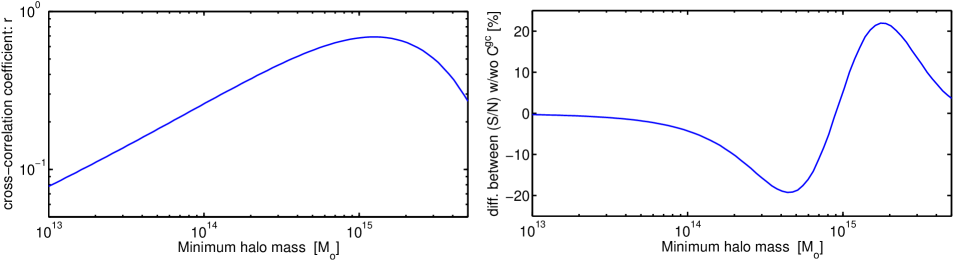
Figure 15: Left panel: Correlation coefficient $r$ between cluster counts and the lensing power spectrum for the simple toy model containing only the halo mass function and mass weighting. Right panel: Percentage difference in $S/N$ (to be compared with the lower panel of Fig. 7) for the simple toy model containing only the halo mass function and mass weighting.

The shape is remarkably similar to that for the full treatment, implying that this simple model containing the different weightings of the mass function captures the essence of the complementarity. The correlation peaks at around $10^{15}M_{\odot}$ and decreases at low minimum cluster masses. It makes sense that the cluster counts and lensing are correlated at high minimum cluster masses, because the mass weighting in the toy lensing power spectrum is similar to the mass cut in the cluster counts: they are both dominated by high mass clusters. They become less correlated at lower minimum masses because the cluster counts are dominated by low mass clusters that contribute less to the lensing power spectrum.

The size of the correlation is larger for this simple model than for the full treatment. This makes sense because the full model contains several ingredients that will reduce the correlation including: the contributions of the Gaussian errors and shot noise to the lensing power spectrum covariance (e.g., compare thick and thin lines in the lower panel of Fig. 5); halos at a range of redshifts which will be weighted differently by the lensing power spectra and cluster counts; and terms involving more than one halo at a time. However an even simpler toy model, in which all halos in the universe have the same mass, would make lensing power spectra and cluster counts 100 per cent correlated. We see that simply including the mass weighting $\propto m^{2}$ for the lensing power spectra stops a complete redundancy of information and starts to explain how these seemingly similar probes can be so complementary.

In this simple model we have only one data point from cluster counts $D^{c}$ and one data point from lensing $D^{g}$ (since we have only one redshift bin for each, and we are considering a single wavenumber $l$). Therefore we can write the signal-to-noise in terms of the correlation coefficient

$$\left(\frac{S}{N}\right)^{2}=\frac{1}{(1-r^{2})}\left(\frac{D^{g\,2}}{\bm{C}^{g}}+\frac{D^{c\,2}}{\bm{C}^{c}}-\frac{2D^{g}D^{c}}{\bm{C}^{gc}}r\right).$$ (81)

All the terms scale with ($\Omega_{\rm s}\chi^{2}\delta\chi$), the comoving volume of the redshift interval considered. We use a redshift slice at $z=0.3$ of thickness $0.1$ for illustration.

To reproduce the plot of percentage difference in $(S/N)$ we need to compare this to the $(S/N)$ when the covariance is not taken into account, found by setting $r=0$ in the above. The factor $1/(1-r^{2})$ is close to unity when the correlation coefficient $r$ is small, but when the correlation is strong ($r\sim 1$) it gets much larger. This causes the $(S/N)$ to be larger when the covariance is included than when it is not included and gives rise to the peak in the right hand panel of Fig. 15. The final term in the round brackets causes a decrease in $S/N$, relative to the case where no covariance is included. This is important especially when the correlation is small and the factor $1/(1-r^{2})$ is unimportant. This explains the dip in right hand panel of Fig. 15. In summary: the fact that Fig. 15 is qualitatively similar to the lower panel of Fig. 7 suggests that the peak and dip can be explained just in terms of the different mass weighting of cluster counts and the lensing power spectrum.

References

- (1) D. Spergel et al., Astrophys. J. Suppl. 665, 355 (2007).
- (2) S. Cole, et al., Mon. Not. Roy. Astr. Soc. 362, 505 (2005).
- (3) M. Tegmark, et al., Phys. Rev. D 74, 123507 (2006).
- (4) S. Weinberg, Mod. Rev. Phys. 61, 1 (1989).
- (5) B. Ratra and P. J. E. Peebles, Phys. Rev. D 37, 3406 (1988).
- (6) The Panoramic Survey Telescope & Rapid Response System (Pan-STARRS) http://pan-starrs.ifa.hawaii.edu
- (7) The Dark Energy Survey (DES) http://www.darkenergysurvey.org
- (8) Hyper Suprime-Cam Survey, S. Miyazaki, et al. SPIE 6269, 9 (2006).
- (9) The Large Synoptic Sky Survey (LSST) http://www.lsst.org
- (10) Wide Field Multi-Object Spectrograph (WFMOS), K. Glazebrook et al., astro-ph/0507457
- (11) The Dark UNiverse Explorer (DUNE) http://www.dune-mission.net/
- (12) The Supernova Acceleration Probe (SNAP) http://snap.lbl.gov/
- (13) M. Takada, E. Komatsu, T. Futamase, Phys. Rev. D 73, 083520 (2006).
- (14) A. Albrecht, et al. (Report on the Dark Energy Task Force), astro-ph/0609591
- (15) C. L. Sarazin, X-ray emission from clusters of galaxies, Cambridge University Press (1988)
- (16) P. B. Lilje, Astrophys. J. Lett. 33, 386 (1992).
- (17) N. A. Bahcall and R. Cen, Astrophys. J. Lett. 49, 407 (1993).
- (18) H. Hanami, Astrophys. J. 415, 42 (1993).
- (19) S. D. M. White, G. Efstathiou and C. S. Frenk, Mon. Not. Roy. Astr. Soc.262, 1023 (1993).
- (20) T. Kitayama and Y. Suto, Astrophys. J. 490, 557 (1997).
- (21) Z. Haiman, J. J. Mohr and G. P. Holder, Astrophys. J. 553, 545 (2000).
- (22) J. Weller, R. A. Battye and R. Kneissl, Phys. Rev. Lett. 88, 231301 (2001).
- (23) M. Lima and W. Hu, Phys. Rev. D 70, 043503 (2004).
- (24) S. Wang, J. Khoury, Z. Haiman, M. May, Phys. Rev. D 70, 123008 (2004).
- (25) L. Marian and G. M. Bernstein, Phys. Rev. D 73, 123525 (2006).
- (26) W. Hu, Phys. Rev. D 67, 081304 (2003).
- (27) S. Majumdar and J. J. Mohr, Astrophys. J. 613, 41 (2004).
- (28) W. Hu and Z. Haiman, Phys. Rev. D 68, 063004 (2003).
- (29) L. Van Waerbeke et al., A&A358, 30 (2000).
- (30) D. J. Bacon, A. R. Refregier, and R. S. Ellis, Mon. Not. Roy. Astr. Soc.318, 625 (2000).
- (31) D. M. Wittman, J. A. Tyson, D. Kirkman, I. Dell’Antonio, and G. Bernstein, Nature (London) 405, 143 (2000).
- (32) N. Kaiser, G. Wilson and G. A. Luppino, astro-ph/003338
- (33) M. Jarvis, B. Jain, G. Bernstein and D. Dolney, Astrophys. J. 644, 71 (2006).
- (34) H. Hoekstra et al, Astrophys. J. , 647, 116 (2006).
- (35) R. Massey et al (astro-ph/0701480)
- (36) C. Schimd et al, A&A, 463, 405 (2007).
- (37) W. Hu, Astrophys. J. Lett. 522, 21 (1999).
- (38) D. Huterer, Phys. Rev. D 65, 3001 (2002).
- (39) M. Takada and B. Jain, Mon. Not. Roy. Astr. Soc. 348, 897 (2004).
- (40) B. Koester et al., astro-ph/0701268
- (41) M. Gladders and H. Yee, ApJS 157, 1, (2005).
- (42) S. Miyazaki, T. Hamana et al., Astrophys. J. Lett. 580, 97 (2002).
- (43) D. Wittman, I. Dell’Antonio, J. Hughes, V. Margoniner, J.A. Tyson, J. Cohen and D. Norman, Astrophys. J. 643, 128 (2006).
- (44) S. Miyazaki, T. Hamana, R. S. Ellis, N. Kashikawa, R. J. Massey, J. Taylor, A. Refregier, astro-ph/0707.2249
- (45) W. Hu and M. White, Astrophys. J. 554, 67 (2001).
- (46) A. Cooray & W. Hu Astrophys. J. , 554 56 (2001).
- (47) M. Kilbinger and P. Schneider, A&A 442, 69 (2005).
- (48) M. Takada and B. Jain, in preparation (2007).
- (49) W. Fang and Z. Haiman, astro-ph/0612187 (2006).
- (50) S. Dodelson, Modern Cosmology, Academic Press, San Diego (2003).
- (51) M. Takada, Phys. Rev. D 74, 043505 (2006).
- (52) J. Carlstrom, G. Holder, E. Reese, Ann. Rev. Astron. Astrophys. 40, 643 (2002).
- (53) N. Kaiser and G. Squires, Astrophys. J. 404, 441 (1993).
- (54) T. Hamana, M. Takada and N. Yoshida, Mon. Not. Roy. Astr. Soc. 350, 893 (2004).
- (55) J. Navarro, C. Frenk, S. D. M. White, Astrophys. J. 490, 493 (1997).
- (56) M. Takada and B. Jain, Mon. Not. Roy. Astr. Soc. 340, 580 (2003).
- (57) R. J. Scherrer and E. Bertschinger, Astrophys. J. 381, 349 (1991).
- (58) R. Scoccimarro, R. Sheth, L. Hui, B. Jain, Astrophys. J. 546, 20 (2001).
- (59) M. Takada and B. Jain, Mon. Not. Roy. Astr. Soc. 344, 857 (2003).
- (60) A. Cooray, R. Sheth, Phys. Rept. 372, 1 (2002).
- (61) R. K. Sheth and G. Tormen, Mon. Not. Roy. Astr. Soc. 308, 119 (1999).
- (62) W. Press and P. Schechter, Astrophys. J. 187, 425 (1974).
- (63) W. Hu and A. V. Kravtsov, Astrophys. J. 584, 702 (2003).
- (64) E. V. Linder and A. Jenkins, Mon. Not. Roy. Astr. Soc. 346, 573 (2003).
- (65) M. White and L. Van Waerbeke, Astrophys. J. 575, 640 (2002).
- (66) Y. Mellier, Ann. Rev. Astron. Astrophys. 37, 127 (1999).
- (67) M. Bartelmann and P. Schneider, Phys. Rep. 340, 291 (2001).
- (68) P. Schneider, Gravitational Lensing: Strong, Weak and Micro, Lecture Notes of 33rd Saas-Fee Advanced Course, G. Meylan, P. Jetzer & P. North (eds.), Springer-Verlag: Berlin (2006).
- (69) F. Simpson and S. Bridle, Phys. Rev. D 71, 083501 (2005).
- (70) D. Limber, Astrophys. J. 119, 655 (1954).
- (71) J. Jain, A. Connolly and M. Takada, , JCAP 0703, 013 (2007).
- (72) W. Hu, Phys. Rev. D 62, 043007 (2000).
- (73) R. E. Smith, J. A. Peacock, et al., Mon. Not. Roy. Astr. Soc. 341, 1311 (2003).
- (74) D. Huterer and M. Takada, Astropart. Phys. 23, 369 (2005).
- (75) Z. Ma, Astrophys. J. 665, 887 (2007).
- (76) H. J. Mo and S. D. M. White, Mon. Not. Roy. Astr. Soc. 282, 347 (1996).
- (77) R. Scoccimarro, M. Zaldarriaga and L. Hui, Astrophys. J. 527, 1 (1999).
- (78) D. Eisenstein and W. Hu, Astrophys. J. 511, 5 (1999).
- (79) M. Chevallier and D. Polarski, Int. J. Mod. Phys. D10, 213 (2001).
- (80) E. Linder, Phys. Rev. Lett. 90, 091301 (2003).
- (81) D. Huterer, M. Takada, G. M. Bernstein, B. Jain, B., Mon. Not. Roy. Astr. Soc. 366, 101 (2006).
- (82) M. C. Neyrinck, I. Szapudi, C. R. Rimes, Mon. Not. Roy. Astr. Soc. 370, L66 (2006).
- (83) M. C. Neyrinck, I. Szapudi, Mon. Not. Roy. Astr. Soc. 375, L51 (2007).
- (84) R. A. Fisher, J. Roy. Stat. Soc. 98, 39 (1935).
- (85) M. Tegmark, A. N. Taylor and A. F. Heavens, Astrophys. J. 480, 22 (1997).
- (86) D. Eisenstein, W. Hu and M. Tegmark, Astrophys. J. 518, 2 (1999).
- (87) U. Seljak and M. Zaldarriaga, Astrophys. J. 469, 437 (1996).
- (88) L. Knox, Y.-S. Song and H. Zhang, Astrophys. J. 652, 857 (2006).
- (89) Z. Ma, W. Hu and D. Huterer, Astrophys. J. 636, 21 (2005).
- (90) E. Rozo, et al., astro-ph/0703571
- (91) H. Zhan, JCAP 0608, 008 (2006).
- (92) L. Bridle and L. King, astro-ph/0705.0166
- (93) R. Mandelbaum, C. M. Hirata, T. Broderick, U. Seljak, J. Brinkmann, Mon. Not. Roy. Astr. Soc. 370, 1008 (2006).
- (94) C. Hirata and U. Seljak, 2004, Phys. Rev. D 70, 063526 (2004).
- (95) W. Hu and B. Jain, Phys. Rev. D 70, 043009 (2004).
- (96) B. Jain and A. N. Taylor, Phys. Rev. Lett. 91, 141302 (2003).
- (97) D. Bacon, D. Goldberg, B. Rowe, A.N. Taylor, Mon. Not. Roy. Astr. Soc. 365, 414 (2006).
- (98) Y. Okura, T. Futamase and K. Umetsu, Astrophys. J. in press, astro-ph/0607288.
- (99) P.J. E. Peebles, A&A 32, 197 (1974).
- (100) J. McClelland and J. Silk, Astrophys. J. 216, 665 (1977).
- (101) P. J. E. Peebles, The Large-Scale Structure of the Universe, Princeton University Press, Princeton (1980).
- (102) F. Bernardeau, S. Colombi, E. Gaztanaga, R. Scoccimarro, Phys. Rept. 367, 1 (2002).