A new analysis of the Poincaré dodecahedral space model

Abstract

Context. The full three–year Wilkinson Microwave Anisotropy Probe results (hereafter WMAP3) reinforce the absence of large–angle correlations at scales greater than $60\degr$. The Poincaré dodecahedral space model, which may naturally explain such features, thus remains a plausible cosmological model, despite recent controversy about whether matched circle searches would or would not push the topology beyond the horizon.

Aims. We have used new eigenmode calculations of the dodecahedral space to predict the cosmic microwave background (CMB) temperature anisotropies in such a model, with an improved angular resolution.

Methods. We have simulated CMB maps and exhibited the expected self intersection of the last scattering surface along six pairs of circles. For a set of plausible cosmological parameters, we have derived the angular power spectrum of the CMB up to large wavenumbers.

Results. Comparison of the angular power spectrum with the WMAP3 observations leads to an optimal fit with the Poincaré dodecahedral space model, for a value $\Omega_{\mathrm{tot}}=1.018$ of the total energy density parameter.

1 Introduction

After lying dormant during the mid twentieth century, interest in cosmic topology re-awakened with the COBE satellite observations (Hinshaw et al. hin96 (1996)) followed by the first-year Wilkinson Microwave Anisotropy Probe observations (Bennett et al. WMAP1 (2003), hereafter WMAP1), which gave unexpected discrepancies with a $\Lambda$CDM model with infinite flat spatial sections (the so-called “concordance model”), including weak multipoles at $\ell$ = 2 and 3, and violations of statistical isotropy in the same multipoles (Schwarz et al. Schwarz (2004)). Among various possible explanations, it has been suggested that a spatially finite multi-connected universe may explain the weak large-angle correlations (Hinshaw et al. hin96 (1996); Spergel et al. WMAP1b (2003)). More precisely, when the spatial sections are taken to be the Poincaré dodecahedral space (PDS), the low-$\ell$ cosmic microwave background (CMB) multipoles fit well with the observational data (Luminet et al. Luminet (2003)), although it has been stated that the PDS model does not account for the violations of statistical anisotropy (Aurich et al. aurich07 (2007)). More generally, it was proved that the long-wavelength modes are relatively lowered in so-called “well-proportioned spaces” (Weeks et al. wp (2004)). Along with the PDS model, the well-proportioned spaces include roughly cubical flat tori and the binary tetrahedral and octahedral spaces. The power spectra for the octahedral and tetrahedral spaces have also been calculated and found to be consistent with the WMAP1 large-angle correlations (Aurich et al. ALS (2005)), although for rather high values of the density parameter $\Omega_{\mathrm{tot}}$, in conflict with the current observations.

The PDS model predicts pairs of matched antipodal circles as a definite signature (Cornish et al. CSS96 (1996)). Roukema (2000a ; 2000b ) was the first to apply the matched circle principle empirically to COBE data, whose poor angular resolution did not allow for a quantitative analysis. Next, different teams searched for such circles in the higher resolution WMAP1 data, using various statistical indicators and massive computer calculations. The team that first conceived the circle method obtained a negative result, which led them to reject the PDS model on a sub-horizon scale (Cornish et al. CSS04 (2004); Key et al. CSS06 (2007)). A second team, using a different analysis, found six pairs of matched circles distributed in a dodecahedral pattern, with angular sizes consistent with the PDS model, but they provided no statistical analysis so their claim remains unconvincing (Roukema et al. Roukema (2004)). A third team (Aurich et al. ALS (2005, 2006)) performed a more careful search and analysis and found that the signal was considerably degraded by the integrated Sachs-Wolfe (ISW) and Doppler contributions to the CMB temperature fluctuations (see Eq. 22 below). They concluded that the PDS model could be neither confirmed nor rejected by the circle search on presently available data. Then (then06 (2006)) also showed that even with foreground cleaned CMB maps, in which the most noisiest parts of the sky are masked, it is very hard to find matched circles. Thus, the topic remains controversial and the debate about the observational pertinence of the PDS remains open.

The recent release of the three-year WMAP results (Spergel et al. spergel07 (2007); Page et al. page07 (2007); Hinshaw et al. hinshaw07 (2007); Jarosik et al. jarosik07 (2007); hereafter WMAP3 papers) strengthens the evidence for weak large-angle correlations. The original WMAP1 analysis showed unusually weak CMB temperature correlations on angular scales greater than $60\degr$, at a confidence level of 99.85$\%$ (Spergel et al. WMAP1b (2003)). Still looking at scales greater than $60\degr$, an independent analysis finds the correlations to be weak at the 99.91$\%$ level for the WMAP1 data but then at the 99.97$\%$ level for the WMAP3 data (Copi et al. Copi06 (2006)), in both cases for the cut sky (which excludes local contamination from the Milky way). This strengthened evidence for weak large-angle correlations motivates continued interest in the PDS and related finite universe models.

A multi-connected space is the quotient $E=X/\Gamma$ of a simply connected space $X$ (the universal cover of $E$) under the action of a group $\Gamma$ of symmetries of $E$ (the holonomy group). For $E$ to be a manifold (rather than an orbifold or something more complicated still), the holonomy group $X$ must be discrete and fixed point free (see, e.g., Lachièze-Rey & Luminet lalu (1995)). The universal cover $X$ corresponds to a homogeneous spatial section of a standard Friedmann-Lemaître spacetime. In the case of the PDS, the universal cover is the three-sphere $\mathcal{S}^{3}$, and the finite holonomy group $\Gamma$ is generated by two elements, represented by two special orthogonal matrices.

This paper evaluates further the predictions of a PDS cosmological model and compares them with new CMB observations. This requires knowing the eigenmodes of the Laplacian on the PDS, i.e., the solution of its eigenvalue Helmoltz equation. Up until recently, only numerical solutions were available, and for the first modes only (corresponding to low wavenumbers $k$). For instance, the original calculations were purely numerical, and only up to $k=24$ (Luminet et al. Luminet (2003)). Later work extended the calculation to $k=230$ (Aurich et al. ALS (2005)). The present work is based on new analytical calculations of the eigenmodes of the PDS (Lachièze-Rey & Caillerie SCMLR (2005)), which are consistent with Bellon’s recent work (Bellon06 (2006)). They allowed us to compute modes for very high values of $k$, much beyond $k=230$. However, storage capacity limited the results presented in this article to $k=230$ as the number of modes goes as $k_{\mathrm{max}}^{3}$, because a mode $k$ is defined by the $(k+1)^{2}$ coefficients of its projection onto the modes of $\mathcal{S}^{3}$. If the aim is to calculate the power spectrum only (without simulating temperature maps), we can go further, up to $k=3\,000$, using a theorem of Gundermann (Gun (2005)), which was also conjectured independently by Aurich et al. (ALS_conj (2005)).

The eigenmodes of the multi-connected space $E$ lift to $\Gamma$-invariant modes of the universal cover $X$. Conversely, each $\Gamma$-invariant mode of $X$ projects down to a mode of $E$. Thus, we may safely visualize – and compute – the modes of $E$ as the $\Gamma$-invariant modes of $X$. They are the solutions $\psi$ of the Helmholtz equation:

$$\Delta_{X}\psi=\lambda_{k}\psi$$ (1)

where $\Delta_{X}$ is the Laplacian on $X$ and $\lambda_{k}$ is the eigenvalue associated to the integer wavenumber $k$. The invariance condition under $\Gamma$ reads

$$\psi(g(x))=\psi(x)$$ (2)

for all symmetries $g\in\Gamma$ and all points $x\in X$. It follows that each eigenvalue for a multi-connected space $E$ is also an eigenvalue for the universal cover $X$. When $X=S^{3}$, the eigenvalues take the form $\lambda_{k}=-k(k+2)$, indexed by integer wavenumbers $k\in\mathbb{N}$, with multiplicity $(k+1)^{2}$. The eigenvalues of the PDS form a subset of this set, given explicitly in Ikeda (Ikeda (1995)).

Given a model for gravitational instabilities, the statistical distribution of the CMB temperature fluctuations in the PDS model depends on the PDS’s eigenmodes. Applying the method of Lachièze-Rey & Caillerie (SCMLR (2005)), we construct the modes up to wavenumber $k_{\mathrm{max}}=230$. From them, we calculate the implied realizations of the CMB temperature. This lets us reach a resolution in the temperature fluctuations corresponding to the (curvature dependent) angular wavenumber $\ell_{\mathrm{max}}\sim k_{\mathrm{max}}\,\sqrt{\Omega_{\mathrm{tot}}-1}\sim 30$.

In Sect. 3, we show typical maps corresponding to realizations with angular resolution $\theta\sim 6\degr$. In these maps, we exhibit the expected presence of matched “circles in the sky” (Cornish et al. CSS98 (1998)).

From the realizations of the temperature distributions, we have generated a statistical set of realizations of the eigenmodes distribution. This allowed us to estimate expectation values and statistics for the characteristics of the CMB temperature distributions, in particular for the angular power spectrum coefficients $C_{\ell}$, up to the limit $\ell_{\mathrm{max}}$.

For the modes with lowest values of $\ell$ (up to 24), we confirm the previous calculations of Luminet et al. (Luminet (2003)). We extend them over a wider range of the spectrum and compare them with the WMAP3 data.

2 Eigenmodes of the Laplacian

We recall briefly the main results obtained in Lachièze-Rey & Caillerie (SCMLR (2005)), summarizing the key elements and including practical details concerning the eigenmodes of the PDS, i.e., the solutions of Eqs. (1) and (2) for the PDS.

The solutions of the Helmholz equation (1) for the 3-sphere $S^{3}$ form a vector space $\mathcal{V}$, which is the direct sum of subspaces

$$\mathcal{V}=\bigoplus_{k=0}^{\infty}\mathcal{V}_{k}$$ (3)

where $\mathcal{V}_{k}$ denotes the space of eigenmodes of $\mathcal{S}^{3}$ with eigenvalue $\lambda_{k}=-k(k+2)$. Similarly, the vector space of eigenmodes of the PDS splits as the direct sum

$$\mathcal{V}^{\textrm{{\tiny PDS}}}=\bigoplus_{k=0}^{\infty}\mathcal{V}_{k}^{\textrm{{\tiny PDS}}}.$$ (4)

Each $\mathcal{V}_{k}^{\textrm{{\tiny PDS}}}$ is a (possibly empty) subspace of the corresponding $\mathcal{V}_{k}$. The dimension of $\mathcal{V}_{k}^{\textrm{{\tiny PDS}}}$ is the multiplicity of the eigenvalue $\lambda_{k}$ for the PDS, which is always an integer multiple of $k+1$ and is non-zero only if $k$ is even. Ikeda (Ikeda (1995)) has calculated the multiplicities explicitly.

Thanks to the splitting (4), we will compute the eigenmodes on each $\mathcal{V}_{k}^{\textrm{{\tiny PDS}}}$ separately. For convenience, we will express the modes of $\mathcal{V}_{k}^{\textrm{{\tiny PDS}}}$ relative to the basis of $\mathcal{V}_{k}$.

First, we consider the parabolic basis of $\mathcal{V}_{k}$, which was first introduced in Bander & Itzykson (Bander (1966)) by group theoretical arguments. It corresponds to the following set of functions $T_{k;m_{1},m_{2}}$, defined for $k,m_{1},m_{2}\in\mathbb{N}$ and $-k/2\leq(m_{1},m_{2})\leq k/2$ by:

$$\begin{array}[]{c c c}\mathcal{S}^{3}&\longrightarrow&\mathbb{C}\\ (\chi,\theta,\phi)&\longmapsto&\alpha(\cos\chi\,e^{i\theta})^{l}(\sin\chi\,e^{i\phi})^{m}P_{d}^{m,l}(\cos 2\chi)\\ \end{array}$$ (5)

where $l:=m_{1}+m_{2}$, $m:=m_{2}-m_{1}$, $d=k/2-m_{2}$ and the coefficient

$$\alpha=\sqrt{\frac{k+1}{2\pi^{2}}}\sqrt{\frac{(k/2+m_{2})!(k/2-m_{2})!}{(k/2+m_{1})!(k/2-m_{1})!}}$$

is computed from normalization requirements. As $\mathbf{T}\equiv\{T_{k;m_{1},m_{2}}\}$ is a basis of $\mathcal{V}^{k}$, it generates $\mathcal{V}^{k}_{X}$, so each solution of (1) for the PDS can be decomposed on this set as:

$$\psi^{\textrm{{\tiny PDS}}}_{k}=\sum_{m_{1},m_{2}}f_{k;m_{1},m_{2}}\leavevmode\nobreak\ T_{k;m_{1},m_{2}}$$ (6)

where the $f_{k;m_{1},m_{2}}$ are complex numbers.

In order to be an eigenmode of the PDS, $\psi^{\textrm{{\tiny PDS}}}_{k}$ has to be invariant under $\Gamma$, the holonomy group of the PDS. To be so, it is sufficient that it be invariant under two generators, which we denote $g_{1}$ and $g_{2}$:

$$\psi^{\textrm{{\tiny PDS}}}_{k}(x)=\psi^{\textrm{{\tiny PDS}}}_{k}(g_{1}(x))\quad\textrm{and}\quad\psi^{\textrm{{\tiny PDS}}}_{k}(x)=\psi^{\textrm{{\tiny PDS}}}_{k}(g_{2}(x))$$ (7)

for all $x\in S^{3}$, or equivalently

$$R_{g_{1}}\psi^{\textrm{{\tiny PDS}}}_{k}=\psi^{\textrm{{\tiny PDS}}}_{k}\quad\textrm{and}\quad R_{g_{2}}\psi^{\textrm{{\tiny PDS}}}_{k}=\psi^{\textrm{{\tiny PDS}}}_{k}$$ (8)

where the operator $R_{g}$ expresses the natural left action of the $\mathrm{SO(4)}$ rotation $g$ defined as $(R_{g}\psi)(x)\equiv\psi(g^{-1}x)$.

To solve this system of equations, taking advantage of their nice properties under rotations on the sphere, we introduced the Wigner D-functions. This set of functions naturally acts on the Lie group $\mathrm{SO(3)}$ via the following action:

$$\begin{array}[]{r c c c}D^{j}_{m_{1},m_{2}}:&\mathrm{SO(3)}&\longrightarrow&\mathbb{C}\\ &g&\longmapsto&<j,m_{1}|R_{g}|j,m_{2}>.\\ \end{array}$$ (9)

The vectors $\mid jm>$, $-j\leq m\leq j$, form an orthonormal basis for $\mathcal{H}^{j}$, the $2j+1$ dimensional irreducible representation of $\mathrm{SU(2)}$. When $j$ is integer, this is also an irreducible unitary representation of $\mathrm{SO(3)}$, and the $\mid jm>$ can be taken as the usual spherical harmonics $Y_{jm}$. This implies

$$R_{g}Y_{jm}=\sum_{m^{\prime}=-j}^{j}{\cal D}_{m^{\prime}m}^{j}(g^{-1})\leavevmode\nobreak\ Y_{jm^{\prime}}.$$ (10)

In Lachièze-Rey & Caillerie (SCMLR (2005)), we also derived a useful identity describing the action of these functions on the product of two elements of $\mathrm{SO(3)}$,

$$D^{j}_{m_{1},m_{2}}(gh)=\sum_{m}D^{j}_{m,m_{2}}(g)\leavevmode\nobreak\ D^{j}_{m_{1},m}(h),$$ (11)

which is just the resolution of the identity in their definition (9).

The isometry between $\mathcal{S}^{3}$ and $\mathrm{SU(2)}$, as manifolds, allows us to link these functions with those of the parabolic basis. Any point of $\mathcal{S}^{3}$ is identified to an element of $\mathrm{SU(2)}$ by the following relation:

$$\begin{array}[]{c c c}\mathcal{S}^{3}&\longrightarrow&\mathrm{SU(2)}\\ x\equiv(\chi,\theta,\phi)&\longmapsto&u_{x}\equiv\left(\begin{array}[]{c c}\cos\chi\leavevmode\nobreak\ e^{i\theta}&i\leavevmode\nobreak\ \sin\chi\leavevmode\nobreak\ e^{i\phi}\\ i\leavevmode\nobreak\ \sin\chi\leavevmode\nobreak\ e^{-i\phi}&\cos\chi\leavevmode\nobreak\ e^{-i\theta}\\ \end{array}\right).\\ \end{array}$$ (12)

Note that one finds other phase choices for this identification in the literature.

On the other hand, there is a group isomorphism between $\mathrm{SU(2)}$/$\mathbb{Z}_{2}$ and $\mathrm{SO(3)}$, where $\mathbb{Z}_{2}$ refers to the multiplicative group $\{+id,-id\}$. Thus, each element $u$ of $\mathrm{SU(2)}$ defines a rotation $g_{u}$ in $\mathrm{SO(3)}$. In practice, a rotation of $\mathrm{SO(3)}$ is parameterized by its Euler angles $\alpha$, $\beta$, $\gamma$. Taking into account the identification above, the correspondence takes the form:

$$\begin{array}[]{c c c}\mathrm{SU(2)}{}&\longrightarrow&\mathrm{SO(3)}\\ u=(\chi,\theta,\phi)&\longmapsto&g_{u}=(\alpha,\beta,\gamma),\\ \end{array}$$ (13)

with

$$\chi=\frac{\beta}{2}\qquad\theta=\frac{\alpha+\gamma}{2}\qquad\phi=\frac{\alpha-\gamma}{2}.$$ (14)

This lets us lift the Wigner D-functions from $\mathrm{SO(3)}$  to $\mathrm{SU(2)}$ or, equivalently, to $\mathcal{S}^{3}$. Their explicit expression (see for instance Edmonds Edmonds (1960)) shows the identification, up to a constant, with the previous functions $T_{k;m_{1},m_{2}}$:

$$D^{k/2}_{m_{2},m_{1}}(u_{x})\equiv\sqrt{\frac{2\pi^{2}}{k+1}}\leavevmode\nobreak\ T_{k;m_{1},m_{2}}(u),$$ (15)

with $-k/2\leq m_{1},m_{2}\leq k/2$.

We can now write Eq. (7) explicitly, by expanding modes on the parabolic basis. This gives, for any $x$ in $\mathcal{S}^{3}$,

$$\sum_{m_{1},m_{2}}f_{k;m_{1},m_{2}}T_{k;m_{1},m_{2}}(x)=\sum_{m_{1},m_{2}}f_{k;m_{1},m_{2}}\leavevmode\nobreak\ T_{k;m_{1},m_{2}}(g^{-1}x)$$ (16)

where $g$ is one of the two generators ($g_{1}$ or $g_{2}$) of the PDS (or, if desired, of some other spherical space). Using property (11), we obtain a simple relation between the coefficients of the eigenmodes:

$$f_{k;m_{1},m_{2}}=\sum_{m}f_{k;m_{1},m}\leavevmode\nobreak\ D^{k/2}_{m,m_{2}}(g^{-1}).$$ (17)

Note that this equation is independent of the index $m_{1}$, so we can further split each vector subspace as a direct sum

$$\mathcal{V}_{k}^{\textrm{{\tiny PDS}}}=\bigoplus\mathcal{V}_{k,m_{1}}^{\textrm{{\tiny PDS}}}.$$ (18)

More practically, this corresponds to writing the eigenmode $f_{k;m_{1},m_{2}}$ as

$$f_{k;m_{1},m_{2}}=f_{km_{2}}\leavevmode\nobreak\ \delta_{m_{0}m_{1}},$$ (19)

where $m_{0}$ is some arbitrary integer between $-k/2$ and $k/2$. This implies that the multiplicity of an eigenmode of a spherical space is proportional to $k+1$. Thus, we may rewrite Eq. (17) as an eigenvalue equation

$$D_{k,g}F_{k}=F_{k}$$ (20)

where $F_{k}$ is the vector with coordinates $f_{km_{2}}$ and $D_{k,g}$ is the matrix whose general term is $D^{k/2}_{m,m_{2}}(g^{-1})$. This gives a system of two eigenvalue equations to be solved simultaneously. In Lachièze-Rey & Caillerie (SCMLR (2005)), we have shown that when we choose a basis of the three-sphere where one generator, say $g_{1}$, is diagonal (which is always possible), this imposes the condition

$$m_{2}=0\pmod{n}$$ (21)

where the integer $n$ equals $5$ in the case of the PDS. In this case, finding the eigenmodes of the Laplacian corresponds to finding a solution of (20) for $g=g_{2}$ and where we consider only indices $m_{2}$ satisfying the condition (21).

3 Temperature maps

We now restrict our study to cosmological models whose spatial section is a PDS, and to values of $\Omega_{\mathrm{tot}}$ in the range favored by the WMAP1 and WMAP3 observations, namely $\Omega_{\mathrm{tot}}=1.02\pm 0.02$.

3.1 Maps

Matter fluctuations at recombination are assumed to follow a Gaussian random distribution with a Harrison-Zel’dovich power spectrum with $P(k)\propto k^{1}$. Thus, a realization is given by a Gaussian random distribution of the modes calculated in the previous section, constrained to have the desired power spectrum law. However, as first emphasized by Roukema (2000a ), the power spectrum approaching the injectivity diameter and the out-diameter of the fundamental domain may well be different from the theoretical $k^{1}$ expectation, since these scales represent the physical size of the whole universe, and the observational arguments for a $k^{1}$ spectrum at these scales are only valid by assuming simple connectedness. This can be considered as a caveat for the interpretation of the following results.

Such a distribution of matter fluctuations generates a temperature distribution on the CMB that results from different physical effects. If we subtract foreground contamination, it will mainly be generated by the ordinary Sachs-Wolfe (OSW) effect at large scales, resulting from the the energy exchanges between the CMB photons and the time-varying gravitational fields on the last scattering surface (LSS). At smaller scales, Doppler oscillations, which arise from the acoustic motion of the baryon-photon fluid, are also important, as well as the OSW effect. The ISW effect, important at larger scales, has the same physical origin as the OSW effect but is integrated along the line of sight rather than on the LSS. This is summarized in the Sachs-Wolfe formula, which gives the temperature fluctuations in a given direction $\hat{n}$ as

$$\frac{\delta T}{T}(\hat{n})=\left(\frac{1}{4}\frac{\delta\rho}{\rho}+\Phi\right)(\eta_{\mathrm{LSS}})-\hat{n}.\mathbf{v}_{e}(\eta_{\mathrm{LSS}})+\int_{\eta_{\mathrm{LSS}}}^{\eta_{0}}(\dot{\Phi}+\dot{\Psi})\,\mathrm{d}\eta$$ (22)

where the quantities $\Phi$ and $\Psi$ are the usual Bardeen potentials, and ${\bf v}_{e}$ is the velocity within the electron fluid; overdots denote time derivatives. The first terms represent the Sachs-Wolfe and Doppler contributions, evaluated at the LSS. The last term is the ISW effect. This formula is independent of the spatial topology, and is valid in the limit of an infinitely thin LSS, neglecting reionization.

The temperature distribution is calculated with a CMBFast–like software developed by one of us, under the form of temperature fluctuation maps at the LSS. One such realization is shown in Fig. 1, where the modes up to $k=230$ give an angular resolution of about $6\degr$ (i.e. roughly comparable to the resolution of COBE map), thus without as fine details as in WMAP data. However, this suffices for a study of topological effects, which are dominant at larger scales.

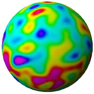
Figure 1: Temperature map for a Poincaré dodecahedral space with $\Omega_{\mathrm{tot}}=1.02$, $\Omega_{\mathrm{mat}}=0.27$ and $h=0.70$ (using modes up to $k=230$ for a resolution of $6\degr$).

Such maps are the starting point for topological analysis: firstly, for noise analysis in the search for matched circle pairs, as described in Sect. 3.2; secondly, through their decompositions into spherical harmonics, which predict the power spectrum, as described in Sect. 4. In these two ways, the maps allow direct comparison between observational data and theory.

3.2 Circles in the sky

A multi-connected space can be seen as a cell (called the fundamental domain), copies of which tile the universal cover. If the radius of the LSS is greater than the typical radius of the cell, the LSS wraps all the way around the universe and intersects itself along circles. Each circle of self-intersection appears to the observer as two different circles on different parts of the sky, but with the same OSW components in their temperature fluctuations, because the two different circles on the sky are really the same circle in space. If the LSS is not too much bigger than the fundamental cell, each circle pair lies in the planes of two matching faces of the fundamental cell. Figure 2 shows the intersection of the various translates of the LSS in the universal cover, as seen by an observer sitting inside one of them.

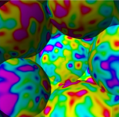
Figure 2: The last scattering surface seen from outside in the universal covering space of the Poincaré dodecahedral space with $\Omega_{\mathrm{tot}}=1.02$, $\Omega_{\mathrm{mat}}=0.27$ and $h=0.70$ (using modes up to $k=230$ for a resolution of $6\degr$). Since the volume of the physical space is about 80% of the volume of the last scattering surface, the latter intersects itself along six pairs of matching circles.

These circles are generated by a pure Sachs-Wolfe effect; in reality additional contributions to the CMB temperature fluctuations (Doppler and ISW effects) blur the topological signal. Two teams have carefully analyzed the blurring in the case of the Poincaré dodecahedral space: one team finds it strong enough to hide matching circles (Aurich et al. ALS (2005, 2006)), while the other team reaches the opposite conclusion (Cornish et al. CSS04 (2004); Shapiro Key et al. CSS06 (2007)). By contrast, in the case of a small 3-torus universe, everyone agrees that blurring could not hide circles. The blurring’s effectiveness varies by topology, because the relative strengths of the various effects (OSW, ISW, Doppler) depend on the modes of the underlying space.

4 Power spectrum

Like any function defined on the sphere, the CMB temperature fluctuations can be decomposed into spherical harmonics

$$\frac{\delta T}{T}(\hat{n})=\sum_{l=0}^{+\infty}\sum_{m=-l}^{l}a_{lm}\leavevmode\nobreak\ Y_{lm}(\hat{n})$$ (23)

where the unit vector $\hat{n}\in S^{2}$ represents a point on the sky.

For a statistically homogeneous and isotropic distribution of matter in the universe, the power spectrum

$$C_{l}:=\frac{1}{2l+1}\sum_{m=-l}^{l}<a_{lm}a_{lm}^{*}>.$$ (24)

contains all relevant information about the temperature fluctuations. Such a power spectrum has been calculated for the CMB temperature fluctuations as measured by WMAP. We compare it here with the predictions of our model.

From our realizations of the predicted temperature maps, we have calculated power spectra. Assuming a present day matter density $\Omega_{\mathrm{mat}}=0.27$ and a reduced Hubble parameter $h=0.70$ (Spergel et al., spergel07 (2007)), we have varied $\Omega_{\mathrm{tot}}$ within the range 1.015–1.025, where we get low-$l$ power compatible with WMAP3 data. For illustrative purposes, Fig. 3 shows our estimated spectra for the PDS, using three values of $\Omega_{\mathrm{tot}}$ within the above range, compared with the WMAP3 data taken from Fig. 2 of Spergel et al. (spergel07 (2007)). We have normalized the curves by insisting that they approach the concordance model curve for high $\ell$, because topology is significant only for low $\ell$. We can see that the PDS model agrees well with observations for all three values of $\Omega_{\mathrm{tot}}$, up to the cutoff $\ell_{\mathrm{max}}\sim k_{\mathrm{max}}\sqrt{\Omega_{\mathrm{tot}}-1}$. Since our numerical computations go only to wavenumber $k_{\mathrm{max}}\sim 230$, the resulting power spectrum is reliable only up to $\ell\sim 25-30$, depending on $\Omega_{\mathrm{tot}}$. The oscillatory pattern in the $C_{l}$ is a prediction of the Poincaré dodecahedral space model due to multiplicities by which the vibrational modes are weighted in the mode sum. The effect is significant only for the low vibrational modes; it is washed out at sufficiently large $l$ ($l\gtrsim 30$) so that the asymptotic behaviour of the power spectrum recovers the curve for the simply connected ${\cal S}^{3}$.

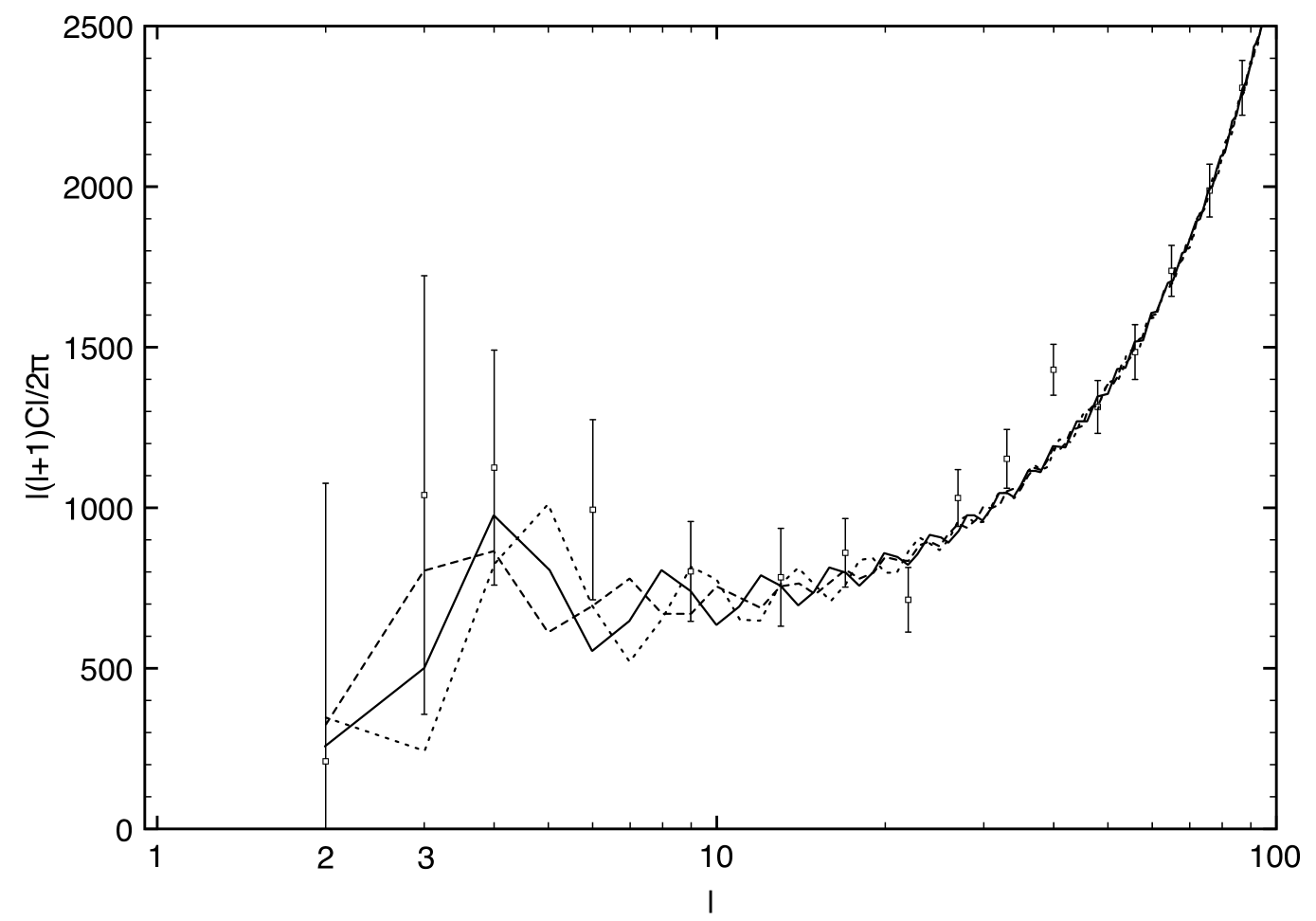
Figure 3: Comparative power spectra (in $\mu\mathrm{K}^{2}$) as a function of the multipole $\ell$ for WMAP3 (errorbars) and PDS for three values of $\Omega_{\mathrm{tot}}$ ($\Omega_{\mathrm{tot}}=1.015$ for the dashed curve, $\Omega_{\mathrm{tot}}=1.02$ for the solid curve and $\Omega_{\mathrm{tot}}=1.025$ for the dotted curve), assuming $\Omega_{\mathrm{mat}}=0.27$ and $h=0.70$. Here we calculate the modes up to $k=3000$ using the conjecture of Aurich et al. (ALS_conj (2005)) proved by Gunderman (Gun (2005)).

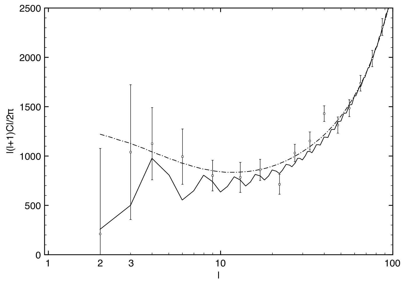
Figure 4: Comparative power spectra (in $\mu\mathrm{K}^{2}$) as a function of the multipole $\ell$ for WMAP3 (errorbars), “concordance model” (dot-dashed curve) and PDS (solid curve) for $\Omega_{\mathrm{tot}}=1.018$, $\Omega_{\mathrm{mat}}=0.27$ and $h=0.70$.

Figure 4 shows the optimal fit at $\Omega_{\mathrm{tot}}=1.018$ for which the quadrupole suppression is maximal, a value perfectly consistent with the WMAP team reported $\Omega_{\mathrm{tot}}=1.02\pm 0.02$. In order to compare the predictions of simply connected and multi-connected topologies, we also compare our best fit PDS spectrum with the standard best fit “concordance model” spectrum.

5 Conclusion

Recent analytical eigenmode calculations for the Poincaré dodecahedral space allowed us to simulate CMB temperature fluctuation maps more accurately. We confirmed the correctness of the maps by verifying the presence of the expected circles-in-the-sky in the OSW-only maps.

Using a random set of Gaussian realizations of the matter fluctuations, we have calculated the predicted power spectrum of the CMB temperature fluctuations and the two-point temperature correlation function. Our results for the lowest modes confirm the numerical estimates of Luminet et al. (Luminet (2003)), while use of higher PDS modes let us estimate the multipoles up to $\ell\sim 30$. We have obtained an excellent fit with the WMAP data, implying that the PDS cosmological model remains a good candidate for explaining the angular spectrum, even though the negative results of matching circle searches remain a topic of debate (Key et al. CSS06 (2007); Aurich et al. ALS1 (2006); Then then06 (2006)).

Clearly the power spectrum alone cannot confirm a multiconnected cosmological model. Although the PDS model fits the WMAP3 power spectrum better than the standard flat infinite model does, alternative explanations may still be found, the simplest one being an intrinsically non-scale invariant spectrum. Thus, one must find complementary checks of the topological hypothesis. The off-diagonal terms of the correlation matrix provide one possibility. Unfortunately, they are not easy to derive and are difficult to interpret statistically. On the other hand, polarization effects provide an additional tool for investigating space topology (Riazuelo et al. pol (2006)).

- (1) Aurich R., Lustig S., Steiner F. and Then H., 2007, Class.Quant.Grav. 24, 1879-1894.
- (2) Aurich R., Lustig S. & Steiner F., 2006, MNRAS 369, 240-248.
- (3) Aurich R., Lustig S. & Steiner F., 2005a, Class. Quant. Grav. 22, 3443.
- (4) Aurich R., Lustig S. & Steiner F., 2005b, Class. Quant. Grav. 22, 2061.
- (5) Bander M. & Itzykson C., 1996, Rev. Mod. Phys. 18, 2.
- (6) Bellon M., 2006, Class. Quant. Grav. 23, 7029-7043.
- (7) Bennett C. L. et al., 2003, ApJS 148, 1.
- (8) Copi C. J., Huterer D., Schwarz D.J. & Starkman G. D., 2007, Phys. Rev. D 75, 023507.
- (9) Cornish N. J., Spergel D. N. & Starkman G. D., 1996, gr-qc/9602039.
- (10) Cornish N. J., Spergel D. N. & Starkman G. D., 1998, Class. Quant. Grav. 15, 2657.
- (11) Cornish N. J., Spergel D. N., Starkman G. D. & Komatsu E., 2004, PRL 92, 201302.
- (12) Edmonds A. R., 1960, Angular momentum on quantum mechanics, Princeton University Press.
- (13) Gundermann J., 2005, astro-ph/0503014.
- (14) Hinshaw G. et al., 1996, ApJL 464, L17.
- (15) Hinshaw G. et al., 2007, ApJS 170, 288.
- (16) Ikeda A., 1995, Kodai Math. J. 18, 57-67.
- (17) Jarosik N. et al., 2007, ApJS 170, 263.
- (18) Key S. J., Cornish N. J., Spergel D. N. & Starkman G. D., 2007, Phys. Rev. D 75, 084034.
- (19) Lachièze-Rey M. and Luminet J.-P., 1995, Phys. Rep. 254, 135.
- (20) Lachièze-Rey M. and Caillerie S., 2005, Class. Quant. Grav. 22, 695.
- (21) Luminet J.-P., Weeks J., Riazuelo A., Lehoucq R. & Uzan J.-P., 2003, Nature 425, 593.
- (22) Page L. et al., 2007, ApJS 170, 335.
- (23) Riazuelo A., Caillerie S., Lachièze-Rey M., Lehoucq R. & Luminet J.-P., astro-ph/0601433.
- (24) Roukema B. F., 2000a, MNRAS 312, 712.
- (25) Roukema B. F., 2000b, Class. Quant. Grav. 17, 3951.
- (26) Roukema B. F., Lew B., Cechowska M., Marecki A. & Bajtlik S., 2004, A&A 423, 821.
- (27) Schwarz D. J. et al., 2004, PRL 93, 221301.
- (28) Spergel D. N. et al., 2003, ApJS 148, 175.
- (29) Spergel D. N. et al., 2007, ApJS 170, 377.
- (30) Then H., 2006, MNRAS 373, 139.
- (31) Weeks J., Luminet J.-P., Riazuelo A. & Lehoucq R., 2004, MNRAS 352, 258.