J1128+592: a highly variable IDV source

Abstract

Short time-scale radio variations of compact extragalactic radio quasars and blazars known as IntraDay Variability (IDV) can be explained in at least some sources as a propagation effect; the variations are interpreted as scintillation of radio waves in the turbulent interstellar medium of the Milky Way. One of the most convincing observational arguments in favor of a propagation-induced variability scenario is the observed annual modulation in the characteristic time scale of the variation due to the Earth’s orbital motion. So far there are only two sources known with a well-constrained seasonal cycle. Annual modulation has been proposed for a few other less well-documented objects. However, for some other IDV sources source-intrinsic structural variations which cause drastic changes in the variability time scale were also suggested. J1128+592 is a recently discovered, highly variable IDV source. Previous, densely time-sampled flux-density measurements with the Effelsberg 100-m radio telescope (Germany) and the Urumqi 25-m radio telescope (China), strongly indicate an annual modulation of the time scale. The most recent 4 observations in 2006/7, however, do not fit well to the annual modulation model proposed before. In this paper, we investigate a possible explanation of this discrepancy.

1 Introduction

Short time-scale (few hours to few days long) variations of the radio flux density in flat spectrum radio-loud quasars and blazars were discovered in the mid-eighties (Witzel et al. 1986; Heeschen et al. 1987). The phenomenon was named IntraDay Variability (IDV). If interpreted as being source intrinsic, the short time scale of the variations would imply – through the light travel time argument – micro-arcsecond-scale sizes of the emitting regions, which would result in excessively large apparent brightness temperatures. The calculated variability brightness temperatures obtained are typically in the range of $10^{16}\text{\,K to }10^{21}$ K, which is far in excess of the inverse-Compton limit of $\sim 10^{12}$ K (Kellermann & Pauliny-Toth 1969). Thus, theories which explain IDV with variations intrinsic to the quasar, require excessively large Doppler boosting factors ($\delta$ $\gg$ $50$) or special source geometries (such as non-spherical relativistic emission models,
e.g. Qian et al. 1996a, b, 1991; Spada et al. 1999) or coherent and collective plasma emission (Benford 1992; Lesch & Pohl 1992) to avoid the inverse-Compton catastrophe.

An alternative theory explains IDV as a propagation effect. In this source-extrinsic interpretation, IDV is caused by interstellar scintillation (ISS) of radio waves in the turbulent plasma of the Milky Way. One of the most convincing arguments in favor of an extrinsic explanation of IDV is the so called annual modulation of the IDV time scale. The characteristic variability time scale is inversely proportional to the relative velocity between the observer and the scattering medium. The observer’s velocity (and so the relative velocity vector between the observer and scattering medium) undergoes a systematic annual modulation as the Earth orbits around the Sun. This annual velocity variation then is observed as an annual change in the variability time scale. Such seasonal cycles are seen in two IDV sources: J1819+3845 (Dennett-Thorpe & de Bruyn 2003) and PKS1257-326 (Bignall et al. 2003). In a few other IDV sources, such as PKS1519-273 (Jauncey et al. 2003),
B0917+624 (Rickett et al. 2001; Jauncey & Macquart 2001) PKS0405-385 (Kedziora-Chudczer 2006) and B0954+658 (Fuhrmann priv. com.), different characteristic variability time scales were measured at different observing epochs, however systematic seasonal variations, as expected from the annual modulation model, were either not seen or could not be unambiguously identified. The IDV sources
B0917+624 (Fuhrmann et al. 2002) and PKS0405-385 seem to display the so called episodic IDV (e.g.
Kedziora-Chudczer 2006), where pronounced variability is observed for months or even years and then temporarily stops and the IDV ceases. This variability behaviour may be due to changes in the intrinsic source structure (expansion of the scintillating component) or changes in the scattering plasma (Kraus et al. 1999; Krichbaum et al. 2002; Bernhart et al. 2006; Kedziora-Chudczer 2006).

If IDV is caused by ISS, it is possible to predict the frequency dependence of the variability amplitude, which above a transition frequency from strong to weak scintillation is expected to be less pronounced towards higher observing frequencies. However, observations of several IDV sources (most notably S50716+71, Kraus et al. 2003; Agudo et al. 2006; Ostorero et al. 2006) do not show such a frequency dependence and show variability amplitudes which increase with frequency. Krichbaum et al. (2002) suggested that a source-intrinsic contribution may cause the discrepancy between the observed and the expected frequency dependence.

For a better understanding of the IDV phenomenon, a clear distinction between ISS induced propagation effects and a source-intrinsic origin of the variability is important. Here, we present the variability characteristics of the recently discovered highly variable IDV source J1128+592 and discuss the possible mixture of ISS-induced and source-intrinsic variability.

2 Observations

J1128+592 was observed with the Max-Planck-Institut für Radioastronomie (MPIfR) 100-m Effelsberg radio telescope (at 2.70, 4.85 and 10.45 GHz) and with the Urumqi radio telescope (at 4.85 GHz) in so far 15 observing sessions, each lasting several days. The results of the first ten epochs of observations are already published in Gabányi et al. (2007).

The low-noise 4.85 GHz receiver, a new receiver backend and new telescope driving software for the Urumqi telescope were provided by the MPIfR. A detailed technical description of the receiver system and the telescope is given in e.g. Sun et al. (2007).

The observing epochs are irregularly distributed over a $\sim 2$-year interval between December 2004 and January 2007. The 4.85 GHz observing epochs, and the observing radio telescopes are listed in Col. 1 and Col. 2 of Table 1.

Table 1: Summary of the 4.85 GHz IDV observations of J1128+592. The table lists the observing dates (Col. 1), the observing radio telescopes (Col. 2, ’E’ for Effelsberg, ’U’ for Urumqi), the average modulation index of the calibrators ($m_{0}$, Col. 3), the modulation index of J1128+592 (Col. 4) and the derived characteristic variability time scale (Col. 5) in days.

Epoch	R.T.	$m_{0}$	$m$	$t_{\text{scint}}$
		$(\%)$	$(\%)$	(day)
25-31.12.2004	E	$0.4$	$10.9$	$0.30\pm 0.10$
13-16.05.2005	E	$0.5$	$2.2$	$0.88\pm 0.10$
14-17.08.2005	U	$0.6$	$5.9$	$0.90\pm 0.30$
16-19.09.2005	E	$0.6$	$2.9$	$0.55\pm 0.15$
27-31.12.2005	U	$1.2$	$7.9$	$0.35\pm 0.08$
29-30.12.2005	E	$0.4$	$7.2$	$0.34\pm 0.06$
10-12.02.2006	E	$0.4$	$6.8$	$0.10\pm 0.05$
15-18.03.2006	U	$0.5$	$5.7$	$0.37\pm 0.10$
28.04-02.05.2006	E	$0.5$	$9.0$	$1.52\pm 0.15$
28.04-02.05.2006	U	$0.5$	$7.0$	$1.51\pm 0.25$
10-13.06.2006	U	$0.5$	$4.1$	$0.51\pm 0.08$
14-18.07.2006	U	$0.7$	$5.8$	$0.60\pm 0.25$
19-25.08.2006	U	$0.7$	$4.7$	$1.20\pm 0.20$
23-27.09.2006	U	$0.8$	$2.3$	$1.30\pm 0.40$
16-18.11.2006	U	$0.6$	$4.7$	$1.10\pm 0.10$
16-18.12.2006	E	$0.5$	$3.0$	$-$
13-15.01.2007	E	$0.4$	$5.2$	$0.40\pm 0.14$

At both telescopes, the flux density measurements were performed using the cross-scan technique, in which the telescope is moved repeatedly (4 – 8 times) in azimuth and in elevation over the source position. Each such movement is called a subscan. After baseline subtraction, a Gaussian curve was fitted for each subscan to the resulting slice across the source. For each scan, the averaged and pointing corrected peak amplitude of the Gaussian curve yielded a measure of the source flux density. Then the systematic elevation and time-dependent gain variations were corrected, using the combined gain curves and gain-transfer functions of calibrator sources of known constant flux density. The measured flux densities were then tied to the absolute flux-density scale. The absolute flux-density scale was determined from repeated observations of the primary calibrators e.g. 3C 48, 3C 286, 3C 295 and NGC 7027 and using the flux-density scale of Baars et al. (1977) and Ott et al. (1994).

A more detailed description of the data reduction and the comparison of accuracy reached by the two telescopes is given in Gabányi et al. (2007).

2.1 Data analysis

For the variability analysis, we follow the method introduced by Heeschen et al. (1987) and described in detail in e.g. Quirrenbach et al. (2000), Kraus et al. (2003).

To decide whether a source can be regarded as variable, we performed a $\chi^{2}$ test. We tested the hypothesis whether the light curve can be modeled by a constant function. The sources for which the probability of this hypothesis was less then 0.1 % were considered to be variable. The amount of variability in a light curve is described by the modulation index and the noise-bias corrected variability amplitude. The modulation index is defined as $m=100\cdot\frac{\sigma}{\langle\text{S}\rangle}$, where $\langle\text{S}\rangle$ is the time average of the measured flux density, and $\sigma$ is the standard deviation of the flux density. The average modulation index of the calibrator sources ($m_{0}$) provides a conservative estimate of the overall calibration accuracy. It describes the amount of residual scatter in the data set after all the calibration steps are performed. The $m_{0}$ and $m$ of J1128+592 are listed in Col. 3 and in Col. 4 of Table 1, respectively.

To determine the characteristic variability time scale, we made use of the structure function (for a definition see e.g. Simonetti et al. 1985), the autocorrelation function and the light curve itself. We defined the characteristic variability time scale by the time-lag, where the structure function reaches its saturation level. This corresponds to the first minimum of the autocorrelation function. We compared
these with the average peak-to-trough time derived from the light curve (for details see Gabányi et al. 2007). In Col. 5 of Table 1, we list the variability time scales obtained by the average from the three different methods.

3 Results and discussion

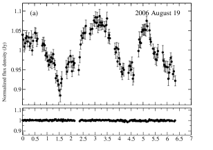
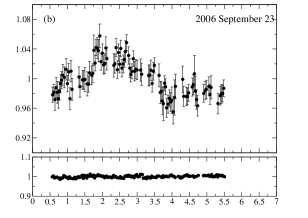
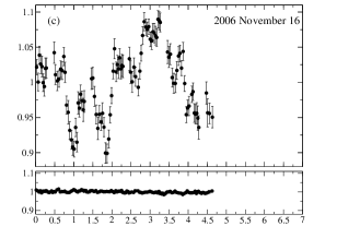
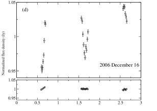
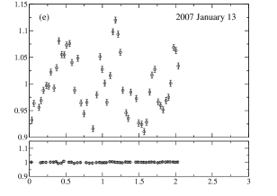
Figure 1: 4.85 GHz light curves of J1128+5925 (upper plots) and those of the secondary calibrator B0836+710 (lower plots) from 2006 August (panel (a) ) until 2007 January (panel (e) ). On the abscissa the observing time (in days) is displayed, the starting dates are given in the upper right corner of each plot. On the ordinate are the normalized flux densities in Jansky. Panels (a), (b) and (c) show Urumqi observations, panels (d) and (e) show Effelsberg observations.

In Fig. 1 the light curves of five new, previously unpublished IDV observations of J1128+592 are shown. As in all the previous measurements, J1128+592 showed pronounced variability with peak-to-trough amplitudes of up to 20-25 %.

The observed variability time scales of J1128+592 are significantly different at different dates (see Col. 5 of Table 1). In Gabányi et al. (2007), we proposed that the changes in the characteristic variability time scale may be due to annual modulation. The best fit to the data was achieved using the anisotropic annual modulation model of Bignall et al. (2006), which is represented by the solid curve in Fig. 2.

In the anisotropic model, the scintillation time scale also depends on the ellipticity of the scintillation pattern and on the direction in which the relative velocity vector (between the Earth and the screen) “cuts through” the elliptical scintillation pattern. Thus, the fitted parameters obtained from the anisotropic scintillation model are the velocity components of the scattering screen, the scattering length-scale (which depends on the screen distance and the scattering angle), the angular ratio of the anisotropy and its position angle.

However, not all of the new observations (data points at day 234, day 267, day 309 and day 13) fit equally well to this model. It is clear that the time scales derived from the observation in September 2005 and in September 2006 do not agree well with each other, questioning the interpretation via annual modulation. The larger error bar on the time scale obtained in September 2006 is due to the fact that only one well-defined variability peak occurred during this observation. Moreover the relatively slow time scale as measured in November 2006 (day 309) does not agree well with the model. On the other hand, the acceleration of the variability time scale, which is expected after autumn (day $\geq 240$) is basically seen again, also with the new data. Despite some difficulties in the determination of the time scale in December 2006 (due to irregular sampling), the variability in this months is faster than in autumn. Also the measurements of January 2007 (day 13) are consistent with such fast variability, although this recent data point shows a bit slower variations than in February 2006 (see Fig. 1).

Inspecting the structure function and autocorrelation
function of the 2006 November data reveals a possible faster time scale of $\sim 0.5$ day. This time scale would fit to the model. Unfortunately the sampling and the amount of measurements obtained in the later epoch, in 2006 December are not adequate to check the existence of two time scales. At the previous epoch (2006 September), there is no sign of variation on an additional time scale either. More observations are necessary to confirm or reject the appearance of a secondary time scale.

Apart from the time scale, the modulation index shows significant variations as well. Notably, in 2006 September the modulation index is half of the one measured in the previous epoch (2006 August) and the following epoch (2006 November). In the latter case $m=4.7$ %, whilst in September $m=2.3$ %. The annual modulation model cannot explain changes in the strength of variability. These different variability indices might therefore suggest changes in the scattering plasma or intrinsic changes in the source. If the scattering angle or the intrinsic source size has increased in this epoch, we would expect a prolongation of the time scale as well. So this might explain the discrepancy with the annual modulation model.

Finally, we note that the mean flux density at 4.85 GHz changed significantly during the $\sim 2$ years of monitoring of J1128+592. The flux density increased by $\sim 27$ % until 2006 February, then monotonously decreased until our last observation to approximately the same flux-density level. This long term flux density change suggests a source-intrinsic origin (e.g. an ejection of a new jet component), which could influence the variability behavior of the source on IDV time scales as well. Already proposed Effelsberg monitoring observations will help us to further investigate these questions. Additionally, proposed Very Long Baseline Array observations can reveal any intrinsic changes in the radio structure of J1128+592.

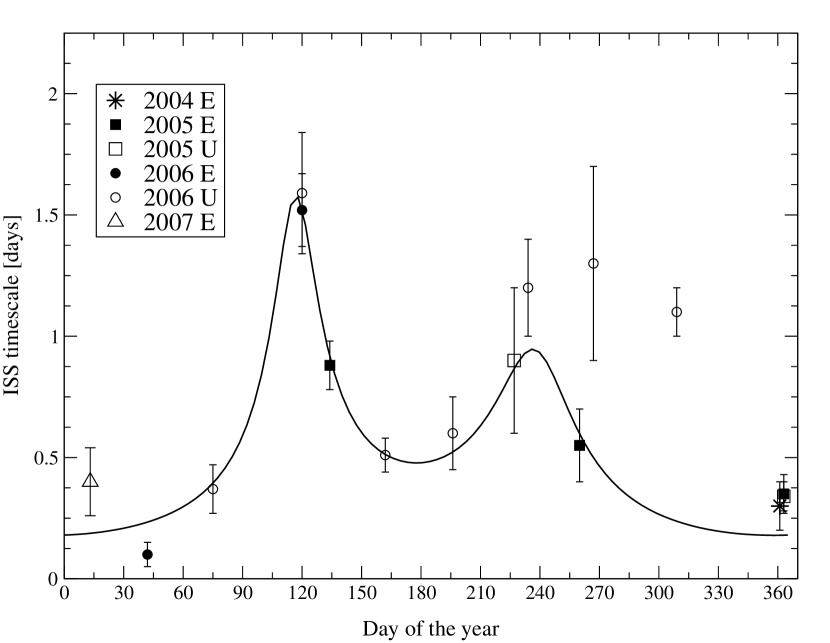
Figure 2: The characteristic variability time scales of J1128+592 plotted versus day of the year. The data are from 4.85 GHz observations performed with the Effelsberg telescope (filled symbols) and with the Urumqi telescope (open symbols). Different symbols represent observations performed in different years: star stands for 2004, squares for 2005, circles for 2006 and triangle for 2007. The solid curve represents the best fit annual modulation model as given in Gabányi et al. (2007), which uses only the first ten observing epochs for the fit.