Optimal Delay-Throughput Trade-offs in Mobile Ad-Hoc Networks:
Hybrid Random Walk and One-Dimensional Mobility Models

Abstract

Optimal delay-throughput trade-offs for two-dimensional i.i.d mobility models have been established in [23], where we showed that the optimal trade-offs can be achieved using rate-less codes when the required delay guarantees are sufficient large. In this paper, we extend the results to other mobility models including two-dimensional hybrid random walk model, one-dimensional i.i.d. mobility model and one-dimensional hybrid random walk model. We consider both fast mobiles and slow mobiles, and establish the optimal delay-throughput trade-offs under some conditions. Joint coding-scheduling algorithms are also proposed to achieve the optimal trade-offs.

I Notations

The following notations are used throughout this paper, given non-negative functions $f(n)$ and $g(n)$:

1. $f(n)=O(g(n))$ means there exist positive constants $c$ and $m$ such that $f(n)\leq cg(n)$ for all $n\geq m$.

2. $f(n)=\Omega(g(n))$ means there exist positive constants $c$ and $m$ such that $f(n)\geq cg(n)$ for all $n\geq m.$ Namely, $g(n)=O(f(n))$.

3. $f(n)=\Theta(g(n))$ means that both $f(n)=\Omega(g(n))$ and $f(n)=O(g(n))$ hold.

4. $f(n)=o(g(n))$ means that $\lim_{n\rightarrow\infty}f(n)/g(n)=0.$

5. $f(n)=\omega(g(n))$ means that $\lim_{n\rightarrow\infty}g(n)/f(n)=0.$ Namely, $g(n)=o(f(n)).$

II Introduction

Delay-throughput trade-offs in mobile ad-hoc networks have received much attention since the work of Grossglauser and Tse [9], where they showed that the throughput of ad-hoc networks can be significantly improved by exploring the node mobility. Recently the trade-off was investigated under different mobility models, which include the i.i.d. mobility [16, 21, 12, 23], one-dimensional mobility [3, 8], random walk [5, 6, 7, 19], hybrid random walk [19] and Brownian motion [13].

In [23], we demonstrated that the optimal trade-offs for two-dimensional i.i.d. mobility models can be achieved using rate-less codes when the required delay guarantees are sufficiently large. In this paper, we extend the results to the two-dimensional hybrid random walk, one-dimensional i.i.d. mobility and one-dimensional hybrid random walk models. The two-dimensional i.i.d. mobility studied in [23] only models the case where the network topology changes dramatically at each time slot. However Markovian mobility dynamics may be more realistic. Thus the two-dimensional hybrid random walk model was introduced by Sharma et al in [19], where the unit square is divided into $1/S^{2}$ small-squares, and mobiles move from the current small-square to one of its eight adjacent small-squares at the beginning of each time slot (The detailed description of the two-dimensional hybrid random walk model is presented in Section III). Since the distance each mobile can move is at most $2\sqrt{2}/S$ at each time slot, we can use different values of $S$ to model mobiles with different speeds, so this two-dimensional hybrid random walk model can be used for a wide range of scenarios. Note that the two-dimensional hybrid random walk model is the same as the two-dimensional i.i.d. mobility model when $S=1.$ One might wonder why the results in [23] are necessary given the results in this paper. The reason is that the Markovian mobility dynamics in this paper requires a different set of tools than those in [23] and as a result, the trade-off in this paper are applicable only when $S=o(1).$ Thus, the results in [23] cannot be recovered from the results of this paper. We wish to comment that one of the main differences between this paper and [23] is that, the i.i.d. mobility assumption in [23] allows us to use Chernoff bounds to obtain concentration results. However, the random walk and other mobility models in this paper require the use of martingale inequalities to establish the travel patterns of the mobiles.

In this paper, we will also study one-dimensional mobility models. These models are motivated by certain types of delay-tolerant networks [22], in which a satellite sub-network is used to connect local wireless networks outside of the Internet. Since the satellites move in fixed orbits, they can be modelled as one-dimensional mobilities on a two-dimensional plane. Motivated by such a delay-tolerant network, we consider one-dimensional mobility model where $n$ nodes move horizontally and the other $n$ node move vertically. Since the node mobility is restricted to one dimension, sources have more information about the positions of destinations compared with the two-dimensional mobility models. We will see that the throughput is improved in this case; for example, under the one-dimensional i.i.d. mobility model with fast mobiles, the trade-off will be shown to be $\Theta(\sqrt[3]{D^{2}/n}),$ which is better than $\Theta(\sqrt{D/n}),$ the trade-off under the two-dimensional i.i.d. mobility model with fast mobiles. We also propose joint coding-scheduling algorithms which achieve the optimal trade-offs.

Three mobility models are included in this paper, and each model will be investigated under both the fast-mobility and slow-mobility assumptions. The detailed analysis of the two-dimensional hybrid random walk model and one-dimensional i.i.d. mobility model will be presented. The results of the one-dimensional hybrid random walk model can be obtained using the techniques used in the other two models, so the analysis is omitted in this paper for brevity. Our main results include the followings:

1. Two-dimensional hybrid random walk model:

   1. Under the fast mobility assumption, it is shown that the maximum throughput per S-D pair is $O(\sqrt{D/n})$ when $S=o(1)$ and $D=\omega(|\log S|/S^{2}),$ and Joint Coding-Scheduling Algorithm I [23] can achieve the maximum throughput when $S=o(1)$ and $D$ is both $\omega(\max\{(\log^{2}n)|\log S|/S^{6},\sqrt[3]{n}\log n\})$ and $o(n/\log^{2}n).$

   2. Under the slow mobility assumption, it is shown that the maximum throughput per S-D pair is $O(\sqrt[3]{D/n})$ when $S=o(1)$ and $D=\omega(|\log S|/S^{2}),$ and Joint Coding-Scheduling Algorithm II can achieve the maximum throughput when $S=o(1)$ and $D$ is both $\omega((\log^{2}n)|\log S|/S^{6})$ and $o(n/\log^{2}n).$

2. One-dimensional i.i.d. mobility model:

   1. Under the fast mobility assumption, it is shown that the maximum throughput per S-D is $O\left(\sqrt[3]{D^{2}/n}\right)$ given delay constraint $D.$ Then Joint Coding-Scheduling Algorithm III is proposed to achieve the maximum throughput when $D$ is both $\omega(\sqrt[5]{n})$ and $o\left(\sqrt{n}/\sqrt[3/2]{\log n}\right).$

   2. Under the slow mobility assumption, it is shown that the maximum throughput per S-D pair is $O\left(\sqrt[4]{D^{2}/n}\right).$ Joint Coding-Scheduling Algorithm IV is proposed to achieve the maximum throughput when $D$ is $o\left(\sqrt{n}/\log^{2}n\right).$

3. One-dimensional hybrid random walk model:

   1. Under the fast mobility assumption, it is shown that the maximum throughput per S-D pair is $O(\sqrt[3]{D^{2}/n})$ when $S=o(1)$ and $D=\omega(1/S^{2}),$ and Joint Coding-Scheduling Algorithm III can achieve the maximum throughput when $S=o(1)$ and $D$ is both $\omega(\max\{(\log^{2}n)|\log S|/S^{4},\sqrt[5]{n}\log n\})$ and $o(\sqrt{n}/\sqrt[3/2]{\log n}).$

   2. Under the slow mobility assumption, it is shown that the maximum throughput per S-D pair is $O(\sqrt[4]{D^{2}/n})$ when $S=o(1)$ and $D=\omega(1/S^{2}),$ and Joint Coding-Scheduling Algorithm IV can achieve the maximum throughput when $S=o(1)$ and $D$ is both $\omega((\log^{2}n)|\log S|/S^{4})$ and $o(\sqrt{n}/\log^{2}n).$

Note that the optimal delay-throughput trade-off are established under some conditions on $D.$ When these conditions are not met, the trade-off is still unknown in general, though a trade-off of the two-dimensional hybrid random walk model with slow mobiles has been established under an assumption regarding packet replication in [19]. We also would like to mention that when the step size of the two-dimensional hybrid random walk is $1/\sqrt{n},$ our two-dimensional hybrid random walk model is identical to the random walk model studied in [6, 7], where the optimal delay-throughput trade-off has been obtained. Our results do not apply to this case since the set of allowed values for $D$ becomes empty in that case (see (1) (i) above).

The remainder of the paper is organized as follows: In Section III, we introduce the communication and mobility model. Then we analyze the two-dimensional hybrid random walk models in Section IV, and one-dimensional i.i.d. mobility models in Section V. The results of one-dimensional hybrid random walk model are presented in Section VI. Finally, the conclusions is given in Section VII.

III Model

In this section, we first present the models that we use for mobility and wireless interference. Then the definitions of delay and throughput are provided.

Mobile Ad-Hoc Network Model: Consider an ad-hoc network where wireless mobile nodes are positioned in a unit square. Assume that the time is slotted, we study following three mobility models in this paper.

1. Two-Dimensional Random Walk Model: Consider a unit square which is further divided into $1/S^{2}$ squares of equal size. Each of the smaller square will be called an RW-cell (random walk cell), and indexed by $(U^{x},U^{y})$ where $U^{x},U^{y}\in\{1,\ldots,1/S\}.$ The unit square is assumed to be a torus, i.e., the top and bottom edges are assumed to touch each other and similarly the left and right edges also are assumed to touch other. A node which is in one RW-cell at a time slot moves to one of its eight adjacent RW-cells or stays in the same RW-cell in the next time-slot with each move being equally likely as in Figure 1. Two RW-cells are said to be adjacent if they share a common point. The node position within the RW-cell is randomly uniformly selected. There are $n$ S-D pairs in the network. Each node is both a source and a destination. Without loss of generality, we assume that the destination of node $i$ is node $i+1,$ and the destination of node $n$ is node $1.$

   

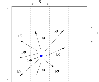
   Figure 1: Two-Dimensional Random Walk Model

2. One-Dimensional I.I.D. Mobility Model: Our one-dimensional i.i.d. mobility model is defined as follows:

   1. There are $2n$ nodes in the network. Among them, $n$ nodes, named H-nodes, move horizontally; and the other $n$ nodes, named V-nodes, move vertically.

   2. Using $(x_{i},y_{i})$ to denote the position of node $i.$ If node $i$ is an H-node, $y_{i}$ is fixed and $x_{i}$ is a value randomly uniformly chosen from $[0,1].$ We also assume that H-nodes are evenly distributed vertically, so $y_{i}$ takes values $1/n,2/n,\ldots,1.$ V-nodes have similar properties.

   3. Assume that source and destination are the same type of nodes. Also assume that node $i$ is an H-node if $i$ is odd, and a V-node if $i$ is even. Further, assume that the destination of node $i$ is node $i+2,$ the destination of node $2n-1$ is node $1,$ and the destination of node $2n$ is node $2.$

   4. The orbit distance of two H(V)-nodes is defined to be the vertical (horizontal) distance of the two nodes.

3. One-Dimensional Random Walk Model: Each orbit is divided into $1/S$ RW-intervals (random walk interval). At each time slot, a node moves into one of two adjacent RW-intervals or stays at the current RW-interval (see Figure 2). The node position in the RW-interval is randomly, uniformly selected.

   

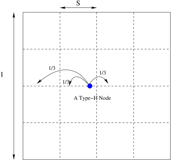
   Figure 2: One-Dimensional Random Walk Model

Communication Model: We assume the protocol model introduced in [10] in this paper. Let $\hbox{dist}(i,j)$ denote the Euclidean distance between node $i$ and node $j,$ and $r_{i}$ to denote the transmission radius of node $i.$ A transmission from node $i$ can be successfully received at node $j$ if and only if following two conditions hold:

1. $\hbox{dist}(i,j)\leq r_{i};$

2. $\hbox{dist}(k,j)\geq(1+\Delta)\hbox{dist}(i,j)$ for each node $k\not=i$ which transmits at the same time, where $\Delta$ is a protocol-specified guard-zone to prevent interference.

We further assume that at each time slot, at most $W$ bits can be transmitted in a successful transmission.

Time-Scale of Mobility: Two time-scales of mobility are considered in this paper.

1. Fast mobility: The mobility of nodes is at the same time-scale as the data transmission, so $W$ is a constant independent of $n$ and only one-hop transmissions are feasible in single time slot.

2. Slow mobility: The mobility of nodes is much slower than the wireless transmission, so $W\gg n.$ Under this assumption, the packet size can be scaled as $W/H(n)$ for $H(n)=O(n)$ to guarantee $H(n)$-hop transmissions are feasible in single time slot.

Delay and Throughput: We consider hard delay constraints in this paper. Given a delay constraint $D,$ a packet is said to be successfully delivered if the destination obtains the packet within $D$ time slots after it is sent out from the source.

Let $\Lambda_{i}[T]$ denote the number of bits successfully delivered to the destination of node $i$ in time interval $[0,T].$ A throughput of $\lambda$ per S-D pair is said to be feasible under the delay constraint $D$ and loss probability constraint $\epsilon>0$ if there exists $n_{0}$ such that for any $n\geq n_{0},$ there exists a coding/routing/scheduling algorithm with the property that each bit transmitted by a source is received at its destination with probability at least $1-\epsilon,$ and

$$\lim_{T\rightarrow\infty}\Pr\left(\displaystyle\frac{\Lambda_{i}[T]}{T}\geq\lambda,\hbox{ }\forall\hbox{ }i\right)=1.$$ (1)

IV Two-Dimensional Hybrid Random Walk Models

The optimal delay-throughput trade-offs of the two-dimensional i.i.d. mobility model with fast mobiles and slow mobiles have been established in [23]. In this section, we first first extend the results to two-dimensional hybrid random walk models. We will obtain the maximum throughput for $D=\omega\left(|\log S|/S^{2}\right),$ and then show that the maximum throughput can be achieved using the algorithms proposed in [23] under some additional constraints on $D.$

IV-A Upper Bound

The upper bound is established under the following assumptions:

Assumption 1: Packets destined for different nodes cannot be encoded together.

Assumption 2: A new coded packet is generated right before the packet is sent out. The node generating the coded packet does not store the packet in its buffer.

Assumption 3: Once a node receives a packet (coded or uncoded), the packet is not discarded by the node till its deadline expires.

Note that Assumption $1$ is the only significant restriction imposed on coding/routing/scheduling schemes. Next we introduce following notations which will be used in our proof.

• $\Lambda[T]:$ $\Lambda[T]=\sum_{i=1}^{n}\Lambda_{i}[T].$

• $b:$ Index of a bit stored in the network. Bit $b$ could be either a bit of a data packet or a bit of a coded packet.

• $d_{b}:$ The destination of bit $b.$

• $c_{b}:$ The node storing bit $b.$

• $t_{b}:$ The time slot at which bit $b$ is generated.

• $\tilde{L}_{b}:$ The minimum distance between node $d_{b}$ and node $c_{b}$ from time slot $t_{b}$ to time slot $t_{b}+D-1,$ i.e.,

  $$\tilde{L}_{b}=\min_{t_{b}\leq t\leq t_{b}+D-1}\hbox{dist}(d_{b},c_{b})(t).$$

Theorem 1

Consider the two-dimensional hybrid random walk model with step-size $S=o(1)$ and delay constraint $D=\omega(|\log S|/S^{2}),$ and suppose that Assumption 1-3 hold. We have following results:

1. For fast mobiles,

   $$\frac{48\sqrt{2}WT}{\Delta\sqrt{\pi}}\sqrt{n}(\sqrt{D}+1)\geq E[\Lambda[T]].$$ (2)

2. For slow mobiles,

   $$\frac{8\sqrt[3]{9}WT}{\sqrt[3/2]{\Delta\pi^{2}}}\sqrt[3/2]{n}(\sqrt[3]{D}+1)\geq E[\Lambda[T]].$$ (3)

Proof:

Let $N^{\rm rw}_{b}$ denote the number of time slots, from $t_{b}+1$ to $t_{b}+D,$ at which node $c_{b}$ and $d_{b}$ are in the same RW-cell or neighboring RW-cells. Then for any $L\in[0,S/\sqrt{\pi}),$ we have

$$\Pr\left(\tilde{L}_{b}\leq L\right)$$

$$= \sum_{K=1}^{D}\Pr\left(\tilde{L}_{b}\leq L|{N}^{\rm rw}_{b}=K\right)\Pr\left(N^{\rm rw}_{b}=K\right)$$

$$\leq \sum_{K=1}^{D}\left(1-\left(1-\frac{\pi L^{2}}{S^{2}}\right)^{K}\right)\Pr\left(N^{\rm rw}_{b}=K\right)$$

$$= 1-E\left[\left(1-\frac{\pi L^{2}}{S^{2}}\right)^{N^{\rm rw}_{b}}\right]$$

$$\leq 1-\left(1-\frac{\pi L^{2}}{S^{2}}\right)^{E\left[N^{\rm rw}_{b}\right]},$$

where the first inequality follows from the fact that the node position within a RW-cell is randomly uniformly selected, and the last inequality follows from the Jensen’s inequality.

Next we consider $E[N_{b}^{\rm tw}].$ Let $(U_{i}^{x}(t),U_{i}^{y}(t))$ denote the RW-cell in which node $i$ is at time slot $t,$ and $(V^{x}_{i}(t),V^{y}_{i}(t))$ denote the displacement of node $i$ at time slot $t,$ i.e.,

$$V^{x}_{i}(t)=\left\{\begin{array}[]{ll}1,&\hbox{w.p. }\frac{1}{3}\\ 0,&\hbox{w.p. }\frac{1}{3}\\ -1,&\hbox{w.p. }\frac{1}{3}\\ \end{array}\right.\hbox{ and }V^{y}_{i}(t)=\left\{\begin{array}[]{ll}1,&\hbox{w.p. }\frac{1}{3}\\ 0,&\hbox{w.p. }\frac{1}{3}\\ -1,&\hbox{w.p. }\frac{1}{3}\\ \end{array}\right..$$

It is easy to see that

$$U_{i}^{x}(t) = \left[\left(U_{i}^{x}(0)+\sum_{m=1}^{t-1}V^{x}_{i}(m)\right)\mod{\frac{1}{S}}\right]+1;$$

$$U_{i}^{y}(t) = \left[\left(U_{i}^{y}(0)+\sum_{m=1}^{t-1}V^{y}_{i}(m)\right)\mod{\frac{1}{S}}\right]+1.$$

Further, let $(U_{i-j}^{x}(t),U_{i-j}^{y}(t))$ denote the relative position of node $i$ from node $j,$ i.e.,

$$U_{i-j}^{x}(t) = \left(U_{i-j}^{x}(0)+\sum_{m=1}^{t-1}\tilde{V}^{x}_{i-j}(m)\right)\mod{\frac{1}{S}};$$

$$U_{i-j}^{y}(t) = \left(U_{i-j}^{y}(0)+\sum_{m=1}^{t-1}\tilde{V}^{y}_{i-j}(m)\right)\mod{\frac{1}{S}},$$

where

$$\tilde{V}^{x}_{i-j}(t)={V}^{x}_{i}(t)-{V}^{x}_{j}(t)=\left\{\begin{array}[]{ll}2,&\hbox{w.p. }\frac{1}{9}\\ 1,&\hbox{w.p. }\frac{2}{9}\\ 0,&\hbox{w.p. }\frac{1}{3}\\ -1,&\hbox{w.p. }\frac{2}{9}\\ -2,&\hbox{w.p. }\frac{1}{9}\\ \end{array}\right.,$$

and

$$\tilde{V}^{y}_{i-j}(t)={V}^{y}_{i}(t)-{V}^{y}_{j}(t)=\left\{\begin{array}[]{ll}2,&\hbox{w.p. }\frac{1}{9}\\ 1,&\hbox{w.p. }\frac{2}{9}\\ 0,&\hbox{w.p. }\frac{1}{3}\\ -1,&\hbox{w.p. }\frac{2}{9}\\ -2,&\hbox{w.p. }\frac{1}{9}\\ \end{array}\right..$$

So $(U_{i-j}^{x}(t),U_{i-j}^{y}(t))$ is the consequence of random walk $(\tilde{V}^{x}_{i-j}(m),\tilde{V}^{y}_{i-j}(m))$ with initial position

$$(U_{i-j}^{x}(0),U_{i-j}^{y}(0))=(U_{i}^{x}(0)-U_{j}^{x}(0),U_{i}^{y}(0)-U_{j}^{y}(0)).$$

Note that node $c_{b}$ and node $d_{b}$ are in the same RW-cell if $(U_{c_{b}-d_{b}}^{x}(t),U_{c_{b}-d_{b}}^{y}(t))=(0,0),$ and in neighboring RW-cells if $(U_{c_{b}-d_{b}}^{x}(t),U_{c_{b}-d_{b}}^{y}(t))\in\{(0,1),(1,0),(1,1),(0,1/S-1),(1/S-1,0),(1/S-1,1/S-1)\}.$ Similar to the argument in Lemma 12 provided in Appendix B, we can conclude that for $D=\omega(|\log S|/S^{2}),$

$$E\left[N^{\rm rw}_{b}\right]\leq\frac{99}{10}S^{2}D,$$

which implies that

$$\Pr\left(\tilde{L}_{b}\leq L\right) \leq 1-\left(1-\frac{\pi L^{2}}{S^{2}}\right)^{\frac{99}{10}S^{2}D}$$ (7)

$$\leq 36L^{2}D.$$

Based on inequality (7), the proof of inequality (2) is similar to the proof of Theorem 3 of [23], and the proof of (3) is similar to the proof of Theorem 6 of [23]. ∎

IV-B Joint Coding-Scheduling Algorithms

From Theorem 1, we can see that the optimal delay-throughput trade-offs of the two-dimensional hybrid random walk models are similar to the ones of the two-dimensional i.i.d. mobility models [23]. It motivates us to consider the algorithms proposed in [23]. As in [23], we define and categorize packets into four different types.

• Data packets: There are the uncoded data packets that have to be transmitted by the sources and received by the destinations.

• Coded packets: Packets generated by Raptor codes. We let $(i,k)$ denote the $k^{\rm th}$ coded packet of node $i.$

• Duplicate packets: Each coded packet could be broadcast to other nodes to generate multiple copies, called duplicate packets. We let $(i,k,j)$ denote a copy of $(i,k)$ carried by node $j,$ and $(i,k,J)$ to denote the set of all copies of coded packet $(i,k).$

• Deliverable packets: Duplicate packets that happen to be within distance $L$ from their destinations.

We will show that the optimal trade-offs can be achieved using Joint Coding-Scheduling Algorithm I and II presented in [23] with the following modifications:

1. For the fast mobility model, we use Joint Coding-Scheduling Algorithm I with the following modification: $2D/(25M)$ data packets are coded into $D/M$ coded packets;

2. For the slow mobility model, we use Joint Coding-Scheduling Algorithm II with the following modifications: $D/7$ data packets are coded to $D$ coded packets.

For the detail of the algorithms, please refer to [23].

Theorem 2

Consider the two-dimensional hybrid random walk models.

1. Fast mobility model: Suppose that $S$ is $o(1),$ $D$ is both $\omega(\max\{\log^{2}n|\log S|/(S^{6}),\sqrt[3]{n}\log n\})$ and $o(n/(\log^{2}n)),$ and the delay constraint is $6D.$ Then under the fast mobility model, given any $\epsilon$ there exists $n_{0}$ such that for any $n\geq n_{0},$ every data packet sent out can be recovered at the destination with probability at least $1-\epsilon,$ and

   $$\lim_{T\rightarrow\infty}\Pr\left(\frac{\Lambda_{i}[T]}{T}\geq\left(\frac{W}{2520}\right)\left(\sqrt{\frac{D}{n}}\right)\hbox{ }\forall i\right)=1.$$ (8)

   by using the modified Joint Coding-Scheduling Algorithm I.

2. Slow mobility model: Suppose that $S$ is $o(1)$ and $D$ is both $\omega(\log^{2}n|\log S|/(S^{6}))$ and $o(n/(\log^{3}n)),$ and the delay constraints is $16D.$ Then under the slow mobility model, given any $\epsilon$ there exists $\tilde{n}_{0}$ such that for any $n\geq\tilde{n}_{0},$ every data packet sent out can be recovered at the destination with probability at least $1-\epsilon,$ and

   $$\lim_{T\rightarrow\infty}\Pr\left(\frac{\Lambda_{i}[T]}{T}\geq\left(\frac{W}{224\sqrt{2}c_{s}C}\right)\left(\sqrt[3]{\frac{D}{n}}\right)\hbox{ }\forall i\right)=1.$$ (9)

   by using the modified Joint Coding-Scheduling Algorithm II.

Proof:

Let $\tilde{A}$ denote the area of a cell, and $\tilde{M}[t]$ to denote the number of nodes in the cell at time slot $t.$ A cell is said to be a good cell at time $t$ if

$$\frac{9}{10}\tilde{A}n+1\leq\tilde{M}[t]\leq\frac{11}{10}{\tilde{A}n}.$$

Proof of (1): We consider one super time slot which consists of $6D$ time slots, and calculate the probability that the $2D/(25M)$ data packets from node $i$ are fully recovered at the destination, where $M=\sqrt{n/D}$ is the mean number of nodes in each cell. The proof will show the following events happen with high probability.

Node distribution: All cells are good during the entire super-time-slot with high probability. Letting $\cal G$ denote this event, we will show

$$\Pr\left({\cal G}\right)\geq 1-\frac{1}{n^{2}}.$$ (10)

Broadcasting: At least $16D/(25M)$ coded packets from a source are successfully duplicated after the broadcasting step with high probability, where a coded packet is said to be successfully duplicated if the packet is in at least $4M/5$ distinct relay nodes. Letting $A_{i}$ denote the number of coded packets which are successfully duplicated in a super time slot, we will first show that

$$\Pr\left(\left.A_{i}\geq\frac{16D}{25M}\right|{\cal G}\right)\geq 1-\frac{55D}{n}-e^{-\frac{D}{600M}}.$$ (11)

Receiving: At least $3D/(25M)$ distinct coded packets from a source are delivered to its destination after the receiving step with high probability. Letting $B_{i}$ denote the number of distinct coded packets delivered to destination $i+1$ in a super time slot, we will show

$$\Pr\left(\left.B_{i}\geq\frac{3}{25}\frac{D}{M}\right|A_{i}\geq\frac{16}{25}\frac{D}{M}\right)\geq 1-2e^{-\frac{\log D}{8500}}-e^{-\frac{D}{500M\log D}}.$$ (12)

From inequalities (10), (11) and (12), we can conclude that under the Joint Coding-Scheduling Algorithm I, at each super time slot, the $2D/(25M)$ data packets can be successfully recovered with probability at least

$$1-\frac{1}{n^{2}}-\frac{55D}{n}-e^{-\frac{D}{600M}}-2e^{-\frac{\log D}{8500}}-e^{-\frac{D}{500M\log D}}.$$

The rest of the proof is the same as the proof of Theorem 4 in [23].

Analysis of node distribution: Since $D=o\left(n/\log^{2}n\right)$ implies $M=\omega(\log n).$ Inequality (10) can be obtained from the Chernoff bound and union bound.

Analysis of broadcasting step: Consider the broadcasting step. Note that when ${\cal G}$ occurs, node $i$ is selected to broadcast with probability at least $10/(11M)$ at each time slot. Let ${\cal B}_{i}[t]$ denote the event that node $i$ is selected to broadcast in time slot $t.$ From the Chernoff bound, we have

$$\Pr\left(\left.\sum_{t=1}^{D}1_{{\cal B}_{i}[t]}\geq\frac{9}{11}\frac{D}{M}\right|{\cal G}\right)\geq 1-e^{-\frac{D}{600M}}.$$ (13)

So node $i$ broadcasts $9D/(11M)$ coded packets with a high probability. Each coded packet is broadcast to $9M/10$ relay nodes.

According to Step (2)(ii) of Joint Coding-Scheduling Algorithm I [23], each relay node keeps at most one packet for each source. Consider duplicate packet $(i,k,j).$ It could be dropped if node $j$ is in the same cell as node $i$ and node $i$ is selected to broadcast. Thus, the probability that $(i,k,j)$ is dropped is at most

$$\frac{11}{10}\frac{DM}{n}\times\frac{10}{9}\frac{1}{M}=\frac{11}{9}\frac{D}{n}$$ (14)

due to the following two facts:

1. Let ${\cal H}_{ji}[D]$ denote the event that node $j$ is in the same cell as node $i$ in at least one of $D$ consecutive time slots. Similar to (7), it can be shown that

   $$\Pr\left({{\cal H}_{ji}[D]}\right)\leq\frac{11}{10}\frac{DM}{n}$$ (15)

   under the delay constraint given in the theorem.

2. When ${\cal G}$ occurs, node $i$ is selected to broadcast with probability at most $10/(9M)$ at each time slot.

Now suppose source $i$ broadcasts $\tilde{D}_{i}$ coded packets, so $9M\tilde{D}_{i}/10$ duplicate copies are generated. Let $\tilde{N}^{d}_{i}$ denote the number of duplicate packets of node $i$ dropped in the broadcasting step. From the Markov inequality and inequality (14), we have

$$\Pr\left(\tilde{N}_{i}^{d}\geq\frac{M\tilde{D}_{i}}{50}\left|{\cal G},\sum_{t=1}^{D}1_{{\cal B}_{i}[t]}=\tilde{D}_{i}\right.\right)$$

$$\leq \frac{E\left[\tilde{N}_{i}^{d}\geq\frac{M\tilde{D}_{i}}{50}\left|{\cal G},\sum_{t=1}^{D}1_{{\cal B}_{i}[t]}=\tilde{D}_{i}\right.\right]}{\frac{M\tilde{D}_{i}}{50}}$$

$$\leq \frac{\frac{9M\tilde{D}_{i}}{10}\times\frac{11D}{9n}}{\frac{M\tilde{D}_{i}}{50}}$$

$$= \frac{55D}{n},$$

which implies

$$\Pr\left(A_{i}\geq\frac{4}{5}\tilde{D}_{i}\left|{\cal G},\sum_{t=1}^{D}1_{{\cal B}_{i}[t]}=\tilde{D}_{i}\right.\right)\geq 1-\frac{55D}{n}$$ (16)

since otherwise, more than $M\tilde{D}_{i}/50$ duplicate packets would be dropped. Inequality (11) follows from inequalities (16) and (13).

Analysis of receiving step: We group every $3D/\log D$ time slots into big time slots, named as b-time-slot and indexed by $t_{b},$ and then divided every b-time-slot into three equal parts, indexed by $t_{b,1},$ $t_{b,2}$ and $t_{b,3}$ as in Figure 3.

Figure 3: The Division of A Super Time Slot

We first calculate the probability that coded packet $(i,k)$ is delivered in $t_{b,2}.$ Let ${\cal H}_{(i,k)}[t_{b,2}]$ denote the event that at least one copy of packet $(i,k)$ becomes deliverable in $t_{b,2}.$ If $(i,k)$ is in at least $4M/5$ relay nodes, we can obtain

$$\Pr\left({{\cal H}_{(i,k)}\left[t_{b,2}\right]}\right) \geq 1-\left(\left(1-\frac{M}{nS^{2}}\right)^{\frac{4DS^{2}}{5\log D}}+\frac{1}{n}\right)^{\frac{4M}{5}}$$ (17)

$$\geq \frac{3}{5}\frac{1}{\log D}$$

due to the following facts:

1. Given $D/\log D=\omega(\log n|\log S|/S^{6}),$ from Lemma 12 provided in Appendix B, we know that with probability at least $1-1/n,$ two nodes are in the same RW-cell for at least $4DS^{2}/(5\log D)$ time slots.

2. Given two nodes are in the same RW-cell, the probability that they are in the same cell is $M/(nS^{2}).$

Next note that the duration of $t_{b,1}$ and $t_{b,3}$ are of a larger order than the mixing time of the random walk (the mixing time is defined in Appendix B). From the definition of the mixing time, we have that at any time slot belonging to $t_{b,2},$ the nodes are almost uniformly distributed in the unit square. Let ${\cal D}_{(i,k)}[t_{b,2}]$ denote the event that coded packet $(i,k)$ is delivered to its destination in $t_{b,2}.$ Following the argument used to prove inequality (13) of Theorem 4 in [23], we have

$$\Pr\left({{\cal D}_{(i,k)}[t_{b,2}]}\right)\geq\frac{3}{20\log D}.$$ (18)

Now let $\mathbf{x}_{t}$ denote the positions of the nodes at time slot $t,$ and

$$\tilde{\mathbf{X}}=\{{\mathbf{x}}_{t}\}_{t=\frac{3(k-1)D}{\log D}+1}$$

for $k=1,\ldots,5\log D/3.$ Also let ${\cal D}_{(i,k)}$ denote the event that $(i,k)$ is delivered in the receiving step. It is easy to see that ${\cal D}_{(i,k)}$ occurs if ${\cal D}_{(i,k)}[t_{b,2}]$ occurs for some $t_{b,2}\in\{1,\ldots,5\log D/3\}.$ Note that $\{{\cal D}_{(i,k)}[t_{b,2}]\}_{t_{b,2}}$ are mutually independent given $\tilde{\mathbf{X}},$ so from inequality (18), we have

$$\Pr\left(\left.{{\cal D}_{(i,k)}}\right|\tilde{\mathbf{X}}\right)\geq 1-\left(1-\frac{3}{20}\frac{1}{\log D}\right)^{5\log D/3}\geq\frac{1}{5}.$$

Further since $B_{i}\geq\sum_{k=1}^{A_{i}}1_{{\cal D}_{(i,k)}},$ we can conclude that

$$E\left[B_{i}\left|\tilde{\mathbf{X}},A_{i}\geq\frac{16}{25}\frac{D}{M}\right.\right]\geq\frac{16}{125}\frac{D}{M}.$$ (19)

We next bound the number of distinct coded packets deliverable in $t_{b}.$ Similar to inequality (17), we have

$$\Pr\left({{\cal H}_{(i,k)}\left[t_{b}\right]}\right)\leq\frac{3}{\log D}.$$

Note that no two duplicate packets from node $i$ are in one relay node, so $\{{\cal H}_{(i,k)}[t_{b}]\}_{k}$ are mutually independent. From the Chernoff bound, we have

$$\Pr\left(\sum_{k=1}^{D/M}1_{{\cal H}_{(i,k)}\left[t_{b}\right]}\leq\frac{16}{5}\frac{D}{M\log D}\right)\geq 1-e^{-\frac{D}{400M\log D}}.$$

Let $\tilde{{\cal F}}_{i}$ denote the event that node $i$ obtains no more than $16D/(5M\log D)$ coded packets at each b-time-slot in the receiving step. From the union bound, we have that for sufficiently large $n,$

$$\Pr\left({\tilde{{\cal F}}_{i}}\right)\geq 1-\left(\frac{5}{3}\log D\right)\left(e^{-\frac{D}{400M\log D}}\right)\geq 1-e^{-\frac{D}{500M\log D}}.$$ (20)

Now let $B_{i}(\tilde{\mathbf{X}},A_{i},{\cal F}_{i})$ denote the number of distinct coded packets delivered to the destination of node $i$ given $(\tilde{\mathbf{X}},A_{i},{\cal F}_{i}),$ and $\mathbf{X}_{t_{b}}$ denote an $n\times(3D/\log D)$ matrix where the $(i,t)$ entry is the position of node $i$ at the $t^{\rm th}$ time slot of b-time-slot $t_{b}.$ It is easy to see that the value of $B_{i}(\tilde{\mathbf{X}},A_{i},{\cal F}_{i})$ is determined by $\{\mathbf{X}_{t_{b}}\},$ i.e., there exists a function $f_{(\tilde{\mathbf{X}},A_{i},{\cal F}_{i})}$ such that

$$B_{i}(\tilde{\mathbf{X}},A_{i},{\cal F}_{i})=f_{(\tilde{\mathbf{X}},A_{i},{\cal F}_{i})}\left(\mathbf{X}_{1},\ldots,\mathbf{X}_{5\log D/3}\right).$$

From the definition of ${\cal F}_{i},$ function $f_{(\tilde{\mathbf{X}},A_{i},{\cal F}_{i})}$ satisfies the following condition,

$$\left|f_{(\tilde{\mathbf{X}},A_{i},{\cal F}_{i})}\left(\mathbf{X}_{1},\ldots,\mathbf{X}_{t_{b}-1},\mathbf{X}_{t_{b}},\mathbf{X}_{t_{b}+1},\ldots,\mathbf{X}_{5\log D/3}\right)-\right.$$

$$\left.f_{(\tilde{\mathbf{X}},A_{i},{\cal F}_{i})}\left(\mathbf{X}_{1},\ldots,\mathbf{X}_{t_{b}-1},\mathbf{Y}_{t_{b}},\mathbf{X}_{t_{b}+1},\ldots,\mathbf{X}_{5\log D/3}\right)\right|\leq \frac{16}{5}\frac{D}{M\log D}.$$ (21)

It is easy to see that $\{\mathbf{X}_{t_{b}}\}$ are mutually independent given $(\tilde{\mathbf{X}},A_{i},\tilde{{\cal F}}_{i}).$ Then invoking Azuma-Hoeffding inequality provided in Appendix A, we can conclude that

$$\Pr\left(B_{i}{(\tilde{\mathbf{X}},A_{i},{\cal F}_{i})}\geq E\left[B_{i}\left|\tilde{\mathbf{X}},A_{i},\tilde{{\cal F}}_{i}\right.\right]-\frac{1}{125}\frac{D}{M}\right)$$

$$\geq 1-2e^{-\frac{\log D}{8500}}$$ (22)

holds for any $\tilde{\mathbf{X}}$ and $A_{i}.$ Inequality (12) follows from inequalities (19), (20) and (22).

Proof of (2): We consider one super time slot which consists of $16D$ time slots, and calculate the probability that the $D/7$ data packets from node $i$ are fully recovered at the destination. Let $M_{1}=\sqrt[3]{n/D},$ which is the mean number of nodes in each cell at the broadcasting step. Following the analysis above, we can prove that the following events happen with high probability.

Node distribution: All cells are good during the entire super-time-slot with high probability, i.e.,

$$\Pr\left({\cal G}\right)\geq 1-\frac{1}{n^{2}}.$$

Broadcasting: At least $4D/5$ coded packets from a source are successfully duplicated after the broadcasting step with high probability. Specifically, we have

$$\Pr\left(\left.A_{i}\geq\frac{4}{5}D\right|{\cal G}\right)\geq 1-\frac{50}{M_{1}^{2}},$$ (23)

where a coded packet is said to be successfully duplicated if it is in $4M_{1}/5$ distinct relay nodes.

Receiving: At least $D/6$ distinct coded packets from a source are delivered to its destination after the receiving step with high probability. Specifically, we have

$$\Pr\left(\left.B_{i}\geq\frac{D}{6}\right|A_{i}\geq\frac{4}{5}D\right)\geq 1-2e^{-\frac{\log D}{800}}.$$ (24)

From inequalities (10), (23) and (24), we can conclude that under the modified Joint Coding-Scheduling Algorithm II, at each super time slot, the $D/7$ source packets can be successfully recovered with probability at least

$$1-\frac{1}{n^{2}}-\frac{50}{M_{1}^{2}}-2e^{-\frac{\log D}{800}},$$

and theorem holds. ∎

V One-Dimensional I.I.D. Mobility Models

V-A Upper Bounds

Theorem 3

Consider the one-dimensional i.i.d. mobility model, and assume that Assumption 1-3 hold. We have following results:

1. For fast mobiles,

   $$8WT\sqrt[3]{\frac{2}{\pi\Delta^{2}}}\sqrt[3/2]{n}(\sqrt[3/2]{D}+1)\geq E[\Lambda[T]];$$

2. For slow mobiles,

   $$4WT\sqrt[4]{\frac{4}{\pi\Delta^{2}}}\sqrt[3/4]{n}(\sqrt{D}+1)\geq E[\Lambda[T]].$$

Proof:

Recall that $\tilde{L}_{b}$ is the minimum distance between node $d_{b}$ and node $c_{b}$ from time slot $t_{b}$ to $t_{b}+D-1.$ If the orbits of node $c_{b}$ and $d_{b}$ are vertical to each other, then $\tilde{L}_{b}\leq L$ holds only if at some time slot $t,$ node $c_{b}$ and $d_{b}$ are in the square with side length $2L$ as in Figure 4. In this case, we have

$$\Pr\left(\tilde{L}_{b}\leq L\right)\leq 1-(1-4L^{2})^{D}.$$

If the orbits of node $c_{b}$ and $d_{b}$ are parallel to each other, then it is easy to verify that

$$\Pr\left(\tilde{L}_{b}\leq L\right)\leq 1-(1-2L)^{D}.$$

Thus for $L\leq 1/2,$ we can conclude that

$$\Pr\left(\tilde{L}_{b}\leq L\right)\leq 1-(1-2L)^{D}\leq 2LD.$$

The rest of the proof is similar to Theorem 3 and Theorem 6 in [23].

Figure 4: The Two Orbits are Vertical to Each Other

∎

V-B Joint Coding-Scheduling Algorithm for Fast Mobility

Choose

$$M=\sqrt[3]{\frac{n}{D^{2}}}.$$

We divide the unit square into $\sqrt{n/M}$ horizontal rectangles, named as H-rectangles; and $\sqrt{n/M}$ vertical rectangles, named as V-rectangles as in Figure 5. A packet is said to be destined to a rectangle if the orbit of its destination is contained in the rectangle.

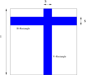
Figure 5: The Unit Square is Divided into H(V)-Rectangles

The algorithms for the one-dimensional i.i.d. mobility model has four steps. The first step is the Raptor encoding. The second step is the broadcasting step. In this step, the H(V)-nodes broadcast coded packets to V(H)-nodes. The third step is the transporting step, where the V(H)-nodes transport the H(V)-packets to the H(V)-rectangles containing the orbits of corresponding destinations, and then broadcast packets to the H(V)-nodes whose orbits are contained in the rectangles. After the third step, all duplicate packets are carried by the nodes that move parallel with the destinations and their orbit distance is less than $\sqrt{M/n}.$ The fourth step is the receiving step, where the packets are delivered to the destinations.

Since duplicate copies are generated in both the broadcasting step and the transporting step. To distinguish them, we name the duplicate packets generated at the broadcasting step as B-duplicate packets, and the duplicate packets generated at the transporting step as T-duplicate packets. Also we say a B-duplicate packet is transportable if it is in the rectangle containing the orbit of the destination of the packet.

Consider a cell with area $\tilde{A}$ and use $\tilde{M}^{H(V)}[t]$ to denote the number of H(V)-nodes in the cell. For the one-dimensional mobility model, a cell is said to be a good cell at time slot $t$ if

$$\frac{9}{10}\tilde{A}n+1\leq\tilde{M}^{H(V)}[t]\leq\frac{11}{10}\tilde{A}n.$$

Next we present the Joint Coding-Scheduling Algorithm III, which achieves the maximum throughput obtain in Theorem 4. Note that in the following algorithm, each time slot is further divide into $C$ mini-time slots, and each cell is guaranteed to be active in at least one of mini-time slot within each time slot.

Joint Coding-Scheduling Algorithm III: The unit square is divided into a regular lattice with $n/M$ cells, and the packet size is chosen to be $W/(2C).$ We group every $7D$ time slots into a super time slot. At each super time slot, the nodes transmit packets as follows.

1. Raptor Encoding: Each source takes $2D/(35M)$ data packets, and uses the Raptor codes to generate $D/M$ coded packets.

2. Broadcasting: This step consists of $D$ time slots. At each time slot, the nodes execute the following tasks:

   1. In each good cell, one H-node and one V-node are randomly selected. If the selected H(V)-node has never been in the current cell before and not already transmitted all of its $D/M$ coded packets, then it broadcasts a coded packet that was not previous transmitted to $9M/10$ V(H)-nodes in the cell during the mini-time slot allocated to that cell.

   2. All nodes check the duplicate packets they have. If more than one B-duplicate packets are destined to the same rectangle, randomly keep one and drop the others.

3. Transporting: This step consists of $D$ time slots. At each time slot, the nodes do the following:

   1. Suppose that node $j$ is a V-node ,and carries B-duplicate packet $(i,k,j).$ Node $j$ broadcasts $(i,k,j)$ to $9M/10$ H-nodes in the same cell if following conditions hold: (a) Node $j$ is in a good cell; (b) B-duplicate packet $(i,k,j)$ is the only transportable H-packet in the cell.

   2. Each node checks the T-duplicate packets it carries. If more than one T-duplicate packet has the same destination, randomly keep one and drop the others.

4. Receiving: This step consists of $5D$ time slots. At each time slot, if there are no more than two deliverable packets in the cell, the deliverable packets are delivered to the destinations with one-hop transmissions. At the end of this step, all undelivered packets are dropped. The destinations decode the received coded packets using Raptor decoding.

Theorem 4

Consider Joint Coding-Scheduling Algorithm III. Suppose $D$ is $\omega(\sqrt[5]{n})$ and $o\left(\sqrt{n}/\sqrt[3/2]{\log n}\right),$ and the delay constraint is $7D.$ Then given any $\epsilon>0,$ there exists $n_{0}$ such that for any $n\geq n_{0},$ every data packet sent out can be recovered at the destination with probability at least $1-\epsilon,$ and furthermore

$$\lim_{T\rightarrow\infty}\Pr\left(\frac{\Lambda_{i}[T]}{T}\geq\left(\frac{W}{980C}\right)\sqrt[3]{\frac{D^{2}}{n}}\hbox{ }\forall i\right)=1.$$

Proof:

Consider one super time slot and let $\cal G$ denote the event that all cells are good in the super time slot. The proof will show the following events happen with high probability.

Node distribution: All cells are good during the entire super-time-slot with high probability. Specifically, it is easy to verify that

$$\Pr\left({\cal G}\right)\geq 1-\frac{1}{n^{2}}.$$ (25)

Broadcasting: At least $2D/(3M)$ coded packets from a source are successfully duplicated after the broadcasting step with high probability, where a coded packet is said to be successfully duplicated if it has at least $4M/5$ B-duplicate packets. Specifically, we will show

$$\Pr\left(\left.A_{i}\geq\frac{2}{3}\frac{D}{M}\right|{\cal G}\right)\geq 1-\frac{40}{M}.$$ (26)

Transporting: At least $9D/(70M)$ coded packets from a source are successfully transported after the transporting step with high probability, where a coded packet is said to be successfully transported if it has at least $4M/5$ T-duplicate copies. Letting $C_{i}$ denote the number of successfully transported packets from node $i,$ we will show

$$\Pr\left(\left.C_{i}\geq\frac{9}{70}\frac{D}{M}\right|{\cal G},A_{i}\geq\frac{2}{3}\frac{D}{M}\right)\geq 1-3e^{-\frac{D}{1500M}}-\frac{100}{M^{2}}.$$ (27)

Receiving: At least $9D/(140M)$ distinct coded packets from a source are delivered to its destination after the receiving step. Specifically, we will show

$$\Pr\left(\left.B_{i}\geq\frac{9}{140}\frac{D}{M}\right|C_{i}\geq\frac{9}{70}\frac{D}{M}\right)\geq 1-2e^{-\frac{D}{8000M}}.$$ (28)

If the claims above hold, the probability that the $D/10M$ data packets are fully recovered in one super time slot is at least

$$1-\frac{1}{n^{2}}-\frac{40}{M}-3e^{-\frac{D}{1500M}}-\frac{100}{M^{2}}-2e^{-\frac{D}{8000M}}.$$

The theorem follows from a similar argument provided in Theorem 4 of [23].

Analysis of broadcasting step: Assume that ${\cal G}$ occurs, then at each time slot, node $i$ is selected with probability $10/(11M).$ Note that there are $\sqrt{n/M}$ cells on the orbit of node $i,$ and node $i$ is uniformly randomly positioned in one of the cells. Thus, the number of coded packets broadcast by node $i$ is equal to the number of non-empty bins of following balls-and-bins problem.

Balls-and-Bins Problem: Suppose we have $\sqrt{n/M}$ bins and one trash can. At each time slot, we drop a ball. Each bin receives the ball with probability $10/(11\sqrt{nM}),$ and the trash can receives the ball with probability $1-10/(11M).$ Repeat this $D$ times, i.e., $D$ balls are dropped.

From Lemma 9 provided in Appendix A, we have

$$\Pr\left(\left.\sum_{k=1}^{D}1_{{\cal B}_{i}[t]}\geq\frac{9D}{11M}\right|{\cal G}\right)\geq 1-e^{-\frac{3D}{1000M}}.$$

We say two nodes are competitive with each other if the orbits of their destinations are contained in the same rectangle, so each node has $\sqrt{Mn}-1$ competitive nodes. Suppose that node $i$ is an H-node and node $j$ is a V-node. Let $\tilde{N}^{c}_{i,j}(t)$ denote the number of node $i$’s competitive nodes in the V-rectangle containing the orbit of node $j$ at time slot $t.$ Since nodes are uniformly, randomly positioned on their orbits, from the Chernoff bound, we have

$$\Pr\left(\tilde{N}_{i,j}^{c}(t)\leq\frac{11}{10}M\right)\geq 1-e^{-\frac{M}{300}}.$$ (29)

Now consider B-duplicate packet $(i,k,j)$ and assume that node $z,$ a competitive of node $i,$ is in the V-rectangle containing the orbit of node $i.$ Then $(i,k,j)$ might be dropped when it is in the same cell as node $z,$ and node $z$ is selected to broadcast. The probability of this event is at most

$$\sqrt{\frac{M}{n}}\times\frac{10}{9M}.$$ (30)

From (29), (30) and the union bound, we can conclude that the probability that $(i,k,j)$ is dropped at time slot $t$ is at most

$$e^{-\frac{M}{300}}+\frac{11}{10}M\times\sqrt{\frac{M}{n}}\times\frac{10}{9M}=e^{-\frac{M}{300}}+\frac{11}{9}\sqrt{\frac{M}{n}},$$ (31)

which implies that the probability of $(i,k,j)$ dropped in the broadcasting step is at most

$$1-\left(1-e^{-\frac{M}{300}}-\frac{11}{9}\sqrt{\frac{M}{n}}\right)^{D}\leq De^{-\frac{M}{300}}+\frac{11}{9M}$$

Inequality (26) follows from above inequality and the Markov inequality.

Analysis of transporting step: Consider an H-node $i.$ Let $C_{(i,k)}$ denote the number of B-duplicate packets which are contained in the V-rectangle where $(i,k)$ broadcast, and are destined to the same H-rectangle as node $i.$ Note the following facts:

1. Each node has $\sqrt{Mn}-1$ competitive nodes.

2. Each H-node broadcasts at most $D/M$ coded packets. The probability that a coded packet broadcast in a specific V-rectangle is at most

   $$\frac{D}{M}\times\sqrt{\frac{M}{n}}=\frac{D}{\sqrt{nM}}.$$

3. Each broadcast generates $9M/10$ duplicate copies.

Thus, from the Chernoff bound, we have that

$$\Pr\left(C_{(i,k)}\leq DM\right)\geq 1-e^{-\frac{D}{300M}},$$

which implies that for sufficiently large $n,$

$$\Pr\left(C_{(i,k)}\leq DM\hbox{ }\forall\hbox{ }k\right)\geq 1-\frac{D}{M}e^{-\frac{D}{300M}}\geq 1-e^{-\frac{D}{400M}}.$$ (32)

Let ${\cal T}_{(i,k)}$ denote the event that a B-duplicate packet is broadcast at time slot $t$ in the transporting step. If $(i,k)$ is successfully duplicated, i.e., there are at least $4M/5$ B-duplicate copies of $(i,k),$ we have

$$\Pr\left({\cal T}_{(i,k)}(t)\right)\geq\frac{4M}{5}\sqrt{\frac{M}{n}}\left(1-\sqrt{\frac{M}{n}}\right)^{C_{(i,k)}+\frac{9M}{10}-1}.$$

Further, let ${\cal T}_{(i,k)}$ denote the event that at least one copy of $(i,k)$ is broadcast in the transporting step. Then for sufficiently large $n,$ we can obtain that

$$\Pr\left({{\cal T}_{(i,k)}}\left|C_{(i,k)}\leq DM\right.\right)$$

$$\geq 1-\left(1-\frac{4M}{5}\sqrt{\frac{M}{n}}\left(1-\sqrt{\frac{M}{n}}\right)^{DM+9M/10-1}\right)^{D}$$

$$\geq \frac{1}{4}.$$

Let $C^{b}_{i}$ denote the number of distinct coded packets of node $i$ broadcast in the transporting step, i.e.,

$$C^{b}_{i}=\sum_{k=1}^{D/M}1_{{\cal T}_{(i,k)}}.$$

Since different coded packets of node $i$ are broadcast in different V-rectangles, $\{{\cal T}_{(i,k)}\}$ are mutually independent. From the Chernoff bound, we have

$$\Pr\left(\left.C^{b}_{i}\geq\frac{D}{7M}\right|A_{i}\geq\frac{2D}{3M},C_{(i,k)}\leq MD\hbox{ }\forall k\right)\geq 1-2e^{-\frac{D}{900M}}.$$ (33)

In the transporting step, a T-duplicate copy will be dropped if the node carrying it obtains another packet destined to the same destination. Consider a T-duplicate packet $(i,k,l)$ carried by node $l.$ Note following facts:

1. Coded packets of node $i$ are broadcast in at most $D/M$ V-rectangles.

2. Each rectangle contains at most $9M/10$ B-duplicate copies from node $i.$

Thus, the probability of $(i,k,l)$ dropped at time slot $t$ is at most

$$\frac{D}{M}\sqrt{\frac{M}{n}}\left(1-\sqrt{\frac{M}{n}}\right)^{\frac{9M}{10}}$$

The node mobility is independent across time, so the probability of $(i,k,l)$ dropped in the transporting step is at most

$$1-\left(1-\frac{D}{M}\sqrt{\frac{M}{n}}\left(1-\sqrt{\frac{M}{n}}\right)^{\frac{9M}{10}}\right)^{D}\leq\frac{1}{M^{2}}.$$

Let $\bar{N}_{i}^{d}$ denote the number of duplicate packets dropped in the transporting step. Note that $9MC_{i}^{b}/10$ T-duplicate packets are generated, and each of them has probability $1/M^{2}$ to be dropped. Using the Markov inequality, we have

$$\Pr\left(\bar{N}_{i}^{d}\geq\frac{MC_{i}^{b}}{100}\right)\leq\frac{90}{M^{2}},$$

which implies

$$\Pr\left(C_{i}\geq\frac{9}{10}C_{i}^{b}\right)\geq 1-\frac{90}{M^{2}}$$ (34)

since otherwise, more than $MC_{i}^{b}/100$ duplicate copies are dropped. Inequality (27) follows form inequality (32)-(34).

Analysis of receiving step: The proof is similar to the proof of inequality (13) in [23]. ∎

V-C Joint Coding-Scheduling Algorithm for Slow Mobility

In this subsection, we propose an algorithm which achieves the delay-throughput trade-off obtained in Theorem 3. First choose

$$M_{1} = \sqrt[4]{\frac{n}{4D^{2}}}$$

$$M_{2} = M_{1}^{2}$$

and scale the packet size to be

$$\frac{W}{4c_{s}M_{1}}$$

where $c_{s}$ is a constant independent of $n$ as in [23]. Further, we divide the unit square into $\sqrt{n/M_{2}}$ horizontal rectangles, named as H-rectangles; and $\sqrt{n/M_{2}}$ vertical rectangles, named V-rectangles.

Joint Coding-Scheduling Algorithm IV: We group every $14D$ time slots into a super time slot. At each super time slot, the packets are coded and transmitted as follows:

1. Raptor Encoding: Each source takes $D/50$ data packets, and uses the Raptor codes to generate $D$ coded packets.

2. Broadcasting: The unit square is divided into a regular lattice with $n/M_{1}$ cells. This step consists of $D$ time slots. At each time slot, the nodes execute the following tasks:

   1. The nodes in good cells take their turns to broadcast. If node $i$ is a H(V)-node and has never been in the current cell before, it randomly selects $9M_{1}/10$ V(H)-nodes and broadcasts a coded packet to them.

   2. Each node checks the B-duplicate packets it carries. If there are multiple B-duplicate packets destined to the same rectangle, randomly pick one and drop the others.

3. Transporting: The unit square is divided into a regular lattice with $n/M_{1}$ cells. This step consists of $2D$ time slots. At each time slot, the nodes do the following:

   1. Suppose node $j$ carries duplicate packet $(i,k,j),$ which is an H-packet. If node $j$ is in a good cell and and $(i,k,j)$ is deliverable, node $j$ broadcasts the packet to $9M_{1}/10$ H-nodes in the cell.

   2. Each node checks the T-duplicate packets it carries. if there is more than one T-duplicate packet destined to the same destination, randomly pick one and drop the others.

4. Receiving: The unit square is divided into a regular lattice with $n/M_{2}$ cells. This step consists of $12D$ time slots. At each time slot, the nodes in good cells do the following at the mini-time slot allocated to their cells:

   1. The nodes which contain deliverable packets randomly pick one deliverable packet and send a request to the corresponding destination.

   2. For each destination, it accepts only one request.

   3. The nodes whose requests are accepted transmit the deliverable packets to their destinations using the highway algorithm proposed in [4].

   At the end of this step, all undelivered duplicate packets are dropped. Destinations use Raptor decoding to decode the received coded packets.

Theorem 5

Consider Joint Coding-Scheduling Algorithm IV. Suppose $D$ is both $\omega(1)$ and $o\left(\sqrt{n}/\log^{2}n\right),$ and the delay constraint is $14D.$ Then given any $\epsilon>0,$ there exists $n_{0}$ such that for any $n\geq n_{0},$ every data packet sent out can be recovered at the destination with probability $1-\epsilon,$ and furthermore

$$\lim_{T\rightarrow\infty}\Pr\left(\frac{\Lambda_{i}[T]}{T}\geq\left(\frac{W}{1400\sqrt{2}c_{s}C}\right)\sqrt[4]{\frac{D^{2}}{n}}\hbox{ }\forall i\right)=1.$$

Proof:

Following the analysis of Theorem 4, we can show the following events happen with high probability.

Node distribution: All cells are good during the entire super-time-slot with high probability, i.e.,

$$\Pr\left({\cal G}\right)\geq 1-\frac{1}{n^{2}}.$$ (35)

Broadcasting: At least $3D/10$ coded packets from a source are successfully duplicated after the broadcasting step with high probability, where a coded packet is said to be successfully duplicated if it has at least $M_{1}/3$ B-duplicate packets. Specifically, we have

$$\Pr\left(\left.A_{i}\geq\frac{3}{10}D\right|{\cal G}\right)\geq 1-\frac{1}{n^{2}}.$$ (36)

Transporting: At least $3D/40$ coded packets from a source are successfully transported after the transporting step with high probability, where a coded packet is said to be successfully transported if it has at least $4M_{1}/5$ T-duplicate copies. Specifically, we have

$$\Pr\left(\left.C_{i}\geq\frac{3}{40}D\right|{\cal G},A_{i}\geq\frac{3}{10}D\right)\geq 1-e^{-\frac{D}{3600}}-\frac{180}{\log n}.$$ (37)

Receiving: At least $D/40$ distinct coded packets from a source are delivered to its destination after the receiving step. Specifically, we have

$$\Pr\left(\left.B_{i}\geq\frac{D}{40}\right|{\cal G},C_{i}\geq\frac{3}{40}D\right)\geq 1-2e^{-\frac{D}{1000}}.$$ (38)

Thus, the probability that the $D/50$ data packets are fully recovered in one super time slot is at least

$$1-\frac{2}{n^{2}}-e^{-\frac{D}{3600}}-\frac{180}{\log n}-2e^{-\frac{D}{1000}},$$

and theorem holds. ∎

VI One-Dimensional Hybrid Random Walk Model, Fast Mobiles and Slow Mobiles

In this section, we present the optimal delay-throughput trade-offs of the one-dimensional hybrid random walk model. The results can be proved following the analysis of the one-dimensional i.i.d. mobility and the analysis of the two-dimensional hybrid random walk. The details are omitted here for brevity.

Theorem 6

Consider the one-dimensional hybrid random walk model and assume that Assumption 1-3 hold. Then for $S=o(1)$ and $D=\omega(1/S^{2}),$ We have following results:

1. For fast mobiles,

   $$24WT\sqrt[3]{\frac{1}{\pi\Delta^{2}}}\sqrt[3/2]{n}(\sqrt[3/2]{D}+1)\geq E[\Lambda[T]].$$ (39)

   When $S=o(1)$ and $D$ is both $\omega(\max\{(\log^{2}n)|\log S|/S^{4},\sqrt[5]{n}\log n\})$ and $o(\sqrt{n}/\sqrt[3/2]{\log n}),$ Joint Coding-Scheduling Algorithm III can be used to achieve a throughput same as (39) except for a constant factor.

2. For slow mobiles,

   $$12WT\sqrt[4]{\frac{1}{\pi\Delta^{2}}}\sqrt[3/4]{n}(\sqrt{D}+1)\geq E[\Lambda[T]].$$ (40)

   When $S=o(1)$ and $D$ is both $\omega((\log^{2}n)|\log S|/S^{4})$ and $o(\sqrt{n}/\log^{2}n),$ Joint Coding-Scheduling Algorithm IV can be used to achieve a throughput same as (40) except for a constant factor.

$\square$

VII Conclusion

In this paper, we investigated the optimal delay-throughput trade-off of a mobile ad-hoc network under the two-dimensional hybrid random walk, one-dimensional i.i.d. mobility model and one-dimensional hybrid random walk model. The optimal trade-offs have been established under some conditions on delay $D.$ When these conditions are not met, the optimal trade-offs are still unknown in general. We would like to comment that the key to establishing the optimal delay-throughput trade-off is to obtain $P_{i,j}(D,L),$ the probability that node $i$ hits node $j$ in one of $D$ consecutive time slots given a hitting distance $L.$ For example, under the two-dimensional hybrid random walk model, the upper bound was obtained under the condition $D=\omega(|\log S|/S^{2})$ since it was the condition under which we established an upper bound on $P_{i,j}(D,L)$ (inequality (7)). Further, the maximum throughput was shown to be achievable under a more restrict condition $D=\omega((\log^{2}n)|\log S|/S^{6})$ since it was the condition under which we established a lower bound on $P_{i,j}(D,L)$ (inequality (17)). Thus, if we can find techniques to compute $P_{i,j}(D,L)$ without using the restricts on $D,$ then the delay-throughput trade-offs can be characterized more generally. This is a topic for future research.

Acknowledgment: We thank Sichao Yang for useful discussions during the course of this work.

Appendix A: Probability Results

The following lemmas are some basic probability results.

Lemma 7

Let $X_{1},\ldots,X_{n}$ be independent $0-1$ random variables such that $\sum_{i}X_{i}=\mu.$ Then, the following Chernoff bounds hold

$$\hbox{Pr}\left(\sum_{i=1}^{n}X_{i}<(1-\delta)\mu\right) \leq e^{-\delta^{2}\mu/2};$$ (41)

$$\hbox{Pr}\left(\sum_{i=1}^{n}X_{i}>(1+\delta)\mu\right) \leq e^{-\delta^{2}\mu/3}.$$ (42)

Proof:

A detailed proof can be found in [15]. ∎

Lemma 8

Assume we have $m$ bins. At each time, choose $h$ bins and drop one ball in each of them. Repeat this $n$ times. Using $N_{1}$ to denote the number of bins containing at least one ball, the following inequality holds for sufficiently large $n.$

$$\hbox{Pr}\left(N_{1}\leq(1-\delta)m\tilde{p}_{1}\right) \leq 2e^{-\delta^{2}m\tilde{p}_{1}/3}.$$ (43)

where $\tilde{p}_{1}=1-e^{-\frac{nh}{m}}.$

Proof:

Please refer to [23] for a detailed proof. ∎

Lemma 9

Suppose $n$ balls are independently dropped into $m$ bins and one trash can. After a ball is dropped, the probability in the trash can is $1-p,$ and the probability in a specific bin is $p/m.$ Using $N_{2}$ to denote the number of bins containing at least $1$ ball, the following inequality holds for sufficiently large $n.$

$$\hbox{Pr}\left(N_{2}\leq(1-\delta)m\tilde{p}_{2}\right) \leq 2e^{-\delta^{2}m\tilde{p}_{2}/3};$$ (44)

where $\tilde{p}_{2}=1-e^{-\frac{np}{m}}.$

Proof:

Please refer to [23] for a detailed proof. ∎

Next we introduce the Azuma-Hoeffding inequality.

Lemma 10

Suppose that $X_{0},\ldots,X_{n}$ are independent random variables, and there exists a constant $c>0$ such that $f(\mathbf{X})=f(X_{1},\ldots,X_{n})$ satisfies the following condition for any $i$ and any set of values $x_{1},\ldots,x_{n}$ and $y_{i}:$

$$\left|f(x_{1},\ldots,x_{i-1},x_{i},x_{i+1},\ldots,x_{n})-\right.$$

$$\left.f(x_{1},\ldots,x_{i-1},y_{i},x_{i+1},\ldots,x_{n})\right| \leq c.$$

Then we have

$$\Pr\left(\left|f(\mathbf{X})-E[f(\mathbf{X})]\right|\geq\delta\right)\leq 2e^{-\frac{2\delta^{2}}{nc^{2}}}.$$

Proof:

A detailed proof can be found in [15]. ∎

Appendix B: Properties of Random Walk

Consider following two random walks.

1. One dimensional random walk: A random walk on a circle with unit length and $1/\tilde{S}$ points. At each time slot, a node moves to one point left, one point right or doesn’t move with equal probability as in Figure 6.

   

   Figure 6: One Dimensional Random Walk

2. Two dimensional random walk: A random walk on a unit torus with $1/\tilde{S}^{2}$ points. At each time slot, a node moves to one of eight neighbors or doesn’t move with equal probability as in Figure 7.

Figure 7: Two Dimensional Random Walk

We introduce following definitions.

• Transition matrix $\mathbf{P}:$ $\mathbf{P}=\left[P_{\mathbf{i},\mathbf{j}}\right]$ where $P_{\mathbf{i},\mathbf{j}}$ is the probability of moving from point $\mathbf{i}$ to point $\mathbf{j}.$

• Stationary distribution $\Pi:$ A vector which satisfies the equation $\Pi\mathbf{P}=\Pi.$

• Hitting time $T_{h}(\mathbf{i},\mathbf{j}):$ Time taken for a node to move from point $\mathbf{i}$ to point $\mathbf{j}.$

• Mixing time $T_{m}:$

  $$T_{m}=\inf_{t}\sup_{\mathbf{i}}\sum_{\mathbf{j}}\left|P^{t}_{\mathbf{i}\mathbf{j}}-\Pi_{\mathbf{j}}\right|\leq{\tilde{S}}^{4},$$

  where $P^{t}_{\mathbf{i}\mathbf{j}}$ is the $(\mathbf{i},\mathbf{j})^{\rm th}$ entry of $\mathbf{P}^{t}.$

Lemma 11

For the one dimensional random walk, we have

• $E[T_{h}(\mathbf{i},\mathbf{j})]=O(1/\tilde{S}^{2}).$

• $T_{m}=O(|\log\tilde{S}|/\tilde{S}^{2}).$

For the two dimensional random walk, we have

• $E[T_{h}(\mathbf{i},\mathbf{j})]=O(|\log\tilde{S}|/\tilde{S}^{2}).$

• $T_{m}=O(|\log\tilde{S}|/\tilde{S}^{2}).$

Proof:

Please refer to [11] for the one dimensional random walk. The proof of the hitting time of the two dimensional random walk is presented Lemma 13 in [6], and the mixing time result holds since the two dimensional random walk can be regarded as two independent one dimensional random walks. ∎

Lemma 12

Let $N_{\mathbf{i},\mathbf{j},\mathbf{k}}[D]$ denote the number of visits to point $\mathbf{j}$ in $D$ time slots starting from point $\mathbf{i}$ and ending at point $\mathbf{k}.$ If $D=\omega(|\log\hat{S}|/\hat{S}),$ we have

$$\frac{9}{10}D\hat{S}\leq E[N_{\mathbf{i},\mathbf{j},\mathbf{k}}[D]]\leq\frac{11}{10}D\hat{S}$$ (45)

where $\hat{S}=\tilde{S}$ for the one dimensional random walk and $\hat{S}=\tilde{S}^{2}$ for the two dimensional random walk. Furthermore, if $D=\kappa\alpha|\log\hat{S}|/\hat{S}^{3}$ where $\kappa=\omega(1),$ then we have

$$\Pr\left(\frac{6}{5}D\hat{S}\geq N_{\mathbf{i},\mathbf{j},\mathbf{k}}[D]]\geq\frac{4}{5}D\hat{S}\right)\geq 1-2e^{-\frac{\alpha}{625}}.$$ (46)

Proof:

First we have

$$T_{h}(\mathbf{i},\mathbf{j})+\sum_{l=1}^{N_{\mathbf{i},\mathbf{j},\mathbf{k}}[D]-1}T^{l}_{h}(\mathbf{j},\mathbf{j})+T_{h}(\mathbf{j},\mathbf{k})=D,$$

where $T^{l}_{h}(\mathbf{j},\mathbf{j})$ is the time duration between $l^{\rm th}$ visits to point $\mathbf{j}$ and $(l+1)^{\rm th}$ visits to point $\mathbf{j}.$ Taking the expectation on both sides, we have

$$E[T_{h}(\mathbf{i},\mathbf{j})]+E[N_{\mathbf{i},\mathbf{j},\mathbf{k}}[D]]E[T_{h}(\mathbf{j},\mathbf{j})]-E[T_{h}(\mathbf{j},\mathbf{j})]+E[T_{h}(\mathbf{j},\mathbf{k})]=D,$$

which implies

$$E[N_{\mathbf{i},\mathbf{j},\mathbf{k}}[D]]=\frac{D-E[T_{h}(\mathbf{i},\mathbf{j})]-E[T_{h}(\mathbf{j},\mathbf{k})]+E[T_{h}(\mathbf{j},\mathbf{j})]}{E[T_{h}(\mathbf{j},\mathbf{j})]}.$$

Inequality (45) follows from the facts that $E[T_{h}(\mathbf{i},\mathbf{j})]=O(|\log\hat{S}|/\hat{S})$ and $E[T_{h}(\mathbf{j},\mathbf{j})]=1/\hat{S}.$

Next let $\mathbf{x}[t]$ denote the position of the node at time slot $t,$ $\tilde{\mathbf{X}}$ denote $\{\mathbf{x}[t]\}$ for $t=1,\frac{D{\hat{S}}^{2}}{\alpha}+1,\frac{2D{\hat{S}}^{2}}{\alpha}+1,\ldots,D-\frac{D{\hat{S}}^{2}}{\alpha},D,$ and $\mathbf{X}_{m}$ denote $\{\mathbf{x}[t]\}$ for $t=\frac{mD{\hat{S}}^{2}}{\alpha}+1,\frac{mD{\hat{S}}^{2}}{\alpha},\ldots,\min\left\{D,\frac{(m+1)D{\hat{S}}^{2}}{\alpha}\right\}$ where $m=0,\ldots,\alpha/{\hat{S}}^{2}-1.$ Further, let $N_{\mathbf{j},\tilde{\mathbf{X}}}[D]$ denote the number of visits to point $\mathbf{j}$ given $\tilde{\mathbf{X}}.$ It is easy to see that for any $\tilde{\mathbf{X}}$ there exists a function $f_{\tilde{\mathbf{X}}}$ such that

$$N_{\mathbf{j},\tilde{\mathbf{X}}}[D]=f_{\tilde{\mathbf{X}}}\left(\mathbf{X}_{1},\ldots,\mathbf{X}_{\alpha/{\hat{S}}^{2}-1}\right),$$

where $\{\mathbf{X}_{m}\}$ are mutually independent given $\tilde{\mathbf{X}}.$ Note that $\mathbf{X}_{m}$ contains the position information from time slot $mD{\hat{S}}^{2}/\alpha+1$ to time slot $(m+1)D{\hat{S}}^{2}/\alpha,$ so

$$\left|f_{\tilde{\mathbf{X}}}\left(\mathbf{X}_{0},\ldots,\mathbf{X}_{m-1},\mathbf{X}_{m},\mathbf{X}_{m+1},\ldots,\mathbf{X}_{\alpha/{\hat{S}}^{2}-1}\right)-\right.$$

$$\left.f_{\tilde{\mathbf{X}}}\left(\mathbf{X}_{0},\ldots,\mathbf{X}_{m-1},\mathbf{Y}_{m},\mathbf{X}_{m+1},\ldots,\mathbf{X}_{\alpha/{\hat{S}}^{2}-1}\right)\right| \leq\frac{D{\hat{S}}^{2}}{\alpha}.$$

Next note that $D{\hat{S}}^{2}/{\alpha}=\omega(|\log{\hat{S}}|/\hat{S}),$ so from inequality (45), we can conclude that for any $\mathbf{i},$ $\mathbf{j}$ and $\mathbf{k},$

$$\frac{9}{10}\frac{D{\hat{S}}^{3}}{\alpha}\leq E\left[N_{\mathbf{i},\mathbf{j},\mathbf{k}}\left[\frac{D{\hat{S}}^{2}}{\alpha}\right]\right]\leq\frac{11}{10}\frac{D{\hat{S}}^{3}}{\alpha},$$

which implies that

$$\frac{9}{10}D{\hat{S}}\leq E\left[N_{\mathbf{j},\tilde{\mathbf{\mathbf{X}}}}\left[D\right]\right]\leq\frac{11}{10}D{\hat{S}}$$

holds for any $\tilde{\mathbf{X}}.$ Then from the Azuma-Hoeffding inequality (Lemma 10), we have that

$$\Pr\left(\left|N_{\mathbf{j},\tilde{\mathbf{X}}}[D]-E[N_{\mathbf{j},\tilde{\mathbf{X}}}[D]]\right|\leq\frac{9}{100}D{\hat{S}}\right)\geq 1-2e^{-\frac{\alpha}{625}},$$

for any $\tilde{\mathbf{X}},$ and inequality (46) holds. ∎

References

- [1] S. Aeron and V. Saligrama. Wireless ad hoc networks: strategies and scaling laws for the fixed SNR regime. Preprint, 2006.
- [2] A. Agarwal and P. R. Kumar. Improved Capacity Bounds for Wireless Networks. In Wireless Communications and Mobile Computing, 4:251-261, 2004.
- [3] S. N. Diggavi, M. Grossglauser and D. Tse. Even one-dimensional mobility increases ad hoc wireless capacity. In Proc. of ISIT, Lausanne, Switzerland, July 2002.
- [4] M. Franceschetti, O. Dousse, D. Tse, and P. Thiran. On the throughput capacity of random wireless networks. Preprint, available at http://fleece.ucsd.edu/~massimo/.
- [5] A. El Gammal, J. Mammen, B. Prabhakar, and D. Shah. Throughput-delay trade-off in wireless networks. In Proc. of IEEE INFOCOM, 2004.
- [6] A. El Gammal, J. Mammen, B. Prabhakar, and D. Shah. Optimal throughput-delay scaling in wireless networks - Part I: the fluid model. In IEEE Transactions on Information Theory, vol. 52, no. 6, pp. 2568-2592.
- [7] A. El Gammal, J. Mammen, B. Prabhakar, and D. Shah. Optimal throughput-delay scaling in wireless networks - Part II: constant-size packets. In IEEE Transactions on Information Theory, vol. 52, no. 11, pp. 5111 - 5116.
- [8] J. Mammen and D. Shah. Throughput and delay in random wireless networks with restricted mobility. Preprint, available at http://www.stanford.edu/~jmammen/.
- [9] M. Grossglauser and D. Tse. Mobility increases the capacity of ad-hoc wireless networks. In Proc. of IEEE INFOCOM, 2001, pp. 1360-1369.
- [10] P. Gupta and P. Kumar. The capacity of wireless networks. In IEEE Transactions on Information Theory, vol. 46, no.2, pp. 388-404, 2000.
- [11] L. Lovasz. Random walks on graphs: a survey. Combinatorics, Paul Erdos in Eighty, Vol.2 Janos Bolyai Mathematical Society, Budapest, 1996, 353-398.
- [12] X. Lin and N. B. Shroff. The fundamental capacity-delay tradeoff in large mobile ad hoc networks. In Third Annual Mediterranean Ad Hoc Networking Workshop, 2004.
- [13] X. Lin, G. Sharma, R. R. Mazumdar and N. B. Shroff. Degenerate delay-capacity trade-offs in ad hoc networks with Brownian mobility. In Joint Special Issue of IEEE Transactions on Information Theory and IEEE/ACM Transactions on Networking on Networking and Information Theory, vol. 52, no. 6, pp 2777-2784, June 2006.
- [14] M. Luby. LT Codes. In Proc. The 43rd Annual IEEE Symposium on Foundations of Computer Science, pp. 271-282, November 2002.
- [15] M. Mitzenmacher and E. Upfal. Probability and Computing: Ranomized Algorithms and Probabilistic Analysis. Cambridge, 2005.
- [16] M.J. Neely and E. Modiano. Capacity and delay tradeoffs for ad-hoc mobile networks. In IEEE Transactions on Information Theory, vol. 51, No. 6, June 2005.
- [17] A. Ozgur, O. Leveque, and D. Tse. How does the information capacity of ad hoc networks scale? In Proc. of Allerton Conference 2006.
- [18] D. Shah and S. Shakkottai. Oblivious routing with mobile fusion centers over a sensor network. Preprint.
- [19] G. Sharma, R. Mazumdar, and N. Shroff. Delay and capacity trade-offs in mobile ad hoc networks: a global perspective. In Proc. of IEEE Infocom, 2006.
- [20] A. Shokrollahi. Raptor Codes. In IEEE Transactions on Information Theory, vol. 52, No. 6, 2006.
- [21] S. Toumpis and A. Goldsmith. Large wireless networks under fading, mobility, and delay constraints. In Proc. of IEEE INFOCOM, 2004.
- [22] F. Warthman. Delay-tolerant networks. Technical report, available at http://www.ipnsig.org/reports/DTN_Tutorial11.pdf
- [23] L. Ying, S. Yang and R. Srikant. Coding improves the optimal delay-throughput trade-offs in mobile ad-hoc networks: two-dimensional i.i.d. mobility models. Preprint.