Nontrivial Geometries:
Bounds on the Curvature of the Universe

Abstract

Probing the geometry of the universe is one of the most important endevours in cosmology. Current observational data from the Cosmic Microwave Background anisotropy (CMB), galaxy surveys and type Ia supernovae (SNe Ia) strongly constrain the curvature of the universe to be close to zero for a universe dominated by a cosmological constant or dark energy with a constant equation of state. Here we investigate the role of cosmic priors on deriving these tight bounds on geometry, by considering a landscape motivated scenario with an oscillating curvature term. We perform a likelihood analysis of current data under such a model of non-trivial geometry and find that the uncertainties on curvature, and correspondingly on parameters of the matter and dark energy sectors, are larger. Future dark energy experiments together with CMB data from experiments like Planck could dramatically improve our ability to constrain cosmic curvature under such models enabling us to probe possible imprints of quantum gravity.

I Introduction

Exquisite measurements of the Cosmic Microwave Background (CMB) spectra, Large Scale Structure (LSS) and of the expansion history of the universe, by various experiments including WMAP, SDSS, 2dF survey, and SN1a surveys wmap ; sdss ; 2df ; riess ; perl have pinned down the spatial curvature of the universe to $\kappa\leq 0.01$ Spergel06 ; Tegmark06 in a universe with a cosmological constant .

Energy content and geometry both contribute to the Hubble expansion rate $H$. The three are so closely intertwined that no independent measurement of $H$ versus $\Omega_{m}$, $\Omega_{\Lambda}$, or $\kappa$ can yet be performed. In interpreting the data for any of these components, we have to be aware of the prior assumptions in our models regarding the other components. That is to say that our interpretation of data is not model independent.

What conclusion can be made about the geometry of the universe, on the basis of current data? The answer to this question depends on the cosmological model and on the dependence of the constraints on the spatial geometry of the universe on prior assumptions regarding other relevant energy components. Here we explore this issue by considering a model of nontrivial geometry, where the curvature does not take a constant value, but rather is a function of time. In our model the curvature is given by an oscillating function with a Hubble time period. Such models can be motivated by the dissipative dynamics of the wavefunction of the universe on its classical path on the background of the landscape of string theory.

II Motivating the Class of Oscillating Curvature Models

The discovery of the acceleration of the universe has become one of the central themes of current investigation in physics. Unfortunately due to the degeneracy among cosmic parameters, determining its nature and equation of state from astrophysical data depends crucially on our assumptions for the matter content and curvature of the universe. Recent analysis of SDSSsdss and WMAP Spergel06 has been reported to indicate that the geometry of our universe is extremely close to flat to within $1\%$ in an LCDM universe Tegmark06 .

Here we would like to investigate the robustness of these conclusions about the curvature of the universe by presenting a highly nontrivial model where the curvature term is not a constant but a function of time, oscillating every Hubble time. This model is inspired and motivated from the proposal for a dynamic selection of the initial conditions for our universe from the landscape phase space laurarich1 ; laurarich2 as summarized below.

In laurarich1 ; laurarich2 we included the backreaction of superhorizon massive perturbations on the initial wavepacket for our universe. Solving a Master Equation we studied role of the backreaction term on the decoherence of our initial patch from the other WKB branches on the landscape. The time evolved nonlocal entanglement of our patch with others outside the horizon at late times laurarrow ; kiefer were then investigated in lauratomo with the conclusion that some of those traces imprinted on CMB and LSS are within observational reach. Within this formalism, we now allow for an initial curvature term in the Friedman equation, $\kappa=1$ and consider the effect that the backreaction term has on closed geometries. Backreaction shifts the energy of the wavepacket therefore its classical trajectory on the landscape. The shifting of the classical path for our wavefunction can be seen by integrating out the Master Equation presented for this case as was described in laurarich1 ; lauratomo ; laurarrow .

$$H(a)+H_{m}=\sum_{n}H_{n}$$ (1)

where $-H(a)=a(\dot{a}^{2}+\kappa)$ is the hamiltonian corresponding to gravitational degrees of freedom (obtained from the Einstein-Hilbert action), with $a$ the scale factor, and $\kappa$ is the initial curvature for that classical trajectory. $H_{m}$ is the matter hamiltonian corresponding for example to the inflaton energy and, $H_{n}$ is the backreaction energy corresponding to the superhorizon matter perturbations labelled by the wavenumber $n$.

To get a rough idea of the shifting of the trajectory, let us assume that $\epsilon=a^{3}[\dot{\phi}^{2}+m^{2}\phi^{2}]$ is a constant of motion and thus integrate out Eqn.1. When the backreaction term is not included, Eqn.1 in the case of closed universes $\kappa=1$, gives a turning point when $\dot{a}=0$ at $a=a_{n}$ where $a_{n}\kappa=\epsilon$. The first term in the backreaction energy $H_{n}\simeq n^{2}/a^{2}$ has the same dependence on the scale factor $a$ as the curvature. Including the backreaction term when integrating out Eqn.1 results in a lower energy since $H(a)\rightarrow H(a)-\sum H_{n}$, thereby shifting the classical trajectory of the wavepacket of our universe. This result of the shifting of the classical trajectory of our universe’s wavepacket by interaction with a field, (in this case the entanglement of gravitational and matter degrees of freedom through the term $\sum H_{n}$), is well known in particle physics where the energy of a quantum particle gets shifted by interaction with a classical field which results in a shifts of the particle’s trajectory and momenta. The details of the calculations for the strength of this interaction in the case of quantum cosmology can be found for example in kiefer or when applied to the landscape of string theory in lauratomo . The result is that everytime a closed universe goes through its turning point given by Eqn.1 by putting $\dot{a}=0$, that is every Hubble time, then it will emerge through a shifted trajectory, due to the correction of $H(a)$ by the backreaction term $\sum H_{n}$ described here. The modification in energy corresponding to this shift can be absorbed into the curvature term since the time dependence of $H_{n}$ is similar to that of the $\kappa$ term. Therefore, to local observers bound to our visible universe, the effect of the shifting of the classical trajectory for our universe in the phase space, appears as an induced oscillating curvature with a period of Hubble time. Of course no observers would survive the emergence through the turning point in the cycles of the trajectory. However the reduced oscillation of the curvature in the previous cycle may leave its imprints on astrophysical observables of the current cycle, which we aim to study here. Based on the integration of Eqn.1, we expect the curvature term motivated by this scenario, to be a function of the total energy content of the universe $H_{m}$ and oscillate, in each cycle between the two turning points in the trajectory, with a Hubble period.

While there are different ways of phenomenologically implementing the oscillating curvature model described above, there are constraints based on the considerations of observables in the model. In order to make predictions that can be compared with data, we need to compute the coordinate distance $r(z)$ and the age of the universe $t(z)$ as functions of redshift.

These functions, $r(z)$ and $t(z)$, are found by considering the radial, null geodesic of the Robertson-Walker metric. But now the curvature constant $\kappa$ is replaced by a function $-x(a)$ that oscillates with cosmic time:

$$ds^{2}=dt^{2}-a^{2}(t)\,\frac{dr^{2}}{1+x(a)\,{\overline{r}}^{2}}=0,$$ (2)

where $a(t)$ is the cosmic scale factor, and the scaled coordinate distance $\overline{r}\equiv H_{0}r/c$. Hence we have

$$\left(\overline{r}^{\prime}\right)^{2}=\frac{1+x(a)\,{\overline{r}}^{2}}{a^{4}E^{2}(a)},$$ (3)

where $\prime$ denotes differentiation with respect to $a$, and

$$E^{2}(a)\equiv\left(\frac{H(z)}{H_{0}}\right)^{2}=\frac{\Omega_{r}}{a^{4}}+\frac{\Omega_{m}}{a^{3}}+\Omega_{\Lambda}+\frac{x(a)}{a^{2}}.$$ (4)

For closed universes, $r(z)$ is not a monotonic function of $a$. Differentiating Eq.(3) with respect to $a$ gives

$$\overline{r}^{\prime\prime}=\frac{x^{\prime}\overline{r}^{2}+\overline{r}^{\prime}\left[2\overline{r}x-\overline{r}^{\prime}\left(\Omega_{m}+4a^{3}\Omega_{\Lambda}+x^{\prime}a^{2}+2ax\right)\right]}{2a^{4}E^{2}(a)\,\overline{r}^{\prime}}.$$ (5)

In a closed universe, the coordinate distance $r$ reaches its maximum value at $\overline{r}^{\prime}=0$. Note that $\overline{r}^{\prime\prime}$ is only finite at $\overline{r}^{\prime}=0$ if and only if $x^{\prime}=0$ at $\overline{r}^{\prime}=0$. This can only be satisfied if $x=$constant (the usual constant curvature case), or $x=x(r)$.

Based on the dissipative dynamics of the shifted cycles of the universe described above, we consider the following heuristic model that captures the desired features and satisfies the above constraint

$$x(a)\equiv\frac{\Omega_{k}(z)}{(1+z)^{2}}=\Omega_{k}-A\sin(B\overline{r}),$$ (6)

where $\Omega_{k}\equiv\Omega_{k}(0)=1-\Omega_{r}-\Omega_{m}-\Omega_{\Lambda}$, $\Omega_{r}$, $\Omega_{m}$, $\Omega_{\Lambda}$ denote the present day density fractions of radiation, matter, and vacuum energy, and $r$ denotes the coordinate distance from the observer at $z=0$ to redshift $z$. $A$ and $B$ are dimensionless constants. Note that the conventional model with constant curvature is recovered for $A=0$, $x(a)=\Omega_{k}(z)/(1+z)^{2}=\Omega_{k}=-\kappa/H_{0}^{2}$, where $\kappa$ is the curvature constant.

Except for the special case of constant curvature ($A=0$), $r(z)$ is found by numerically solving the second order differential equation in Eq.(5), with the initial condition that at $a=1$, $\overline{r}=0$, $\overline{r}^{\prime}=-1$.

Fig.1 shows models with $B=0.5$, 1, and 2 respectively. Fig.2 shows $r(z)$ for the models in Fig.1, with the same line types.

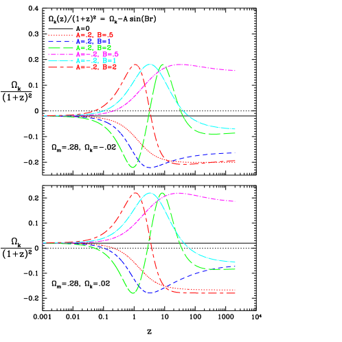
Figure 1: Oscillating curvature models with $B=0.5$, 1, and 2.

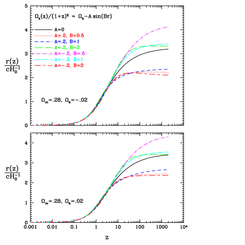
Figure 2: The coordinate distance $r(z)$ for oscillating curvature models in Fig.1, with the same line types.

The age of the universe is given by

$$t(a)=H_{0}^{-1}\int_{0}^{a}\frac{da}{a\,E(a)},$$ (7)

once $\Omega_{k}(z)$, which now depends on $z$ through $r(z)$, has been found numerically.

III Observational constraints on oscillating curvature and the energy content

We use current observational data to constrain the oscillating curvature model given by Eq.(6). Following the approach of WangPia07 , we assume the HST prior of $H_{0}=72\pm 8\,$(km/s)Mpc^-1 HST , use 182 SNe Ia (from the HST/GOODS program Riess07 , the first year Supernova Legacy Survey Astier05 , and nearby SN Ia surveys) Riess07 , CMB data Spergel06 , and the SDSS measurement of the baryon acoustic oscillation scale Eisen05 . We use the CMB data in the form of the CMB shift parameters $R\equiv\sqrt{\Omega_{m}H_{0}^{2}}\,r(z_{CMB})$ and $l_{a}\equiv\pi r(z_{CMB})/r_{s}(z_{CMB})$ derived from WMAP three year data by WangPia07 .

We run a Markov Chain Monte Carlo (MCMC) Lewis02 to obtain ${\cal O}$($10^{6}$) samples for each set of results presented in this paper. The chains are subsequently appropriately thinned.

Due to the degeneracies between $A$, $B$, and $\Omega_{k}$, ($A$, $B$, $\Omega_{k}$) are not well constrained when they are all allowed to vary. To illustrate the effect of oscillating curvature, let us study the class of models given by Eq.(6) for fixed representative values of $B$, while allowing $A$ and $\Omega_{k}$ to vary, along with $\Omega_{m}$, $\Omega_{b}h^{2}$, and $h$ (see WangPia07 ). The parameters estimated from data are ($\Omega_{m}$, $\Omega_{b}h^{2}$, $h$, $\Omega_{k}$, $A$). It should be noted that $A$ affects the overall amplitude of the curvature term, while $B$ plays the role of its oscillating frequency. The case $B=1$ would correspond to $\Omega_{k}$ oscillating every Hubble time.

Figs.3-6 show the joint confidence contours in the plane ($\Omega_{m}$, $\Omega_{k}$) and ($\Omega_{k}$, $A$) for $B=0.5$, 1, 2, and 5 respectively. The inner and outer contours correspond to 68% and 95% confidence levels respectively.

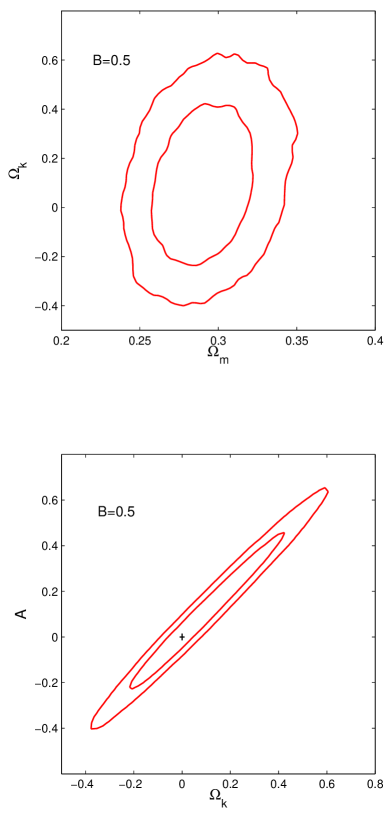
Figure 3: Joint confidence contour plots for ($\Omega_{m}$, $\Omega_{k}$) and ($\Omega_{k}$, $A$) for $B=0.5$. The inner and outer contours correspond to 68% and 95% confidence levels respectively.

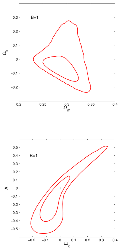
Figure 4: Joint confidence contour plots for ($\Omega_{m}$, $\Omega_{k}$) and ($\Omega_{k}$, $A$) for $B=1$. The inner and outer contours correspond to 68% and 95% confidence levels respectively.

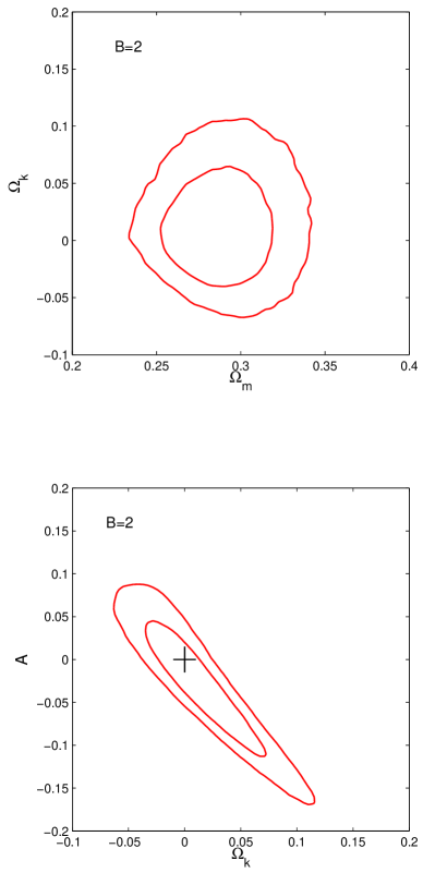
Figure 5: Joint confidence contour plots for ($\Omega_{m}$, $\Omega_{k}$) and ($\Omega_{k}$, $A$) for $B=2$. The inner and outer contours correspond to 68% and 95% confidence levels respectively.

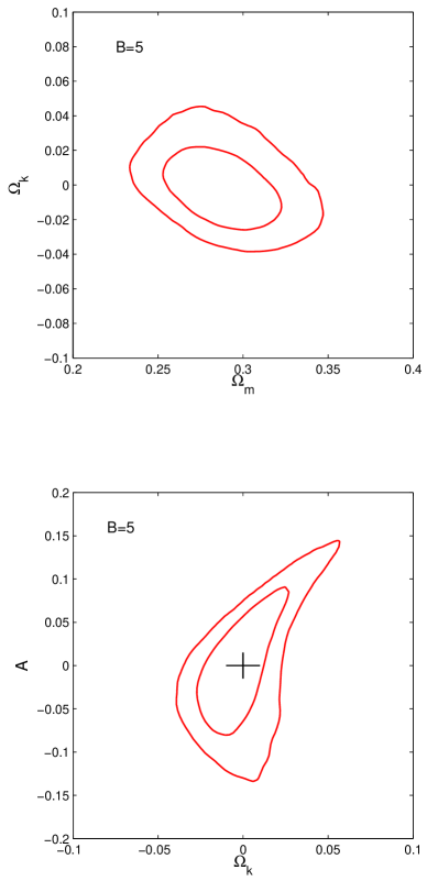
Figure 6: Joint confidence contour plots for ($\Omega_{m}$, $\Omega_{k}$) and ($\Omega_{k}$, $A$) for $B=5$. The inner and outer contours correspond to 68% and 95% confidence levels respectively.

As can be seen from the plots given in Figs.3-6, current data allow models in which the curvature of the universe oscillates with cosmic time. The allowed range of the current curvature density ratio $\Omega_{k}$ is significantly increased compared to the case of constant curvature.

The bounds derived from the WMAP three year data and galaxy survey data from the SDSS sdss give for the case of constant curvature, $\Omega_{k}=-0.005\pm 0.006$, (2dF data 2df also give similar results) Spergel06 . Comparing these bounds to the case of oscillating curvature models, we find that the constraints on the geometry of the universe change significantly, now we have $\Omega_{k}=0.097\pm 0.210$ for $B=0.5$, $\Omega_{k}=-0.037\pm 0.092$ for $B=1$, $\Omega_{k}=0.014\pm 0.035$ for $B=2$, and $\Omega_{k}=0.000\pm 0.017$ for $B=5$. The constraints on the $\Omega_{k}$ and $A$ become more stringent as $B$ increases. This is as expected, since $B$ is the curvature oscillation frequency. For large $B$, the cumulative effect of the oscillating curvature decreases. It is very interesting that when the period of the curvature oscillation $B^{-1}$ becomes larger than a Hubble time, the range of the allowed values for $\Omega_{k}$ and $\Omega_{m}$, at $95\%$ confidence level in agreement with data, shows a drastic increase. An oscillation in the curvature with a period larger than the age of the universe, a case which locally would appear as nearly a constant while being globally notrivial, the time dependence of which would otherwise not be captured by data, does in fact contain a significant deviation from the priors of a simple $LCDM$ model with constant or zero curvature. This is one of our important results: a highly nontrivial geometry on scales larger than the horizon can lead to a very different interpretation of data.

Let us now investigate the implications of the oscillating curvature for the dark energy equation of state $w$. This is done by conducting a likelihood analysis using MCMC of the oscillating curvature model, Eq.(6), assuming a constant dark energy equation of state $w_{X}(z)=w$. The parameters estimated from data are ($\Omega_{m}$, $\Omega_{b}h^{2}$, $h$, $\Omega_{k}$, $A$, $w$). Fig.7 shows the joint confidence contours of ($\Omega_{m}$, $\Omega_{k}$) and ($\Omega_{k}$, $A$), and Fig.8 shows the joint confidence contour of ($\Omega_{k}$, $w$), for $B=5$. As expected, adding $w$ as an additional parameter to be estimated from data notably increase the uncertainties on estimated parameters, especially ($\Omega_{k}$, $A$, $w$). For example, for $B=5$, $\Omega_{k}=0.074\pm 0.068$ when $w$ is included as an estimated parameter, compared with $\Omega_{k}=0.000\pm 0.017$ for setting $w=-1$ (a cosmological constant). For larger values of the period $B^{-1}$, the uncertainties on ($\Omega_{k}$, $A$, $w$) increase significantly. Notice that the bounds on $w$, as shown in Fig.8 for the case $B=5$ can be as large as $-1.04\leq w\leq-0.71$ at $95\%$ confidence level. These bounds on $w$ should be contrasted to the constraints derived in melchiorri where a prior of $\Omega_{k}=0$ was assumed. Clearly, current precision cosmology data is not sufficient in pinning down the equation of state for dark energy when the geometry of the universe is nontrivial.

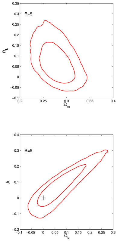
Figure 7: Joint confidence contour plots for ($\Omega_{m}$, $\Omega_{k}$) and ($\Omega_{k}$, $A$) for $B=5$. The inner and outer contours correspond to 68% and 95% confidence levels respectively.

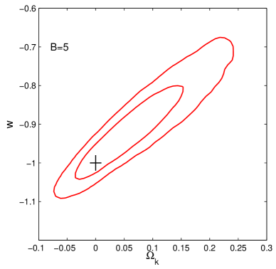
Figure 8: Joint confidence contour plots for ($\Omega_{k}$, $w$) for $B=5$. The inner and outer contours correspond to 68% and 95% confidence levels respectively.

IV Discussion

We have studied constraints on the parameters of a landscape motivated cosmological model in which the curvature of the universe oscillates with cosmic time (see Eq.(6)). Such a model is motivated from the proposal for a dynamic selection of the initial conditions for our universe from the landscape phase space. Thus an analysis of the kind performed here could lead to the implicit detection of quantum gravity effects.

We have used CMB data in the form of the shift parameters $R$ and $l_{a}$ extracted from WMAP three year data by WangPia07 , together with the SDSS measurement of baryon acoustic oscillation scale Eisen05 , and SN Ia data from HST and ground-based observations Riess07 ; Astier05 . From the bounds derived on the parameters of this model we find that currently a simple flat model, which is a special case of the above model, remains a good bet; such a conclusion will be supported further by model selection arguments Pia06 . Allowing for nontrivial geometry leads to greater uncertainties in our knowledge of the present day curvature and matter density ratios $\Omega_{k}$ and $\Omega_{m}$, as can be seen in Figs.3-8). An oscillating curvature term also significantly changes the bounds on the dark energy equation of state $w$, as seen in Fig.8.

It would be interesting to look for the imprints of such a model as data get better. Future dark energy experiments from both ground and space Wang00a ; detf ; ground ; jedi , together with CMB data from Planck planck , should dramatically improve our ability to constrain cosmic curvature, and probe possible imprints of quantum gravity.

Acknowledgements L.M.H is supported in part by DOE grant DE-FG02-06ER41418 and NSF grant PHY-0553312. Y.W is supported in part by NSF CAREER grant AST-0094335 (YW). PM is supported by PPARC, UK.

References

- (1) C.L.Bennett et al., “First Year Wilkinson Microwave Anisotropy Probe (WMAP) Observations: Preliminary Maps and Basic Results,” Astrophys. J. Suppl. 148, 1 (2003),[arXiv:astro-ph/0302207]
- (2) Tegmark, M., et al. 2004, ApJ, 606, 702
- (3) Percival, W., et al., MNRAS, 327, 1297 (2001); Verde, L., et al., 2002, MNRAS, 335, 432; Hawkins, E., et al. 2003, MNRAS, 346, 78
- (4) Riess, A.G., et al., astro-ph/0611572; A. G. Riess et al. [Supernova Search Team Collaboration], Astron. J. 116, 1009 (1998) [arXiv:astro-ph/9805201]
- (5) S. Perlmutter et al. [Supernova Cosmology Project Collaboration], Astrophys. J. 517, 565 (1999) [arXiv:astro-ph/9812133]
- (6) D.N. Spergel, et al. 2006, astro-ph/0603449, ApJ, in press
- (7) M. Tegmark, et al., Phys.Rev. D74 (2006) 123507
- (8) R. Holman and L. Mersini-Houghton, arXiv/hep-th 0511102, in press, Phys. Rev. D (2006).
- (9) R. Holman and L. Mersini-Houghton, arXiv/hep-th 0512070, submitted to Class. Quantum Gravity (2006); L. Mersini-Houghton, “Einstein’s Jury: The Race to Test Relativity”, Princeton. Univ.. Press, [arXiv:hep-th/0512304], [arXiv:hep-ph/0609157].
- (10) L. Mersini- Houghton, [arXiv: gr-qc/0609006]
- (11) C. Kiefer, Clas. Quant. Grav. 4 (1987) 1369; J. J. Halliwell and S. W. Hawking, Phys. Rev. D. bf 31 (1985) 8
- (12) R. Holman, L. Mersini-Houghton and T. Takahashi, arXiv:hep-th/0611223,(2006);R. Holman, L. Mersini-Houghton and T. Takahashi, arXiv:hep-th/0612142, (2006)
- (13) Y. Wang and P. Mukherjee, [arXiv:astro-ph/0703780]
- (14) W. L. Freedman, et al. 2001, ApJ, 553, 47
- (15) A.G. Riess, et al., astro-ph/0611572
- (16) Astier, P., et al. 2005, astro-ph/0510447, Astron. Astrophys. 447 (2006) 31
- (17) D. Eisenstein, et al., ApJ, 633, 560
- (18) A. Lewis and S. Bridle, 2002, PRD, 66, 103511
- (19) Melchiorri,A.,Mersini,L.,Odman,C.,Trodden,M. (2003), Phys.Rev.D68,43509, [arXiv:astro-ph/0211522]
- (20) Planck Bluebook, http://www.rssd.esa.int/index.php?project=PLANCK
- (21) Wang, Y. 2000, ApJ 531, 676
- (22) Albrecht, A.; Bernstein, G.; Cahn, R.; Freedman, W. L.; Hewitt, J.; Hu, W.; Huth, J.; Kamionkowski, M.; Kolb, E.W.; Knox, L.; Mather, J.C.; Staggs, S.; Suntzeff, N.B., Report of the Dark Energy Task Force, astro-ph/0609591
- (23) See for example, http://www.astro.ubc.ca/LMT/alpaca/; http://www.lsst.org/; http://www.as.utexas.edu/hetdex/. detf contains a more complete list of future dark energy experiments.
- (24) Wang, Y., et al., BAAS, v36, n5, 1560 (2004); Crotts, A., et al. (2005), astro-ph/0507043; Cheng, E.; Wang, Y.; et al., Proc. of SPIE, Vol. 6265, 626529 (2006); http://jedi.nhn.ou.edu/
- (25) P. Mukherjee, D. Parkinson and A.R. Liddle, ApJ, 638, 51 (2006); D. Parkinson, P. Mukherjee and A.R. Liddle, Phys.Rev. D73 (2006) 123523