The shapes of molecular cloud cores in Orion

Abstract

We investigate the intrinsic shapes of starless cores in the Orion GMC, using the prestellar core sample of Nutter & Ward-Thompson (2007), which is based on submillimeter SCUBA data. We employ a maximum-likelihood method to reconstruct the intrinsic distribution of ellipsoid axial ratios from observations of the axial ratios of projected plane-of-the-sky core ellipses. We find that, independently of the details of the assumed functional form of the distribution, there is a strong preference for oblate cores of finite thickness. Cores with varying finite degrees of triaxiality are a better fit than purely axisymmetric cores although cores close to axisymmetry are not excluded by the data. The incidence of prolate starless cores in Orion is found to be very infrequent. We also test the consistency of the observed data with a uniform distribution of intrinsic shapes, where oblate and prolate cores of all degrees of triaxiality occur with equal probability. Such a distribution is excluded at the $0.1\%$ level. These findings have important implications for theories of core formation within molecular clouds.

1 Introduction

The intrinsic shapes of molecular cloud cores encode important clues about the processes of molecular cloud fragmentation and core formation. If cores form as the result of converging turbulent flows (e.g., see review by MacLow & Klessen 2004) then they are expected to have random, triaxial shapes, with a slight preference for prolateness (Gammie et al. 2003; Li et al. 2004). If, on the other hand, magnetic fields are dynamically important, and ambipolar diffusion mediates the core formation process, then the cores are expected to be flattened along the magnetic field due to the extra magnetic force acting perpendicular to the field lines. Core shapes in this case are oblate (Mouschovias 1976) although not necessarily axisymmetric (Basu & Ciolek 2004; Ciolek & Basu 2006). Unfortunately, the distribution of core shapes cannot be easily derived from observations, because it is not possible to directly deproject the shape of each core - statistical techniques have to be used instead. Early work on core shapes, assuming axial symmetry, seemed to favour prolate cores (Myers et al. 1991; Ryden 1996). However, subsequent investigations which relaxed the axisymmetry assumption have consistently yielded triaxial, preferentially oblate core shapes (e.g. Jones et al. 2001; Jones and Basu 2002; Goodwin et al. 2002), independently of tracer or core sample.

In light of the recent debate concerning the core formation timescale and its use as a test for theories of core formation in molecular clouds (Hartmann et al. 2001; Tassis & Mouschovias 2004; Ballesteros-Paredes & Hartmann 2006; Mouschovias, Tassis & Kunz 2006), the timing is especially opportune to revisit the question of the intrinsic core shapes, as these may serve as an independent test of theories of core formation. The recent progress in studies of turbulence-driven core formation and the convergence of the findings of different groups concerning the expected distribution of core shapes in this scenario (Gammie et al. 2003; Li et al. 2004) also offers an unprecedented opportunity for direct comparison between theory and observations. We approach the problem using a new statistical method: a maximum-likelihood analysis, aimed to reconstruct the intrinsic shape distribution of molecular cloud cores. Maximum-likelihood analyses are particularly powerful because they allow treatment of different functional forms of the intrinsic shape distribution, distinguishing between functional forms, and explicitly account for observational uncertainties and different assumptions about potential biases in viewing angles. Although here we present a first treatment under the simplest possible assumptions, the expansion of the formalism to include more complicated scenarios is straightforward and we will pursue it in a future publication.

We use the recently released core dataset of Nutter & Ward-Thompson (2007) (NWT07), which offers the opportunity to work with a sample with a series of unique features: a high level of completeness (NWT07 use this sample to derive the core mass function in the mass range $0.3$ to $\sim 100{\rm M_{\odot}}$); cores of varying sizes and masses identified in a single survey [in this case, a SCUBA (Submillimeter Common User Bolometer Array) survey of the Orion Giant Molecular Cloud (GMC)]; confident discrimination between prestellar and protostellar cores (protostellar cores were identified by the authors using Spitzer data, and we have excluded such cores from our analysis). The sample used here consists of the 286 prestellar cores from the Orion A North and South and Orion B North and South star forming regions. Axial ratios for these objects are calculated from the quoted semi-major and semi-minor dimensions in NWT07.

2 Formalism

Consider a system of coordinates centered on a triaxial ellipsoid model molecular cloud core with principal axes ($a$, $b$, $c$). The triaxial ellipsoid surface in this system obeys

$$\frac{x^{2}}{a^{2}}+\frac{y^{2}}{b^{2}}+\frac{z^{2}}{c^{2}}=1\,.$$ (1)

The image of the core appears on the plane of the sky as an ellipse, the properties of which can be calculated from Eq. (1) and the orientation of the observer’s line of sight (Binney 1985). If $a\geq b\geq c$ and we define the axial ratios $\zeta\equiv b/a$ and $\xi\equiv c/a$, so $1\geq\zeta\geq\xi$, the plane-of-the-sky isophotes of the core will be coaxial ellipses of axial ratio

$$q(\theta,\phi,\zeta,\xi)=\sqrt{\frac{A+C-\sqrt{(A-C)^{2}+B^{2}}}{A+C+\sqrt{(A-C)^{2}+B^{2}}}}\,\leq 1$$ (2)

where $\theta$ and $\phi$ are the line-of-sight orientation angles and

$$A\equiv\frac{\cos^{2}\theta}{\xi^{2}}\left(\sin^{2}\phi+\frac{\cos^{2}\phi}{\zeta^{2}}\right)+\frac{\sin^{2}\theta}{\zeta^{2}}\,,$$ (3)

$$B\equiv\cos\theta\sin 2\phi\left(1-\frac{1}{\zeta^{2}}\right)\frac{1}{\xi^{2}}\,,\,C\equiv\left(\frac{\sin^{2}\phi}{\zeta^{2}}+\cos^{2}\phi\right)\frac{1}{\xi^{2}}\,.$$ (4)

The axial ratio $q$ has values limited between $0$ and $1$. A very elongated ellipse has $q\ll 1$, while a circle has $q=1$.

Let the cores of the Orion GMC have a single intrinsic distribution of shapes, $p_{\rm Orion}(\zeta,\xi)d\zeta d\xi$, defined as the fraction of cores with axial ratios between $\zeta$ and $\zeta+d\zeta$ and $\xi$ and $\xi+d\xi$. Let us assume that $p_{\rm Orion}$ can be parametrized by a set of parameters $C_{i}$. From an assumed $p_{\rm Orion}(\zeta,\xi,C_{i})$, we can calculate the distribution of axial ratios of projected cloud ellipses, $p(q)$, by assuming that the viewing angles are random ($\phi$ and $\cos\theta$ follow uniform distributions). For this calculation we use the following Monte-Carlo method:

(i) We select a set of parameters $C_{i}$ for the distribution $p_{\rm Orion}(\zeta,\xi,C_{i})$.

(ii)We randomly draw a pair of ($\zeta,\xi$) from the distribution $p_{\rm Orion}(\zeta,\xi,C_{i})$, and a pair of ($\theta$, $\phi$) from a uniform probability distribution (equal probability for any value of $\cos\theta$ or $\phi$ in the intervals $[-1,1]$ and $[0,2\pi]$ respectively). We use the values of $\zeta,\xi,\theta,\phi$ to calculate $q$ through Eq. (2)

(iii) We repeat steps (i)-(ii) a large number of times. We bin the obtained values of $q$, and we normalize the obtained distribution $p(q)$ so that it is a probability density function (pdf) ($\int_{1}^{\infty}p(q,C_{i})dq=1$).

Once we have obtained $p(q,C_{i})$, we can calculate the likelihood function $\mathcal{L}$. If we have $n$ observations of core axial ratios $q_{1},q_{2},...q_{n}$ then, dropping constant normalization factors, the likelihood is

$$\mathcal{L}(C_{i},q_{1},q_{2},....,q_{n})=\prod_{j=1}^{n}p(q_{j},C_{i})$$ (5)

The maximum-likelihood parameters of the intrinsic shape distribution $p(\zeta,\xi,C_{i})$ are that set of $C_{i}$ which maximize the likelihood $\mathcal{L}$ for our given set of observed axial ratios.

Performing a likelihood analysis requires a selection of a functional form for the intrinsic shape distribution $p(\zeta,\xi)$. Lacking any a priori knowledge on the functional form of $p(\zeta,\xi)$, we have chosen functional forms based on their simplicity and appropriateness of their properties (defined in finite domains, singly-peaked). We will perform this analysis using two distinct families of distributions to test the sensitivity of our result to the assumed functional form. In the following sections, we briefly discuss these functional forms.

2.1 Beta Distribution of Axial Ratios

Since both $\zeta$ and $\xi$ are defined in finite domains, a natural choice is the beta distribution, which is routinely used to model events which are constrained within finite value intervals. The probability density function of the beta family of distributions is $p(x)=x^{a-1}(1-x)^{b-1}/B(a,b)$, where $B(a,b)=\int_{0}^{1}t^{a-1}(1-t)^{b-1}dt$ is the beta function. The distribution is defined in the interval [0,1] and its shape is controlled by the non-negative shape parameters $a,b$. When $a,b>1$ the distribution is singly-peaked.

We construct a joint distribution $p(\zeta,\xi)$ assuming that $\zeta$ follows a beta distribution with domain $(0,1]$ and $\xi$ follows a beta distribution with domain $(0,\zeta]$. We start from a double beta distribution in variables $x$ and $y$, which vary between $0$ and $1$, with shape parameters ($a_{x},b_{x}$) and ($a_{y},b_{y}$), respectively. With the change of variables $\zeta=x$ and $\xi=\zeta y$ [which maps the $(0,1]$ domain of $y$ to the desired $(0,\zeta]$ domain of $\xi$], we obtain the joint distribution for $\zeta,\xi$:

$$p(\zeta,\xi) = \frac{\zeta^{a_{x}-a_{y}-b_{y}}(1-\zeta)^{b_{x}-1}\xi^{a_{y}-1}(\zeta-\xi)^{b_{y}-1}}{B(a_{x},b_{x})B(a_{y},b_{y})}\,.$$ (6)

The joint probability of Eq. (6) is such that $\zeta$ and $\xi$ are not independent. The distribution of Eq. (6) has a single peak at

$$\xi_{0}=\frac{a_{y}-1}{a_{y}+b_{y}-2}\zeta_{0}\,,\,\,\,\,\,\,\,\,\,\,\zeta_{0}=\frac{C_{1}C_{2}-b_{y}+1}{C_{1}C_{3}-b_{y}+1}$$ (7)

provided that $a_{y},b_{y}>1$ and that $a_{x},b_{y}$ are such that $0<\zeta_{0}<1$. In Eq. (7) $C_{1}=(1-b_{y})/(a_{y}+b_{y}-2)$, $C_{2}=a_{x}-a_{y}-b_{y}$, and $C_{3}=a_{x}-a_{y}+b_{x}-b_{y}-1$. In our analysis, we only admit values of the shape parameters that result in a singly-peaked distribution. This is a tetra-parametric distribution and the likelihood analysis is aimed at determining the values of $a_{x}$, $b_{x}$, $a_{y}$, and $b_{y}$.

2.2 Modified Lognormal

We construct this distribution by seeking an appropriate minimal transformation which transforms the domain of $\zeta$ and $\xi$ from $(0,1)$ to $(-\infty,\infty)$; we then take the transformed variables to follow a Gaussian distribution. Such an appropriate transformation is $\zeta\rightarrow x$ and $\xi\rightarrow y$ where $x=\ln[\zeta/(1-\zeta)]$ and $y=\ln[\xi/(\zeta-\xi)]$. Assuming a double Gaussian pdf of $x$ and $y$, the joint pdf of $\zeta$ and $\xi$ is

$$p(\zeta,\xi) = \frac{\exp\left[-\frac{(\ln\frac{\zeta}{1-\zeta}-x_{0})^{2}}{2\sigma_{x}^{2}}\right]\exp\left[-\frac{(\ln\frac{\zeta}{1-\zeta}-x_{0})^{2}}{2\sigma_{x}^{2}}\right]}{2\pi\sigma_{x}\sigma_{y}\xi(\zeta-\xi)(1-\zeta)}$$ (8)

This is also a tetra-parametric distribution and the likelihood analysis is aimed at determining the values of $x_{0}$, $y_{0}$, $\sigma_{x}$, and $\sigma_{y}$. Due to the transformation used to project the $(0,1)$ interval to $(-\infty,\infty)$, the distribution in ($\zeta,\xi$) space is skewed with respect to the original Gaussian shape of the distribution in ($x,y$) space. The distortion increases as $\sigma_{x}$ and $\sigma_{y}$ increase, and eventually the distribution acquires additional local maxima. To avoid such extreme distortions we limit the range of $\sigma_{x}$ and $\sigma_{y}$ by imposing a prior requirement in our likelihood analysis that $\sigma_{x},\sigma_{y}\leq 0.7$.

3 Results

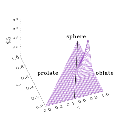
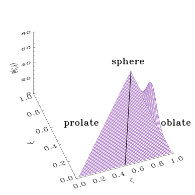
Figure 1: Upper panel: maximum-likelihood modified beta-distribution; lower panel: maximum-likelihood modified lognormal distribution

Figure 2: Contours of the likelihood function at a level of $\sim 1/3$, $\sim 1/22$ and $\sim 1/100$ smaller than the value at the maximum. Upper panel: $a_{y},b_{y}$ are fixed at their maximum-likelihood values; lower panel: $a_{x},b_{x}$ are fixed at their maximum-likelihood values.

Figure 3: Distribution of axial ratios (minor/major axis) of projected starless core ellipses (datapoints). The lines show the projected core ellipse distributions derived from a uniform intrinsic shape distribution (solid line), the maximum-likelihood beta-distribution (dotted line) and the maximum-likelihood lognormal (dashed line).

The upper panel of Fig. 1 shows surface plots of the maximum-likelihood distribution for the beta-family of distributions. Its shape parameters were obtained by maximizing the likelihood function, using the “Simulated Annealing” algorithm (Corana et al. 1987). On the $\zeta-\xi$ plane we have indicated the dividing line between oblate and prolate cores (oblate cores have $\zeta>0.5(1+\xi)$). On this plane, spheres live at $\zeta=\xi=1$, infinitesimally thin axisymmetric disks have ($\zeta=1$, $\xi=0$) and infinitesimally thin cigars have ($\zeta=0$, $\xi=0$). Finite-thickness axisymmetric disks live along the $\zeta=1$ line. The most likely distribution of intrinsic shapes is peaked at $\zeta\approx 1$ and $\xi\approx 0.54$, indicating that the most probable shape is a finite-thickness disk with small deviations from axisymmetry. However, larger degrees of triaxiality are also frequently encountered, as the distribution decreases only gradually with decreasing $\zeta$. Even so, only a very small fraction of objects in this distribution are prolate. The distribution peaks strongly at oblate shapes.

To test the sensitivity of our likelihood analysis to the assumed functional form of the intrinsic shape distribution, in the lower panel of Fig. 1 we plot the maximum-likelihood modified lognormal distribution. Although the detailed shape of the two maximum-likelihood distributions is different, their overall features are in remarkable agreement. The distributions are strongly peaked at about the same point ($\zeta\sim 1$, $\xi\sim 0.5$), indicating that the most probable intrinsic shape of cores found in the Orion star-forming regions is predominantly oblate, and the half-thickness of the cores is finite (about one-quarter the diameter of the disk).

Qualitatively this result is to be expected, as most of the elongation measurements indicate projected ellipses with low elongations, while there are also a few cores with significant elongations. If viewed from various random angles, an oblate core will most of the time yield an only mildly elongated projection (face-on or almost face-on observations), while in the few cases when the core is viewed edge-on or close to edge-on, a significantly elongated projection will result. In contrast, a prolate core viewed at random angles will most of the time yield a significantly elongated projection, a result not corroborated by the data (see Fig. 3 and discussion below).

Figure 2 gives a sense of the uncertainty associated with our determination of the intrinsic shape distribution parameters. It shows contours of the likelihood function for the beta-family of distributions. In the upper panel, we plot contours of the likelihood as a function of $1/a_{x}$ and $1/b_{x}$, with $a_{y}$ and $b_{y}$ fixed at their maximum-likelihood values. The ($a_{x}$, $b_{x}$) parameters primarily control the shape of the distribution along the $\zeta$ axis. The straight line represents the division between the regime where the peak of $p(\zeta,\xi)$ corresponds to an oblate object (lower right), and the regime where the peak corresponds to a prolate object (upper left), assuming that the other two parameters ($a_{y},b_{y}$) are fixed at their maximum-likelihood values. The contours correspond to a reduction of the level of the likelihood with respect to its maximum value of $\sim 1/3$, $\sim 1/22$ and $\sim 1/100$, which would be the levels of the $1,2$ and $3\sigma$ contours for a 2-parameter likelihood with $\log\mathcal{L}$ falling as a chi-square distribution. The likelihood is very strongly peaked at the oblate part of the plane, with the likelihood of a prolate peak being infinitesimal.

The lower panel shows the same-level contours for the likelihood as a function of $1/a_{y}$ and $1/b_{y}$, with $a_{x}$ and $b_{x}$ fixed at their maximum-likelihood values. The $a_{y}$, $b_{y}$ parameters primarily control the shape of the distribution along the $\xi$ axis. In this case, there is no dividing line since the distribution peak would correspond to an oblate object for any pair of ($a_{y}$, $b_{y}$) for the given values of $a_{x},b_{x}$: the latter fix the peak along the $\zeta$ axis very close to $\zeta=1$, and objects with such high $\zeta$ are always oblate independently of the value of $\xi$. The likelihood is concentrated close to the diagonal, and has a preference for comparable values for $a_{y}$ and $b_{y}$, indicating that, along the $\xi$-axis, the intrinsic shape distribution is roughly symmetric. The slight ringing at the lower-left corner of the plot is a numerical effect due to the finite resolution in our calculation of the likelihood, and does not affect the values of our maximum-likelihood parameters since it occurs sufficiently far from the likelihood maximum.

Figure 3 shows the distribution of axial ratios for the projected core ellipses derived from three intrinsic shape distributions: the maximum-likelihood beta-distribution (dotted line), the maximum-likelihood lognormal distribution (dashed line), and a uniform distribution, $p_{\rm Orion}(\zeta,\xi)=$const. (solid line). The crosses correspond to the NWT07 data, binned in intervals of $\Delta q=0.05$. The uniform intrinsic shape distribution roughly approximates a distribution of core shapes expected from turbulence-driven cloud fragmentation and core formation (e.g. Gammie et al. 2003; Li et al. 2004). That the maximum-likelihood distributions are a better fit to the data is immediately obvious. We have also performed a Kolmogorov-Smirnov test to quantify the discrepancy between the data and the uniform distribution, and to verify that the maximum-likelihood distributions are in fact likely in absolute terms to reproduce the observed dataset. We find that the probability that the observed data come from the uniform intrinsic shape distribution is smaller than $0.1\%$. The same test indicates that the dataset is consistent within the $1\sigma$ level with originating from either of the maximum-likelihood distributions, which are peaked at oblate intrinsic shapes.

A potential source of bias in this analysis is the resolution limitations of the data. It is conceivable that, for smaller-sized cores, the actual semi-major and semi-minor axes of the projected core ellipse are both comparable to, or smaller than, the smallest angle that can be resolved in the data. Such a case would lead to an observational bias toward circular core ellipses for the smallest objects, in which case our statistical analysis would lead to erroneous results. We have checked that this is not the case in our dataset. The largest number of our smallest elongation cores were not, in fact, close to the resolution limit. In addition, as we can see in Fig. 3, there is no “pileup” of cores towards $q=1$, as would be expected if the bias discussed here were significant.

4 Discussion

We have derived the maximum-likelihood beta-distribution of intrinsic shapes for the Orion GMC starless molecular cloud cores of the NWT07 set. The maximum-likelihood distribution peaks at the shape of an oblate, finite-thickness, nearly axisymmetric disk. Oblate cores of varying thickness and varying degrees of triaxiality also occur frequently, however the distribution falls very quickly to zero in the prolate part of the spectrum of shapes. Cores in Orion are most likely intrinsically oblate. This main result is robust with respect to differences in the assumed functional form of the intrinsic distribution. Our result is consistent with the findings of Jones et al. (2001) and Jones & Basu (2002), who used different datasets and a different statistical treatment. Hence, it appears that the result that molecular cloud cores are preferentially oblate is also robust to the details of the dataset used, the wavelength of the observations, and the details of the statistical treatment. A uniform distribution of shapes with equal numbers of oblate and prolate cores is rejected by the data at a high confidence level ($<0.1\%$).

These results are particularly interesting since they can have important implications for theories of core formation. Turbulence-induced core formation tends to favor uniform triaxial shape distributions with, if anything, a slight preference for prolate starless cores (e.g. Gammie et al. 2003; Li et al. 2004). Such distributions are not preferred by the observational data. In contrast, magnetically-driven fragmentation naturally leads to oblate objects due to the extra magnetic support perpendicular to the field lines.

An additional effect beyond the core formation process which could, in principle, alter the shape of molecular cloud cores and introduce a bias favoring oblate shapes is rotation. However, the ratios of rotational and gravitational energy in prestellar cores such as the ones examined here are observed to be very small (typically $<$ few percent) and there are no observational indications of rotational flattening (e.g. Goodman et al. 1993; Caselli et al. 2002). Even these small amounts of angular momentum can lead to appreciable flattening and rotationally supported discs after sufficient contraction under angular momentum conservation - however, such flattening becomes important in much later contraction stages, and at small ($<10^{3}{\rm\,AU}$) scales (overall, protostellar core shapes are not significantly different than those of prestellar cores, e.g. Goodwin et al. 2002). Similar results on the absence of rotationally-induced flattening are also found in simulations (Gammie et al 2003; Li et al. 2004).

The maximum-likelihood approach used in this work is a powerful statistical technique, which can be appropriately expanded to explicitly account for observational uncertainties and be combined with magnetic field orientations from polarization data as those become available.

Other than observational uncertainties, our results may be biased by three additional factors. First, in order to derive shapes from the signal-to-noise submillimeter maps, one makes the implicit assumption of core isothermality, so that emissivity contours truly correspond to the spatial distribution of core mass. This source of uncertainty is not of great concern, however, because on the one hand isothermality is likely to be an excellent approximation for starless cores especially at the outer edges of the core defining its shape. On the other hand, deviations from isothermality would only affect the shape determination if the temperature gradient does not follow the density gradient, which is not expected for gravitational heating. A second potential complication is that these cores all originate in the same GMC. If there is a preferential direction in this cloud set by the large-scale magnetic field and if the magnetic field is dynamically important, then cores may be preferentially oriented with their smallest ellipsoid axes aligned with the magnetic field, which might weaken our assumption of random viewing angle orientations. However, in the turbulent core formation scenario, this is not a concern since the magnetic field is in this case dynamically unimportant and tangled. Therefore, the comparison of the observed core distribution at least with the predictions of the turbulence theory of core formation is not affected by such a bias, and this effect cannot ameliorate the discrepancy between roughly uniform shape distributions and the observed data. Additionally, the survey area from which our dataset was derived spans a $10^{\circ}$ region in the sky, rather than a single small cloud where orientation biases would be expected to be most significant. Finally, it is conceivable that the intrinsic shape distribution is not singly-peaked, but involves two distinct peaks in different regions of the $(\zeta,\xi)$ parameter space.

References

- [Basu & Ciolek(2004)] Basu, S., & Ciolek, G. E. 2004, ApJ, 607, L39
- [Binney(1985)] Binney, J. 1985, MNRAS, 212, 767
- [Caselli et al.(2002)] Caselli, P., Benson, P. J., Myers, P. C., Tafalla, M. 2002, ApJ, 572, 238
- [Ciolek & Basu(2006)] Ciolek, G. E., & Basu, S. 2006, ApJ, 652, 442
- [Corana et al.(1987)] Corana, A., Marchesi, M., Martini, C., Ridella, S. 1987, ACM Trans. Math. Soft., 13, 262
- [Gammie et al.(2003)] Gammie, C. F., Lin, Y.-T., Stone, J. M., Ostriker, E. C. 2003, ApJ, 592, 203
- [Goodman et al.(1993)] Goodman, A. A., Benson, P. J., Fuller, G. A., Myers, P. C. 1993, ApJ, 406, 528
- [Goodwin et al.(2002)] Goodwin, S. P., Ward-Thompson, D., Whitworth, A. P. 2002, MNRAS, 330, 769
- [Jones et al.(2001)] Jones, C. E., Basu, S., Dubinski, J. 2001, ApJ, 551, 387
- [Jones & Basu(2002)] Jones, C. E., Basu, S. 2002, ApJ, 569, 280
- [Kerton et al.(2003)] Kerton, C. R., Brunt, C. M., Jones, C. E., Basu, S. 2003, A&A, 411, 149
- [Li et al.(2004)] Li, P. S., Norman, M. L., Mac Low, M.-M., Heitsch, F. 2004, ApJ, 605, 800
- [Mac Low & Klessen(2004)] Mac Low, M.-M., & Klessen, R. S. 2004, Reviews of Modern Physics, 76, 125
- [Mouschovias(1976)] Mouschovias, T. Ch. 1976, ApJ, 207, 141
- [Myers et al.(1991)] Myers, P. C., Fuller, G. A., Goodman, A. A., Benson, P. J. 1991, ApJ, 376, 561
- [Nutter & Ward-Thompson(2007)] Nutter, D., Ward-Thompson, D. 2007, MNRAS, 374, 1413
- [Ryden(1996)] Ryden, B. S. 1996, ApJ, 471, 822